Abstract
To address a key issue in functional time series analysis on testing the randomness of an observed series, we propose an IID test for functional time series by generalizing the Brock–Dechert–Scheinkman (BDS) test, which is commonly used for testing nonlinear independence. Similarly to the BDS test, the proposed functional BDS test can be used to evaluate the suitability of prediction models as a model specification test and to detect nonlinear structures as a nonlinearity test. We establish asymptotic results for the test statistic of the proposed test in a generic separate Hilbert space and show that it enjoys the same asymptotic properties as those for the univariate case. To address the practical issue of selecting hyperparameters, we provide the recommended range of the hyperparameters. Using empirical data on the VIX index, empirical studies are conducted that feature the applications of the proposed test to evaluate the adequacy of the fAR and fGARCH models in fitting the daily curves of cumulative intraday returns (CIDR) of the index. The results reveal that the proposed test remedies some shortcomings of the existing independence test. Specifically, the proposed test can detect nonlinear temporal structures, while the existing test can only detect linear structures.
1. Introduction
Functional time series analysis combines functional data analysis with time series analysis. Similarly to univariate and multivariate time series, a temporal dependence structure exists in functional observations, which manifest themselves in a graphical form of curves, images, or shapes. Typically, functional time series can be classified into two main categories. Specifically, the first one segments a univariate time series into (sliced) functional time series. For example, Rice et al. (2023) considered intraday volatility to form functional time series defined for a continuum . The other category is when the continuum is not a time variable, such as age (see, e.g., Shang et al. 2022) or wavelength in spectroscopy (see, e.g., Shang et al. 2022).
Over the past two decades or so, there have been rapid developments in functional time series analysis. An important branch of such developments is to extend the mainstream models and analytical tools in univariate time series to functional cases (see, e.g., Kokoszka and Reimherr 2017). To name a few, Kokoszka et al. (2017) and Mestre et al. (2021) proposed a functional autocorrelation function (fACF) to quantify linear serial correlation in a functional time series. Huang and Shang (2023) proposed a nonlinear fACF to measure nonlinear dependence in a functional time series. Bosq (1991) extended the autoregressive (AR) model to the functional case, referred to as the fAR model. Since then, a score of functional time series models have been extended from the fAR model. Some extended models include, for example, the autoregressive Hilbertian with exogenous variables model (ARHX) (Damon and Guillas 2002), the Hilbert moving average model (Turbillon et al. 2007), the functional autoregressive moving average (fARMA) model (Klepsch et al. 2017), the seasonal functional autoregressive model (Zamani et al. 2022), and the seasonal autoregressive moving average Hilbertian with exogenous variables model (SARMAHX) (González et al. 2017). For modeling conditional variance, these extensions include the functional autoregressive conditional heteroskedasticity model (fARCH) (Hörmann et al. 2013), the functional generalized autoregressive conditional heteroskedasticity (fGARCH) model (Aue et al. 2017), and the fGARCH-X model (Rice et al. 2023).
Functional time series analysis has a wide range of applications, including those in financial risk management. For example, Tang and Shi (2021) applied a high-dimensional functional time series method to forecast constituent stocks in the Dow Jones index. Shang (2017) implemented a functional time series approach to forecast intraday S&P 500 index returns. Shang et al. (2019a) considered the problem of dynamic updating for intraday forecasts of the volatility index.
Despite increasing interest and research on functional time series, the existing literature focuses on the use of measures or tools based on autocovariance and/or autocorrelation to investigate the underlying structure of observed functional time series (Horváth et al. 2013; Mestre et al. 2021; Zhang 2016). The independent and identically distributed (IID) test for functional time series is rather limited, with the exception of Gabrys and Kokoszka (2007b), García-Portugués et al. (2019), and Kim et al. (2023). These exceptions only captured the linear temporal structure. Except for nonlinear fACF in Huang and Shang (2023), a relatively little attention has been given to studying the nonlinear temporal structures within the functional time series literature. Additionally, since linear structures restrict these tools, they cannot test all possible deviations from randomness. Therefore, a robust model specification test is required to evaluate the adequacy of functional time series models. In a function-on-function regression, Chiou and Müller (2007) developed a set of diagnostic tools based on residual processes. The latter are defined by subtracting the predicted functions from the observed response functions. This residual process is expanded into functional principal components and their scores. A randomization test is developed based on these scores to examine whether the residual process is related to the covariate, as an indication of lack of fit of the model. However, these diagnostic tools cannot be extended to functional time series due to temporal dependence.
In this paper, we extend the BDS test of Brock et al. (1987) to a functional time series. As in the univariate case, the proposed test can be used as an IID test on estimated residuals to evaluate the adequacy of the fitted model and as a nonlinearity test on residuals of functional time series after removing linear temporal structures exhibited in the investigated data.
The BDS test proposed by Brock et al. (1996) is the most widely used nonlinearity test and model specification test in univariate time series analysis. In empirical studies, the BDS test is often used on financial time series residuals after fitting an ARMA or ARCH-type model to test for the presence of chaos and nonlinearity (Lee et al. 1993; Mammadli 2017; Small and Tse 2003). The reason behind its popularity is mainly twofold:
- (1)
- The BDS test requires minimal assumptions and previous knowledge about the investigated data sets. When the BDS test is applied to model residuals, the asymptotic distribution of its test statistic is independent of estimation errors under certain sufficient conditions (see Chan and Tong 2001, Chapter 5). Specifically, de Lima (1996) showed that for linear additive models or models that can be transformed into that form, the BDS test is nuisance parameter-free and does not require any adjustment when applied to fitted model residuals.
- (2)
- The BDS test tests against various forms of deviation from randomness. While the null hypothesis of the BDS test is that the investigated time series is generated by an IID process, its alternative hypothesis is not specified. It may be thought of as a portmanteau test. This implies that the BDS test can detect any non-randomness exhibited in the investigated time series. Additionally, a fast algorithm exists for computing the BDS test statistics, which ensures the BDS test’s easy and speedy application on empirical applications (LeBaron 1997). Also, the BDS statistic asymptotic distribution theory does not require higher-order moments to exist. This property is especially useful in analyzing financial time series since many financial time series exhibit heavy-tailed distributions whose higher-order moments may not exist.
In the recent literature, Kim et al. (2003) compared the conventional nonparametric tests and the BDS test for residual analysis. They found that the BDS test is more reasonable than the conventional nonparametric tests. Caporale et al. (2005) examined the use of the BDS test when applied to the logarithm of the squared standardized residuals of an estimated GARCH(1,1) model as a test for the suitability of this specification. Extending from Brock et al. (1996), Kočenda (2001) removed the limitation of having to arbitrarily select a proximity parameter by integrating across the correlation integral. Luo et al. (2020) proposed a modified BDS test by removing some terms from the correlation integral, and this addresses the weakness of overly rejecting the null hypothesis in the original BDS test. Escot et al. (2023) recursively applied the BDS test to detect structural changes in financial time series.
The BDS test has its own weaknesses. Luo et al. (2020) contained a revision about some of the known problems of this type of test; among others, the sensitivity with respect to the choice of tuning parameters, low convergence to asymptotic normality, and over-rejection of the null hypothesis.
The rest of this paper is structured as follows. Section 2 provides the specification of the functional BDS test. In Appendix B, we provide detailed proof of the asymptotic distribution of the test statistics of the functional BDS test. In Section 3, we present Monte-Carlo experiments on the IID functional time series and simulated fGARCH(1,1) functional time series to provide the recommended dimension and distance hyperparameters range. In Section 4, the functional BDS test is used to test the adequacy of the fAR(1) and fGARCH models on the fitted residuals of daily curves of intraday VIX index returns. Conclusions are given in Section 5, along with some ideas on how the methodology presented here can be further extended.
2. BDS Test for Functional Time Series
The BDS test uses “correlation integral”, a popular measure in chaotic time series analysis. According to Packard et al. (1980) and Takens (1981), the method of delays can embed a scalar time series into a m-dimensional space as follows:
Accordingly, is called m-history of . Grassberger and Procaccia (1983) proposed correlation integral as a measure of the fractal dimension of deterministic data since it records the frequency with which temporal patterns are repeated. The correlation integral at the embedding dimension m is given by
where N is the size of the data sets, is the number of embedded points in m-dimensional space, r is the distance used for testing the proximity of the data points, and denotes the sup-norm.1
In essence, measures the fraction of the pairs of points , , the sup-norm separation of which is less than r.
Brock (1987) showed that under the null hypothesis are IID with a non-degenerated distribution function ,
According to Brock et al. (1996), the BDS statistic for is defined as
where ,
and . Note that is a consistent estimate of C, and K can be consistently estimated by
Under the IID hypothesis, has a limiting standard normal distribution as .
The above specification of the BDS test is for scalar time series. When the object is a functional time series, one needs to adjust the computation of sup-norm separation of the m-histories in (2) and (9).
Given a functional time series , the m-history of is constructed by its m neighbouring observations, namely
The sup-norm of two sets of m functions can be measured by taking the maximum distance between the corresponding curves. Specifically, if we use norm as the distance measure between two curves,
Since we adjust the specification of the BDS test statistic to be adaptive to the functional case, to determine the critical value of the BDS test after the adjustment, one needs to derive its asymptotic distribution under the null hypothesis. In Appendix B, we prove that the asymptotic normality for the univariate BSD test statistic is also valid for the functional case. Indeed, the asymptotic normality result presented in Theorem 1 of Appendix B is versatile. It holds for any norm on a separable Hilbert space , which is more general than the -norm.
The norm is not the only distance measure of two functions. Other common choices include norm and norm. All of them, including other norms, can be used for computing the sup-norm of m-histories of functional time series. However, the choice for the distance measure determines the recommended range for the distance hyperparameter r as well as the speed of convergence of the test statistic and the power of the test. In Section 3, we present power and size experiments on random and structured functional time series when , and are selected as the distance measure inside the sup-norms.
3. Monte-Carlo Simulation Study
We conduct Monte-Carlo experiments on simulated IID and structured functional time series to provide the recommended range of hyperparameters of the functional BDS test, namely m, r, and the preferred norms inside the sup-norms.
We use three metrics to evaluate the selection of the hyperparameters and the norms: (1) the resemblance of normality of the test statistics on the IID process; (2) the size of the test at 1%, 5% and 10% nominal levels; and (3) the power of rejecting on a structured process. To compare the performance of the functional BDS test with the existing method, the same power experiment is also conducted on the GK independence test proposed by Gabrys and Kokoszka (2007b), a commonly used independence test in the functional time series domain.
For the resemblance of normality, we simulated 200 paths of 500 IID functional time series and computed the BDS test statistic on each path with and , where s.d. denotes the standard deviation of the residual process. Computationally, the standard deviation of the residual process can be computed by the sd.fts function in the ftsa package (Hyndman and Shang 2025). Table 1 provides the p-value of the Kolmogorov–Smirnov (KS) test for each combination of m and r when is selected as the norm inside the sup-norms. Since different types of norm focus on different error loss functions, the respective tables with and being selected as the norms inside the sup-norms are provided in Table A1 in Appendix A.

Table 1.
The p-value of the KS test on functional BDS test statistics with norm computed on 200 paths of 500 simulated IID functional time series. A p-value less than 0.025 is highlighted in bold, indicating the generated BDS test statistics cannot be assumed to follow a standard normal distribution at the 5% significance.
The KS test examines against the null hypothesis that the computed functional BDS test statistic is from a standard normal distribution. A p-value less than 0.025 (highlighted in bold) indicates the rejection of , which means the generated BDS test statistics cannot be assumed to follow a standard normal distribution. On the contrary, the higher the p-value is, the closer the BDS test statistics are to a standard normal distribution.
From the results in Table 1 and Table A1, we can see that the functional BDS test with a moderate m () and a sufficiently large r () ensures that the respective test statistics have distributions sufficiently close to a standard normal distribution under the null hypothesis. The metrics are different ways of quantifying distances. For example, from the perspective of statistical estimation, the -norm corresponds to the least absolute deviation and gives an least-absolute-deviation estimator if it is used as a criterion for estimation, while the -norm corresponds to the least square deviation and gives a least-square estimator if it is used as a criterion for estimation. The -norm corresponds to a maximum deviation and gives rise to a (robust) minimax estimator if it is used as a criterion for estimation. Based on the data sets we used, it is found that the different criteria do not influence the calculation of p-value shown in Table 1 in the main manuscript and Table A1 in Appendix A. However, at an intuitive level, it seems that the -norm may give rise to the most conservative result among the three criteria considered as far as the detection of nonlinear patterns in different types of functional time series is concerned. Indeed, the theoretical results, particularly the asymptotic results, in our paper apply to a general norm on a separable Hilbert space. It is flexible to accommodate different criteria and facilities for the study of the impacts of the choices of different norms on the detection of nonlinearity in different classes of functional time series models.
To examine the size of the test, we compute the probability of falsely rejecting the null hypothesis using the same simulated IID functional time series in the normality resemblance experiments. We conduct the size experiments with a nominal test level at 1%, 5%, and 10% significance levels. Table 2 reports the size of the test with norm at a nominal level of 1% when a different combination of the hyperparameters m and r is selected. The results of the size experiments at the nominal levels of 5% and 10% will be provided in Table A2 in Appendix A. We highlight the cells in bold when the actual sizes of the test exceed the nominal level by 3% or more. The results from the size experiments are consistent with those of the normality resemblance experiments. From Table 2, a moderate m () and a sufficiently large r () ensure an appropriate size of the functional BDS test at the 1% nominal level. However, the results at the nominal levels of 5% and 10% presented in Table A2 appear less conclusive.
Table 2.
The size of the functional BDS test with norm at 1% nominal level computed on 200 paths of 500 simulated IID functional time series. The cells with size of the test exceeding the nominal level by 3% are highlighted in bold.
For the power test, we simulated 200 paths of an fGARCH process proposed by Aue et al. (2017). In each path, we generate 500 observations, and each functional observation is formed by 100 equal-spaced points within (0,1). A sequence of random functions is called a functional GARCH process of order (1,1), abbreviated as fGARCH, if it satisfies the equations
where is a non-negative function, the operators and map non-negative functions to non-negative functions, and the innovations are iid random functions. Our simulated fGARCH processes inherit the format of the simulated fGARCH process in Aue et al. (2017). We set
and the integral operators and to be
where C is a constant. The innovations are defined as
where are IID standard Brownian motions. We specifically choose a small constant in (15), so the generated process has relatively weak temporal structures.
After simulating 200 paths of the fGARCH process, we compute the functional BDS test statistic on each simulated functional time series. Table 3 presents the probability the functional BDS test successfully rejects the IID hypothesis on a structured process when is selected as the norm. Table A3 in Appendix A provides the respective tables with and . A value of 100% indicates that the BDS test made correct inferences at all simulated paths, whereas a value less than 100% suggests it failed to distinguish a structured process from a random one at certain paths. The same statistics of the power experiment on GK test is provided in Table 4. The GK independence test requires two hyperparameters, p and H, since it is based on the lagged cross-covariances of the projected principal components of the functional time series. The hyperparameter p represents the number of retained principal components in the dimension reduction step, and H denotes the maximum lagged cross-covariances considered in computing the test statistics.
Table 3.
The successful rejection rate of the functional BDS test on 200 paths of the simulated fGARCH process of 500 observations with being used as the norm inside the sup-norms and different choices of m and r.
Table 4.
The successful rejection rate of the GK test on 200 paths of the simulated fGARCH process of 500 observations with different choices of H and p.
In Table 3 and Table A3, the results of the power experiments indicate the BDS test attains the highest successful rejection rate when m is between 2 and 7 and r is between and Additionally, the functional BDS test demonstrates clear superiorities compared to the GK test in identifying temporal structures, especially when the temporal dependence is nonlinear.
For the robustness experiments, we randomly replaced 1% of the simulated IID functional time series to have a distinctive higher mean than the rest of the observations and then repeated the normality resemblance experiments. Table A4 presents the p-values of the KS test for , , and metrics. The results showed that including random outliers does not impair the convergence to normality for the functional BDS test when and are used as the norm inside the sup-norms. However, when is used inside the sup-norms, the test is significantly affected by the outliers. The presence of outliers makes the generated test statistic fail the KS test for most of the combinations of m and r when is chosen as the norm inside the sup-norm.
Lastly, we performed an experiment to guide the preferred length of the functional time series so that the BDS test has satisfactory performance. We repeat the normality resemblance experiment and the power test with and where the selected m and r are within the recommended range as indicated by our previous normality resemblance experiments and power test. The simulated functional time series length is , or 1000. The result of the normality resemblance experiment is presented in Table 5, and the power test result is given in Table 6. The experiment indicates that with an appropriate selection of m and r, the functional BDS test has satisfactory performance for functional time series with a length greater than 250.
Table 5.
The KS test p-value of the functional BDS test statistic on IID functional time series with various lengths. A p-value less than 0.025 is highlighted in bold, indicating the generated BDS test statistics cannot be assumed to follow a standard normal distribution at the 5% significance.
Table 6.
The successful rejection rate of the functional BDS test on simulated fGARCH(1,1) process with various lengths. The rejection rates that are less than 95% are highlighted in bold.
To conclude, to ensure the convergence of normality, appropriate size, and the power of the test, it is recommended that the dimension hyperparameter m is in the range of 2 and 7, and the distance parameter r is recommended to be between s.d and For the norm inside the sup-norms, we recommend and , as they are more robust to outliers. Lastly, a functional time series with more than 250 observations is recommended for the functional BDS test to perform satisfactorily.
4. Evaluation of the Adequacy of the fAR(1) and fGARCH(1,1) Models on VIX Tick Returns
We depict an empirical application of the functional BDS test to evaluate the adequacy of the fAR(1) and the fGARCH models in fitting the daily curves of intraday VIX (volatility) index returns. VIX is a forward-looking volatility measure of the future equity market based on a weighted portfolio of 30-day S&P 500 Index option prices. The VIX index is a key measure of risk for the market. It is considered a fear index in the finance literature. Therefore, accurately predicting the VIX index is essential in risk management, especially for hedge and pension funds. Specifically, predictions of the VIX index may be used as a (forward-looking) risk indicator of the equity market. The information from the predictions may be used by banks, financial institutions, and insurance companies to evaluate portfolio’s risk and diversification, as well as to construct investment strategies.
Most existing studies that attempted to model and predict the VIX index treat it as a discrete time series. To name a few, Konstantinidi et al. (2008) used an autoregressive fractionally integrated moving average (ARFIMA) model, and Fernandes et al. (2014) employed a heterogeneous AR model to predict future values of the VIX index. Recently, the functional time series model has provided new alternatives to extract additional information underlying the VIX dynamics and potentially provides more accurate forecasts for market expectations about equity risk in the future (see, e.g., Shang et al. 2019a).
The data set we considered comprises the 15-s interval observations of the VIX index from 19 March 2013 to 21 July 2017, where 15-s is the highest frequency available for the VIX index (Chicago Board Options Exchange). Some of its derivatives may trade at a higher frequency, but the index value is only recalculated and released on a 15-s basis. Consequently, to provide us with the most current information and the highest level of granularity to model its evolution, we use these 15-s VIX. The VIX index of the investigation period is plotted in Figure 1. From the figure, it can be observed that there are several spikes or peaks of the VIX index. Specifically, the highest peak occurs around the time point at which the VIX index jumps to . This indicates a highly volatile market as expected by market participants. It is worth noting that the timing of the first and last VIX records can vary slightly on different trading days. To ensure that the start time and end time of the daily curves of the VIX records are constant, we use linear interpolation to fill in missing values (if any) so that the timings of the VIX indexes are the same for every trading day. After linear interpolation, we have a total of 1095 trading days (excluding weekends and holidays) in our investigated data set. On each trading day, VIX indexes take from 09:31:10 to 16:15:00 of a 15-s interval, and the total constitutes 1616 points per day.
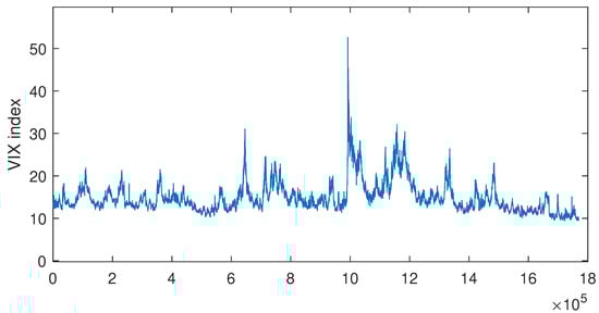
Figure 1.
Plot of 15-s VIX index from 19 March 2013 to 21 July 2017.
Based on the interpolated index, we transformed the non-stationary intraday VIX index into daily curves of cumulative intraday returns (CIDR). Let denote the daily VIX value at time () on day i (); CIDRs are computed by
where denotes the natural logarithm and and are 15-s apart. The daily curves of the CIDR of the VIX index are the functional time series of interest. Figure 2 plots the functional time series curves of the CIDR VIX index for different trading days. From the plot, we can see that there are some variations in the curves for the CIDR VIX index on different trading curves. In fact, on some trading days, the qualitative behaviors of the curves of the CIDR VIX index are different from those on other trading days. For example, the curve of the CIDR VIX index on a trading day between 5 August 2015 and 12 October 2016 exhibits a U-shaped behavior. However, on most of the other trading days, this U-shaped pattern is absent or not so obvious.
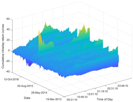
Figure 2.
Plot of functional time series curves of CIDR VIX index from 19 March 2013 to 21 July 2017.
The candidate models we consider to fit the daily curves of the CIDR VIX index are the fAR(1) and fGARCH models. We use the R package ’far’ to fit the observed data to the fAR(1) model. The estimation procedure for fitting the fGARCH model is described in Rice et al. (2023) via quasi-likelihood. The VIX index returns estimated from the fAR(1) model and the fitted estimated from the fGARCH model are plotted in Figure 3. By eyeballing the figure, we see that the fAR(1) model captures some features of the original functional time series of the curves of the CIDR VIX index. Furthermore, the estimated conditional standard deviations from the fitted fGARCH model are strictly increasing on each trading day. This makes intuitive sense for the intraday cumulative returns considered.
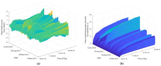
Figure 3.
Plots of fitted functional time series curves of CIDR VIX index from fAR(1) model and fitted conditional standard deviation () from fGARCH model. (a) A plot of fitted daily CIDR VIX index curves from fAR model. (b) A plot of fitted conditional standard deviation from fGARCH model.
To evaluate the adequacy of the fAR(1) model, we apply the functional BDS test on the residuals between the observed returns curves and the fitted return curves (: ; ). Table 7 presents the functional BDS test statistics of the residuals of the fAR(1) model for a variety combination of hyperparameters m and r. Since most test statistics exceed the 1% critical value of a standard normal distribution, the functional BDS test rejects the null hypothesis of IID residuals. In other words, the fAR(1) model cannot capture all the structures underlying the observed daily curves of VIX returns.
Table 7.
The functional BDS test statistics of fAR residuals and fGARCH logarithm squared standardized returns fitted to daily curves of the CIDR VIX index. * indicates the independent null hypothesis is rejected at 5% significance, and ** indicates rejection at 1% significance.
Since the fGARCH is a multiplicative model, we use the standardized returns () to evaluate its adequacy. In the univariate case, when evaluating the adequacy of the GARCH model, if the BDS test is applied directly to the standardized returns , previous studies (see Brock et al. 1991) suggest that the BDS statistic needs to be adjusted to have the right size. Fernandes and Preumont (2012) proposed to apply the BDS test on natural logarithms of squared standardized residuals [] so that the logarithmic transformation casts the GARCH model into a linear additive model. Table 7 records the functional BDS test statistics of the logarithm of the squared standardized returns. From the table, we see that the two models, namely fAR(1) and fGARCH, are rejected in most cases.
To compare the performance of the functional BDS test with the GK test as a model specification test in empirical analysis, Table 8 documents the p-value of the GK independence test for and on the fitted residuals after fAR(1) and standardized returns after fGARCH. In Gabrys and Kokoszka (2007b), the authors investigated the finite-sample performance of the GK independence test with and and concluded that the test power against the fAR(1) model is very good if is used. Since the optimal parameters of the GK test depend on the underlying dynamic of the residuals, which is unknown in empirical studies, we also extend the GK test with relatively larger H and p.
Table 8.
The GK test p-value of fAR residuals and fGARCH standardized returns fitted to daily curves of the CIDR VIX index. ** indicates the independent null hypothesis is rejected at 5% significance, and ** indicates rejection at 1% significance.
Comparing the inferences drawn from the functional BDS test and the GK test provides additional insights into the dynamics of the CIDR VIX functional time series. Based on the functional BDS test results, both the fAR and fGARCH models are insufficient to capture the temporal structure exhibited in the daily CIDR curves of the VIX index. However, the GK test showed evidence of a violation of independence only for the fAR(1) model when a larger p is selected. This indicates that the fGARCH model better fits the observed curves compared to the fAR(1) model. Additionally, the seemingly contradictory conclusions regarding the fGARCH residuals from the functional BDS test and the GK test indicate a nonlinear structure exhibited in the daily curves of the CIDR VIX index. Furthermore, the GK test results indicate that the test’s inference can vary based on the parameters selected, whereas our functional BDS test provides consistent inferences across different parameter selections. This reliable statistical inference forms the foundation for modeling and forecasting VIX returns, which play a crucial role in risk management.
5. Conclusions
In this paper, we extended the BDS test to functional time series. Just like the BDS test in the univariate case, the functional BDS test enjoys some key desired properties, making it a plausible candidate for testing model specification and nonlinearity. Those advantages include a minimal requirement of prior assumptions and knowledge and the capacity to detect linear and nonlinear structures. We proved that the asymptotic normality previously held for the test statistics under the null hypothesis in the univariate case remains valid after extending the test statistics to the functional case. Additionally, we conducted Monte-Carlo experiments on the functional BDS test to provide the recommended range of its hyperparameters and data length. Outside our recommended ranges, the functional BDS test results can be sensitive to the choices of hyperparameters. This aligns with the findings of the conventional BDS test. We showed that with appropriate selection of the hyperparameters, the functional BDS test only required the data to be of length 250 to ensure that they converge to normality and has a 100% correct rate in terms of detecting predictability in a simulated functional time series with a relatively weak temporal structure. Moreover, if either or is selected as a distance measure inside the sup-norms, the function BDS test is also robust to outliers. The code for the functional BDS test is available at https://github.com/Landy339/functional_BDS_test (accessed on 12 December 2024).
We illustrate the significance of our research in an empirical analysis, where we used the functional BDS test to evaluate the adequacy of the fAR model and the fGARCH model in terms of fitting a functional time series to the CIDR VIX index. After fitting the candidate models, we applied the functional BDS test to detect the remaining structures in the residuals. The test rejects the independence null hypothesis and thus concludes that both fAR and fGARCH models are insufficient to capture the temporal structures exhibited in the observed curves fully. In addition, our test showed added sensitivity in detecting predictability, particularly for the nonlinear structure, compared to the existing independence test in functional time series. We compared the results from the functional BDS test with those from the GK test, an existing linear independent test in the domain of functional time series. The results showed that our newly proposed functional BDS test provides a remedy to the weakness of the GK test by detecting the nonlinear structure in the fGARCH residuals that the GK test neglects. With the new tool, one could be aware of the existing independence test that the fGARCH is an adequate model for the observed data and overlook its nonlinear temporal structures.
The functional BDS test is the first nonlinearity test and the first model specification test proposed in functional time series. However, the major limitation of the proposed test is that it can only detect the remaining structures in the residuals. Unfortunately, it cannot indicate the form of the detected structures. Consequently, if a model is deemed insufficient, practitioners have no guidance on what models can fully capture the structures in the observed data.
We conclude by highlighting several potentially interesting issues that may be considered by extending the results obtained in this paper. (1) We provide a range of plausible tuning parameters, with the identification of optimal parameters for specific data sets left as future work. (2) Although our study demonstrated that with the proper selection of norms, the functional BDS test is robust to outliers, future research can examine its behavior on non-stationary functional time series, which frequently arise in real-world data. (3) The current study focused on univariate functional time series. Future work could investigate the extension of nonlinearity tests to multivariate functional time series while accounting for potential correlations among the variables. (4) Since our empirical analysis indicates the existence of nonlinearity in financial functional time series, it is hoped that the proposed test and the respective results will inspire further research into the dependence structure of functional time series, particularly in analyzing, modeling, and forecasting nonlinear functional time series. (5) We demonstrated the use of the BDS test via the 15-s VIX data. We could apply the functional BDS test to other climate or biomedical data sets.
The functional BDS test proposed in this paper provides market practitioners in banks, financial institutions, insurance companies, and regulatory bodies with a theoretically sound and practically feasible way to detect nonlinearity in financial data and model building relevant to risk management. Specifically, we illustrate, using empirical data on the VIX index, how the proposed functional BDS test may be used to detect nonlinearity in the VIX index data and model building for a (forward-looking) risk indicator. The proposed test provides market professionals with a rigorous way to assess the suitability and reliability of their models in managing portfolio risk and diversification, as well as in constructing investment strategies.
Author Contributions
Conceptualization, X.H., H.L.S. and T.K.S.; Methodology, X.H., H.L.S. and T.K.S.; Software, X.H. and H.L.S.; Validation, X.H. and H.L.S.; Formal analysis, X.H. and T.K.S.; Investigation, X.H., H.L.S. and T.K.S.; Resources, H.L.S.; Data curation, X.H. and H.L.S.; Writing—original draft, X.H.; Writing—review and editing, H.L.S. and T.K.S.; Visualization, X.H.; Supervision, H.L.S. and T.K.S.; Project administration, H.L.S.; Funding acquisition, H.L.S. All authors have read and agreed to the published version of the manuscript.
Funding
This research was funded by Australian Research Council, grant number DP230102250.
Data Availability Statement
Dataset available on request from the authors.
Acknowledgments
The authors are grateful for the insightful comments and suggestions of the reviewers, as well as Yuqian Zhao from the University of Sussex for generously sharing his code for part of the empirical studies.
Conflicts of Interest
Xin Huang is employed by Commonwealth Bank of Australia and the authors declare no conflicts of interest.
Appendix A. Additional Monte-Carlo Simulation Results
In Table A1, we present the p-value of the KS test on the functional BDS test statistics computed on simulated IID functional time series with norm and norm being used as the distance measure inside the sup-norms.
Table A1.
The p-value of the KS test on functional BDS test statistics with norm and norm computed on 200 paths of 500 simulated IID functional time series. A p-value less than 0.025 is highlighted in bold, indicating the generated BDS test statistics cannot be assumed to follow a standard normal distribution at the 5% significance.
| m | ||||||||||
|---|---|---|---|---|---|---|---|---|---|---|
| Metric | 2 | 3 | 4 | 5 | 6 | 7 | 8 | 9 | 10 | |
| 0.00 | 0.00 | 0.00 | 0.00 | 0.00 | 0.00 | 0.00 | 0.00 | 0.00 | ||
| 0.00 | 0.00 | 0.00 | 0.00 | 0.00 | 0.00 | 0.00 | 0.00 | 0.00 | ||
| 0.00 | 0.46 | 0.04 | 0.00 | 0.00 | 0.00 | 0.00 | 0.00 | 0.00 | ||
| s.d. | 0.78 | 0.55 | 0.14 | 0.04 | 0.08 | 0.17 | 0.03 | 0.03 | 0.00 | |
| 0.89 | 0.19 | 0.94 | 0.26 | 0.00 | 0.03 | 0.00 | 0.00 | 0.00 | ||
| 0.78 | 0.15 | 0.03 | 0.03 | 0.22 | 0.01 | 0.03 | 0.00 | 0.00 | ||
| 0.24 | 0.30 | 0.74 | 0.15 | 0.00 | 0.57 | 0.08 | 0.02 | 0.27 | ||
| 0.54 | 0.09 | 0.21 | 0.09 | 0.01 | 0.10 | 0.01 | 0.22 | 0.03 | ||
| 0.00 | 0.00 | 0.00 | 0.00 | 0.00 | 0.00 | 0.00 | 0.00 | 0.00 | ||
| 0.09 | 0.00 | 0.00 | 0.00 | 0.00 | 0.00 | 0.00 | 0.00 | 0.00 | ||
| 0.10 | 0.19 | 0.29 | 0.01 | 0.00 | 0.00 | 0.00 | 0.00 | 0.00 | ||
| s.d. | 0.00 | 0.53 | 0.82 | 0.20 | 0.03 | 0.03 | 0.00 | 0.00 | 0.00 | |
| 0.41 | 0.83 | 0.98 | 0.58 | 0.01 | 0.11 | 0.00 | 0.34 | 0.00 | ||
| 0.72 | 0.29 | 0.72 | 0.17 | 0.12 | 0.25 | 0.09 | 0.02 | 0.01 | ||
| 0.86 | 0.03 | 0.53 | 0.40 | 0.22 | 0.02 | 0.35 | 0.11 | 0.00 | ||
| 0.00 | 0.16 | 0.29 | 0.13 | 0.91 | 0.17 | 0.22 | 0.93 | 0.00 | ||
In Table A2, we present the size of the functional BDS test at 5% and 10% nominal levels when is selected as the norm.
Table A2.
The size of the functional BDS test with norm at 5% and 10% nominal levels computed on 200 paths of 500 simulated IID functional time series. The cells with size of the test exceeding the nominal level by 3% are highlighted in bold.
Table A2.
The size of the functional BDS test with norm at 5% and 10% nominal levels computed on 200 paths of 500 simulated IID functional time series. The cells with size of the test exceeding the nominal level by 3% are highlighted in bold.
| Nominal | m | |||||||||
|---|---|---|---|---|---|---|---|---|---|---|
| Level | 2 | 3 | 4 | 5 | 6 | 7 | 8 | 9 | 10 | |
| 71% | 100% | 100% | 100% | 97% | 53% | 12% | 2% | 0% | ||
| 19% | 33% | 61% | 97% | 100% | 100% | 83% | 28% | 3% | ||
| 7% | 11% | 16% | 26% | 38% | 57% | 97% | 100% | 70% | ||
| s.d. | 3% | 10% | 6% | 10% | 10% | 10% | 19% | 30% | 43% | |
| 6% | 9% | 9% | 7% | 6% | 8% | 7% | 7% | 13% | ||
| 4% | 6% | 5% | 4% | 3% | 5% | 5% | 7% | 4% | ||
| 5% | 11% | 11% | 6% | 5% | 9% | 6% | 5% | 9% | ||
| 5% | 9% | 7% | 10% | 9% | 6% | 9% | 8% | 5% | ||
| 76% | 100% | 100% | 100% | 100% | 84% | 37% | 6% | 1% | ||
| 24% | 41% | 67% | 97% | 100% | 100% | 99% | 69% | 18% | ||
| 14% | 19% | 23% | 33% | 47% | 61% | 98% | 100% | 98% | ||
| s.d. | 8% | 14% | 9% | 15% | 18% | 18% | 28% | 39% | 53% | |
| 12% | 13% | 14% | 17% | 9% | 14% | 12% | 14% | 17% | ||
| 8% | 12% | 9% | 9% | 9% | 10% | 12% | 13% | 7% | ||
| 10% | 18% | 15% | 12% | 11% | 14% | 11% | 9% | 12% | ||
| 13% | 16% | 15% | 18% | 15% | 13% | 17% | 16% | 11% | ||
In Table A3, we present the probability that the functional BDS test successfully rejects the IID hypothesis on a structured process when and are selected as the norms.
Table A3.
The successful rejection rate of the functional BDS test on 200 paths of the simulated fGARCH process of 500 observations with and being used as the norm inside the sup-norms and different choices of m and r. NA indicates the select r is too small which leads to every term in (8) being equal to zero, hence the zero denominator in the computed BDS test statistics.
| m | ||||||||||
|---|---|---|---|---|---|---|---|---|---|---|
| Metric | 2 | 3 | 4 | 5 | 6 | 7 | 8 | 9 | 10 | |
| NA | 74% | 61% | NA | 59% | NA | 52% | 1% | NA | ||
| 97% | 85% | 80% | 100% | 97% | 21% | 0% | 0% | 0% | ||
| 99% | 98% | 97% | 89% | 77% | 71% | 71% | 94% | 91% | ||
| s.d. | 95% | 95% | 91% | 91% | 82% | 80% | 74% | 68% | 70% | |
| 93% | 92% | 90% | 82% | 82% | 82% | 68% | 66% | 59% | ||
| 89% | 88% | 84% | 77% | 73% | 74% | 71% | 64% | 59% | ||
| 81% | 78% | 81% | 76% | 77% | 74% | 69% | 63% | 61% | ||
| 82% | 81% | 82% | 74% | 72% | 62% | 60% | 65% | 57% | ||
| NA | NA | NA | NA | NA | NA | NA | NA | NA | ||
| 100% | 99% | 27% | 3% | 0% | 0% | 0% | 0% | 0% | ||
| 97% | 90% | 77% | 100% | 95% | 11% | 1% | 0% | 0% | ||
| s.d. | 100% | 100% | 98% | 93% | 88% | 84% | 79% | 94% | 77% | |
| 100% | 100% | 99% | 98% | 99% | 97% | 94% | 93% | 86% | ||
| 100% | 100% | 99% | 98% | 98% | 96% | 97% | 92% | 91% | ||
| 99% | 100% | 100% | 98% | 97% | 93% | 93% | 95% | 91% | ||
| 99% | 98% | 99% | 98% | 96% | 94% | 94% | 92% | 90% | ||
Table A4 stores the p-value of the KS test on the functional BDS test statistics computed on simulated IID functional time series with 1% random outliers when , , and are used as the norm inside the sup-norms.
Table A4.
The p-value of the KS test on functional BDS test statistics with , , and norms computed on 200 paths of 500 simulated IID functional time series with 1% random outliers. A p-value less than 0.025 is highlighted in bold, indicating that the generated BDS test statistics cannot be assumed to follow a standard normal distribution at the 5% significance.
| m | ||||||||||
|---|---|---|---|---|---|---|---|---|---|---|
| Metric | 2 | 3 | 4 | 5 | 6 | 7 | 8 | 9 | 10 | |
| 0.00 | 0.00 | 0.00 | 0.00 | 0.00 | 0.00 | 0.00 | 0.00 | 0.00 | ||
| 0.05 | 0.00 | 0.00 | 0.00 | 0.00 | 0.00 | 0.00 | 0.00 | 0.00 | ||
| 0.33 | 0.05 | 0.00 | 0.00 | 0.00 | 0.00 | 0.00 | 0.00 | 0.00 | ||
| s.d. | 0.68 | 0.25 | 0.39 | 0.25 | 0.03 | 0.00 | 0.00 | 0.00 | 0.00 | |
| 0.36 | 0.37 | 0.02 | 0.16 | 0.03 | 0.17 | 0.02 | 0.12 | 0.00 | ||
| 0.80 | 0.12 | 0.93 | 0.09 | 0.15 | 0.43 | 0.98 | 0.02 | 0.09 | ||
| 0.40 | 0.70 | 0.76 | 0.16 | 0.85 | 0.21 | 0.49 | 0.42 | 0.01 | ||
| 0.83 | 0.17 | 0.13 | 0.02 | 0.28 | 0.05 | 0.26 | 0.67 | 0.08 | ||
| 0.00 | 0.00 | 0.00 | 0.00 | 0.00 | 0.00 | 0.00 | 0.00 | 0.00 | ||
| 0.01 | 0.00 | 0.00 | 0.00 | 0.00 | 0.00 | 0.00 | 0.00 | 0.00 | ||
| 0.33 | 0.00 | 0.00 | 0.00 | 0.00 | 0.00 | 0.00 | 0.00 | 0.00 | ||
| s.d. | 0.67 | 0.30 | 0.08 | 0.00 | 0.00 | 0.00 | 0.00 | 0.00 | 0.00 | |
| 0.62 | 0.23 | 0.10 | 0.23 | 0.15 | 0.00 | 0.00 | 0.00 | 0.00 | ||
| 0.57 | 0.95 | 0.07 | 0.15 | 0.35 | 0.05 | 0.00 | 0.11 | 0.00 | ||
| 0.18 | 0.35 | 0.49 | 0.19 | 0.01 | 0.31 | 0.03 | 0.01 | 0.23 | ||
| 0.01 | 0.16 | 0.16 | 0.03 | 0.02 | 0.19 | 0.33 | 0.26 | 0.01 | ||
| 0.00 | 0.00 | 0.00 | 0.00 | 0.00 | 0.00 | 0.00 | 0.00 | 0.00 | ||
| 0.00 | 0.00 | 0.00 | 0.00 | 0.00 | 0.00 | 0.00 | 0.00 | 0.00 | ||
| 0.44 | 0.00 | 0.00 | 0.00 | 0.00 | 0.00 | 0.00 | 0.00 | 0.00 | ||
| s.d. | 0.71 | 0.09 | 0.00 | 0.00 | 0.00 | 0.00 | 0.00 | 0.00 | 0.00 | |
| 0.47 | 0.54 | 0.00 | 0.00 | 0.00 | 0.00 | 0.00 | 0.00 | 0.00 | ||
| 0.03 | 0.71 | 0.00 | 0.00 | 0.00 | 0.00 | 0.00 | 0.00 | 0.00 | ||
| 0.17 | 0.08 | 0.00 | 0.00 | 0.00 | 0.00 | 0.00 | 0.00 | 0.00 | ||
| 0.35 | 0.00 | 0.00 | 0.00 | 0.00 | 0.00 | 0.00 | 0.00 | 0.00 | ||
Appendix B. Asymptotic Normality for the BDS Test Statistic and Its Proof
In Section 2, we adjust the specification of the BDS test statistic to be adaptive to the functional case. We prove that the asymptotic normality for the univariate BSD test statistic holds for the functional case. Firstly, we shall provide some mathematical preliminaries relevant to the asymptotic normality result. Then, the BDS test statistic is related to a generalized U statistic with order 2. Finally, the asymptotic normality result and its proof are presented. It is worth noting that the following proof is not restricted by any distance measure when computing sup-norms.
Appendix B.1. Mathematical Preliminaries
The notation and definitions to be presented here follow those in Bosq (1999). Let be a separable Hilbert space with the inner product and the norm . We equip with its Borel -field . Since is a linear metric space with a countable basis, it is a topological space with a countable basis for its topology. By Proposition 3.1 of Preston (2008), since is the Borel -field of generated by Borel subsets of , the measurable space is countably generated. Let be a complete probability space. We consider a discrete-time functional time series on with values in the countably generated measurable space , where is the set of integers. Note that the condition that the state space of a stochastic process is a countably generated measurable space was imposed in Denker and Keller (1983), in which some asymptotic normality results for U-statistics were presented. We shall use the asymptotic results for U statistics to prove the asymptotic normality of the BDS test statistic here. Consequently, we also impose the condition that takes on values in the countably generated measurable space . As in the univariate case of Brock et al. (1996), it is assumed that is a strictly stationary stochastic process. Let be a measure on which is induced by the random element , (i.e., an -valued random variable), under the measure . That is, for any ,
where . Note that is also called an image measure of under the measurable map (see, e.g., Prakasa Rao 2014).
Under the assumption that a strictly stationary stochastic process, the image measure is time-invariant. Therefore, we write for . Let . Note that is a generalization of the m-history in Brock et al. (1996) from the univariate case to the functional case. When are independent under the measure , we consider the m-product to be a countably generated measurable space . In this case, the image measure of under on is given as follows:
for any . Since is time invariant, we write for .
For each with , let be the -augmentation of the -field generated by the set of -valued random elements . Then, according to Volkonski and Rozanov (1961), Grassberger and Procaccia (1983), and Brock et al. (1996), the -valued stochastic process is said to be absolutely regular if
converges to zero as , where is the set of natural numbers.
For each , we consider the max-norm defined by:
where and is the norm on . For the numerical implementation of the BDS test in the functional case, we consider the space (i.e., the space of square-integrable -valued random elements under the measure ). The notation follows that in Bosq (1999). Note that is the space of -valued random elements on with the following norm:
In this case, the max-norm in (A4) becomes
Here, we attempt to prove the asymptotic normality results for the BDS test statistic in the functional case for the general case of the max-norm in (A4).
Let be the characteristic function of a set A. In particular, when , its characteristic function is, for simplicity, denoted by , for any . We now extend the correlation integral in Grassberger and Procaccia (1983) to the case of functional time series. Specifically, the correlation integral for the functional time series at embedding dimension m is defined as follows:
As noted in Brock et al. (1996), under the assumption that is a strictly stationary stochastic process that is regular, the limit expressed as exists, and it is denoted by
In the case of the functional time series, the limit in (A8) is given by
When is an independent process,
Consequently, using (A2) and (A10), (A9) becomes
Write for . Then, from (A11),
Appendix B.2. Generalized U Statistic with Order 2
In the sequel, some concepts of a generalized U statistic with order 2 for the functional time series are presented. The notion of U-statistic may be dated back to Hoeffding (1948). Here, we extend the generalized U statistic in Serfling (1980), and Brock et al. (1996) to the case of functional time series. The expositions here follow those in Denker and Keller (1983) and Brock et al. (1996).
Since is a countably generated measurable space, the (finite) product space is also a countably generated measurable space. Let be a measurable function , for . The measurable function h is called a kernel for the integral:
if h is symmetric in its arguments and . That is,
Then a generalized U-statistic with order 2 is given by
Note that
Then is a symmetric kernel for the integral in (A9). Consequently, by taking in (A16) as , the correlation integral in (A7) coincides with (A16). Therefore, the correlation integral in (A7) is a generalized U-statistic with order 2 and symmetric kernel . Extending the definition in Brock et al. (1996) to the case of functional time series, we define
The last equality follows symmetry. Then,
Consequently,
Appendix B.3. Asymptotic Normality and Its Proof
To establish the asymptotic normality results for the generalized U statistic with order 2 in (A16), as in Brock et al. (1996), we focus on the non-degenerate case where .
To simplify the notation, as in Brock et al. (1996), we write K for and C for unless otherwise stated. Define as follows:
The following theorem gives the first asymptotic normality result, which extends Brock et al. (1996, Theorem 2.1) to the case of functional time series.
Theorem A1.
Suppose that
- 1.
- is a sequence of IID -valued random elements;
- 2.
- .
Then the standardized generalized U statistic with order 2 defined as follows:
converges in distribution to , (i.e., a standard normal distribution with zero mean and unit variance), as , where is given by (A25).
Proof.
The proof follows from Theorem 1(c) in Denker and Keller (1983) and the proof of Theorem 2.1 in Brock et al. (1996). Here, we consider the -valued stochastic process on the probability space . Under Condition 1 that are IID, and are independent if . Then, the two -fields and , for , must be independent. Then, for any with ,
Consequently, for each , in (A3) must be identical to zero. This implies that is absolutely regular. Since it was assumed that is a strictly stationary -valued process, is an absolutely regular strictly stationary -valued process. Since , for all , and , for all , , for some . Note that . Then
Consequently, the conditions in Denker and Keller (1983, Theorem 1(c)) are fulfilled. This then establishes the convergence of the standardized generalized U statistic with order 2 in (A26) in distribution to a standard normal distribution. It remains to prove that is given by (A25). Define, for each ,
For each , let be the component of . Under Condition 1,
Using the asymptotic variance from Denker and Keller (1983) and writing for ,
From (A29),
Taking expectation in (A36) gives the following:
To evaluate , two cases are considered, namely and .
Recall that and . Then, for , the overlapping elements of and are . The non-overlapping elements are as follows:
Consequently, for ,
Note that
and that
Therefore, using (A44), (A47) and (A48), for ,
For , and are independent because they do not have overlapping terms. Using this fact and (A31),
Consequently, using (A35), (A38), (A54), and (A55),
This then gives the asymptotic variance in (A25) and completes the proof. □
Note
| 1 | To explain the sup-norm or the -norm, we first need to consider the notion of essential supremum. Let denote a measure space, where is a measurable space and l is the Lebesgue measure. Let f denote a real-valued measurable function on X, say . Then, the essential supremum of the function f over the space X is defined by: |
References
- Aue, Alexander, Lajos Horváth, and Daniel F. Pellatt. 2017. Functional generalized autoregressive conditional heteroskedasticity. Journal of Time Series Analysis 38: 3–21. [Google Scholar] [CrossRef]
- Bosq, Denis. 1991. Modelization, nonparametric estimation and prediction for continuous time processes. In Nonparametric Functional Estimation and Related Topics. Berlin/Heidelberg: Springer, pp. 509–29. [Google Scholar]
- Bosq, Denis. 1999. Autoregressive Hilbertian processes. Annales de l’ISUP, Publications de l’Institut de Statistique de l’Université de Paris XXXXIII: 25–55. [Google Scholar]
- Brock, William A. 1987. Notes on Nuisance Parameter Problems in BDS Type Tests for IID. Unpublished manuscript. Madison: University of Wisconsin. [Google Scholar]
- Brock, William A., David Arthur Hsieh, and Blake Dean LeBaron. 1991. Nonlinear Dynamics, Chaos, and Instability: Statistical Theory and Economic Evidence. Cambridge and London: MIT Press. [Google Scholar]
- Brock, William A., José Alexandre Scheinkman, W. Davis Dechert, and Blake LeBaron. 1996. A test for independence based on the correlation dimension. Econometric Reviews 15: 197–235. [Google Scholar] [CrossRef]
- Brock, William A., W. Davis Dechert, and José Alexandre Scheinkman. 1987. A Test for Independence Based on the Correlation Dimension. Working Paper. Madison: Department of Economics, University of Wisconsin at Madison. Houston: University of Houston. Chicago: University of Chicago. [Google Scholar]
- Caporale, Guglielmo Maria, Christos Ntantamis, Theologos Pantelidis, and Nikitas Pittis. 2005. The BDS test as a test for the adequacy of a GARCH(1,1) specification: A Monte Carlo study. Journal of Financial Econometrics 3: 282–89. [Google Scholar] [CrossRef][Green Version]
- Chan, Kung-Sik, and Howell Tong. 2001. Chaos: A Statistical Perspective. New York: Springer Science & Business Media. [Google Scholar]
- Chiou, Jeng-Min, and Hans-Georg Müller. 2007. Diagnostics for functional regression via residual processes. Computational Statistics & Data Analysis 51: 4849–63. [Google Scholar]
- Damon, Julien, and Serge Guillas. 2002. The inclusion of exogenous variables in functional autoregressive ozone forecasting. Environmetrics 13: 759–74. [Google Scholar] [CrossRef]
- de Lima, Pedro J. F. 1996. Nuisance parameter free properties of correlation integral based statistics. Econometric Reviews 15: 237–59. [Google Scholar] [CrossRef]
- Denker, Manfred, and Gerhard Keller. 1983. On U-statistics and v. mises’ statistics for weakly dependent processes. Zeitschrift für Wahrscheinlichkeitstheorie und Verwandte Gebiete 64: 505–22. [Google Scholar] [CrossRef]
- Escot, Lorenzo, Julio E. Sandubete, and Łukasz Pietrych. 2023. Detecting structural changes in time series by using the BDS test recursively: An application to COVID-19 effects on international stock markets. Mathematics 11: 4843. [Google Scholar] [CrossRef]
- Fernandes, Marcelo, Marcelo C. Medeiros, and Marcel Scharth. 2014. Modeling and predicting the CBOE market volatility index. Journal of Banking & Finance 40: 1–10. [Google Scholar]
- Fernandes, Marcelo, and Pierre-Yves Preumont. 2012. The finite-sample size of the BDS test for GARCH standardized residuals. Brazilian Review of Econometrics 32: 241–60. [Google Scholar] [CrossRef][Green Version]
- Gabrys, Robertas, and Piotr Kokoszka. 2007b. Portmanteau test of independence for functional observations. Journal of the American Statistical Association: Theory and Methods 102: 1338–48. [Google Scholar] [CrossRef]
- García-Portugués, Eduardo, Javier Álvarez-Liébana, and Gonzalo Álvarez-Pérez. 2019. A goodness-of-fit test for the functional linear model with functional response. Scandinavian Journal of Statistics 48: 502–28. [Google Scholar] [CrossRef]
- González, José Portela, Antonio Muñoz San Muñoz San Roque, and Estrella Alonso Perez. 2017. Forecasting functional time series with a new Hilbertian ARMAX model: Application to electricity price forecasting. IEEE Transactions on Power Systems 33: 545–56. [Google Scholar] [CrossRef]
- Grassberger, Peter, and Itamar Procaccia. 1983. Characterization of strange attractors. Physical Review Letters 50: 346. [Google Scholar] [CrossRef]
- Hoeffding, Wassily. 1948. A class of statistics with asymptotically normal distribution. Annals of Mathematical Statistics 19: 293–325. [Google Scholar] [CrossRef]
- Horváth, Lajos, Marie Hušková, and Gregory Rice. 2013. Test of independence for functional data. Journal of Multivariate Analysis 117: 100–19. [Google Scholar] [CrossRef]
- Hörmann, Siegfried, Lajos Horváth, and Ron Reeder. 2013. A functional version of the ARCH model. Econometric Theory 29: 267–88. [Google Scholar] [CrossRef]
- Huang, Xin, and Han Lin Shang. 2023. Nonlinear autocorrelation function of functional time series. Nonlinear Dynamics 111: 2537–54. [Google Scholar] [CrossRef]
- Hyndman, Rob, and Han Lin Shang. 2025. ftsa: Functional Time Series Analysis. R Package Version 6.5. Available online: https://cran.r-project.org/web/packages/ftsa/ (accessed on 19 January 2025).
- Kim, Hae Sung, Doosun Kang, and Joong Hoon Kim. 2003. The BDS statistic and residual test. Stochastic Environmental Research and Risk Assessment 17: 104–15. [Google Scholar] [CrossRef]
- Kim, Mihyun, Piotr Kokoszka, and Gregory Rice. 2023. White noise testing for functional time series. Statistics Surveys 17: 119–68. [Google Scholar] [CrossRef]
- Klepsch, Johannes, Claudia Klüppelberg, and Taoran Wei. 2017. Prediction of functional ARMA processes with an application to traffic data. Econometrics and Statistics 1: 128–49. [Google Scholar] [CrossRef]
- Kočenda, Evzen. 2001. An alternative to the BDS test: Integration across the correlation integral. Econometric Review 20: 337–51. [Google Scholar] [CrossRef]
- Kokoszka, Piotr, and Matthew Reimherr. 2017. Introduction to Functional Data Analysis. Boca Raton: Chapman and Hall/CRC. [Google Scholar]
- Kokoszka, Piotr, Gregory Rice, and Han Lin Shang. 2017. Inference for the autocovariance of a functional time series under conditional heteroscedasticity. Journal of Multivariate Analysis 162: 32–50. [Google Scholar] [CrossRef]
- Konstantinidi, Eirini, George Skiadopoulos, and Emilia Tzagkaraki. 2008. Can the evolution of implied volatility be forecasted? Evidence from European and US implied volatility indices. Journal of Banking & Finance 32: 2401–11. [Google Scholar]
- LeBaron, Blake. 1997. A fast algorithm for the BDS statistic. Studies in Nonlinear Dynamics & Econometrics 2: 1. [Google Scholar]
- Lee, Tae-Hwy, Halbert White, and Clive W. J. Granger. 1993. Testing for neglected nonlinearity in time series models: A comparison of neural network methods and alternative tests. Journal of Econometrics 56: 269–90. [Google Scholar] [CrossRef]
- Luo, Wenya, Zhidong Bai, Shurong Zheng, and Yongchang Hui. 2020. A modified BDS test. Statistics & Probability Letters 164: 108794. [Google Scholar]
- Mammadli, Sadig. 2017. Analysis of chaos and nonlinearities in a foreign exchange market. Procedia Computer Science 120: 901–7. [Google Scholar] [CrossRef]
- Mestre, Guillermo, José Portela, Gregory Rice, Antonio Muñoz San Roque, and Estrella Alonso. 2021. Functional time series model identification and diagnosis by means of auto-and partial autocorrelation analysis. Computational Statistics & Data Analysis 155: 107108. [Google Scholar]
- Packard, Norman H., James P. Crutchfield, J. Doyne Farmer, and Robert S. Shaw. 1980. Geometry from a time series. Physical Review Letters 45: 712. [Google Scholar] [CrossRef]
- Prakasa Rao, B. L. S. 2014. Characterization of Gaussian distribution on a Hilbert space from samples of random size. Journal of Multivariate Analysis 132: 209–14. [Google Scholar] [CrossRef]
- Preston, Chris. 2008. Some notes on standard Borel and related spaces. arXiv arXiv:0809.3066. [Google Scholar]
- Rice, Gregory, Tony Wirjanto, and Yuqian Zhao. 2023. Exploring volatility of crude oil intra-day return curves: A functional GARCH-X model. Journal of Commodity Markets 32: 100361. [Google Scholar] [CrossRef]
- Rudin, Walter. 1987. Real and Complex Analysis. Singapore: McGRaw-Hill Book Co. [Google Scholar]
- Serfling, Robert J. 1980. Approximation Theorems of Mathematical Statistics. New York: John Wiley & Sons. [Google Scholar]
- Shang, Han Lin. 2017. Forecasting intraday S&P 500 index returns: A functional time series approach. Journal of Forecasting 36: 741–55. [Google Scholar]
- Shang, Han Lin, Jiguo Cao, and Peijun Sang. 2022. Stopping time detection of wood panel compression: A functional time-series approach. Journal of the Royal Statistical Society: Series C 71: 1205–24. [Google Scholar] [CrossRef]
- Shang, Han Lin, Steven Haberman, and Ruofan Xu. 2022. Multi-population modelling and forecasting life-table death counts. Insurance: Mathematics and Economics 106: 239–53. [Google Scholar] [CrossRef]
- Shang, Han Lin, Yang Yang, and Fearghal Kearney. 2019a. Intraday forecasts of a volatility index: Functional time series methods with dynamic updating. Annals of Operation Research 282: 331–54. [Google Scholar] [CrossRef]
- Small, Michael, and Chi K. Tse. 2003. Determinism in financial time series. Studies in Nonlinear Dynamics & Econometrics 7: 1134. [Google Scholar]
- Takens, Floris. 1981. Detecting strange attractors in turbulence. In Dynamical Systems and Turbulence, Warwick 1980. Edited by D. Rand and Lai-Sang Young. Berlin/Heidelberg: Springer, pp. 366–81. [Google Scholar]
- Tang, Chen, and Yanlin Shi. 2021. Forecasting high-dimensional financial functional time series: An application to constituent stocks in Dow Jones index. Journal of Risk and Financial Management 14: 343. [Google Scholar] [CrossRef]
- Turbillon, Céline, Jean-Marie Marion, and Besnik Pumo. 2007. Estimation of the moving-average operator in a Hilbert space. In Recent Advances in Stochastic Modeling and Data Analysis. Edited by Christos H. Skiadas. Singapore: World Scientific, pp. 597–604. [Google Scholar]
- Volkonski, V. A., and Y. A. Rozanov. 1961. Some limit theorems for random function II. Theory of Probability and Its Applications 6: 186–98. [Google Scholar] [CrossRef]
- Zamani, Atefeh, Hossein Haghbin, Maryam Hashemi, and Rob J Hyndman. 2022. Seasonal functional autoregressive models. Journal of Time Series Analysis 43: 197–218. [Google Scholar] [CrossRef]
- Zhang, Xianyang. 2016. White noise testing and model diagnostic checking for functional time series. Journal of Econometrics 194: 76–95. [Google Scholar] [CrossRef]


Disclaimer/Publisher’s Note: The statements, opinions and data contained in all publications are solely those of the individual author(s) and contributor(s) and not of MDPI and/or the editor(s). MDPI and/or the editor(s) disclaim responsibility for any injury to people or property resulting from any ideas, methods, instructions or products referred to in the content. |
© 2025 by the authors. Licensee MDPI, Basel, Switzerland. This article is an open access article distributed under the terms and conditions of the Creative Commons Attribution (CC BY) license (https://creativecommons.org/licenses/by/4.0/).