Article

Structural Changes in Persistence of Mortality

Mathematics Department, Lebanon Valley College, Annville, PA 17003, USA
*
Author to whom correspondence should be addressed.
Risks 2025, 13(11), 225; https://doi.org/10.3390/risks13110225
Submission received: 8 September 2025 / Revised: 10 November 2025 / Accepted: 13 November 2025 / Published: 18 November 2025

Abstract

Recent researchers have observed that long-memory is prevalent in mortality data. Related to a quantifiable measure of persistence, it is an important characteristic of mortality dynamics. However, prior researchers did not consider potential change in the persistence degree and assumed it is constant. This article for the first time considers change in the persistence of mortality and demonstrates that mortality data displays obvious and substantial such changes. We apply a test of Martins and Rodrigues, a tool that has already been demonstrated to be effective in macroeconomics research, to detect the change in persistence in mortality time series for the first time. Our approach considers changes both in persistence and also in trend, separately, for each single-age mortality time series. Our results show that these two types of structural changes are very different in the aspects of age clustering and the time points of breaks. In experiments on simulated data, our model presents the best accuracy in the estimation of persistence degree compared to two control models.

1. Introduction

Over the last century, many countries experienced a significant mortality improvement, causing increased life expectancy and this has had a great impact on managing pensions, annuities, and other portfolios with mortality risk. Persistence is one important feature of mortality dynamics, which indicates the degree of dependence in the time series, and it can be quantified. For a series with low persistence, when an exogenous shock happens, it will only have transitory effects on the time series, but the value of the persistence affects the time-scale over which shocks dissipate. For a series with high enough persistence, an exogenous shock can have either very long-lived transitory effects or even permanent effects. (For instance, permanent effects can happen with non-stationary series. When it occurs in mortality, policy interventions may be recommended if the shock is negative.) Models with high persistence include those termed long-memory models, which have long been used in econometrics and recently been used to demonstrate the presence of long-memory in some mortality time-series. The long-memory model structure adopted in a mortality model can improve the fitting and forecasting of mortality Yan et al. (2020).
Researchers in macroeconomics have studied changes in persistence of financial variables like inflation rates, trading volume, volatility, and son on (see Kim (2000); Busetti and Taylor (2004); Harvey et al. (2006); Davidson and Monticini (2010); Martins and Rodrigues (2014)). In this paper, for the first time in the mortality field, we considered change in persistence of mortality. It is also the first time the test in Martins and Rodrigues (2014) (MR test), which can capture changes in persistence, has been applied to mortality time series. We find that mortality data also displays obvious changes in persistence.
We illustrate these changes by running our model on the mortality time series for each age in France and Sweden data, and we show that there is a significant portion of the full ages which experienced a structural change in persistence, after removing the structural changes in trend. It would seem obvious that mortality in a country would experience some kind of structural change from time to time, for instance when it is involved in a war. So it is important to recognize here that the new observation in this article, that persistence of series obtained from detrending mortality time series can experience structural change, is less intuitive as that of change in trend. Some exogenous shocks thought to bring structural changes to mortality may only affect the trend but not necessarily the persistence. We also observe that there are factors affecting persistence while not affecting the trend. For now, we defer further discussion to Section 3.2.
To understand better how different types of structural changes behave, we compared the structural change in persistence and the structural changes in trend of mortality in aspects of age clustering and break timepoints. They are obviously different and this supports a model considering them both and separately. Our paper is the first one to make such consideration. Understanding how breaks in persistence change across ages could presumably aid actuaries or policymakers in focusing their decisions on particular populations (see Section 3.2). By testing on simulated data, we also show that our model has the best accuracy in persistence parameter estimation, compared with two other control models.
Mortality literature has paid attention to the degree of persistence or long-memory feature in mortality data in recent decades. Standard unit root tests are used to determine whether the series is stationary or not by checking 0 or 1 for the order of integration, like the augmented Dickey Fuller Test used in Bishai (1995) and the panel unit root test applied in Dreger and Reimers (2005). However, the mortality time series usually is neither “pure” stationary with order 0 integrated I ( 0 ) nor “pure” nonstationary with order 1 integrated I ( 1 ) , but has a fractional persistence degree. By Diebold and Rudebusch (1991); Hassler and Wolters (1994); Lee and Schmidt (1996); Ben Nasr et al. (2014), standard unit tests do not perform well on a fractionally-integrated series. For instance, Bishai (1995) cannot reject the null of there being a unit root for all the Sweden, UK and US infant mortality series in the ADF tests, implying that they are all I ( 1 ) , nonstationary and not mean-reverted. However, more precise information is given in our approach: we find the logarithm of Sweden age-0 mortality show persistence stationary and long-memory, after removing its trend. Therefore, models with fractional persistence have drawn attention in the mortality field recently, like the autoregressive fractionally integrated moving average model Granger and Joyeux (1980); Hosking (1981) and the Gegenbauer autoregressive moving average (GARMA) model Hosking (1981). These have been applied in the mortality context, see Gil-Alana et al. (2017); Caporale and Gil-Alana (2014); Yaya et al. (2018); Yan et al. (2020); Yan et al. (2021). Specifically, Gil-Alana et al. (2017) examines the infant mortality rates for 37 countries and shows significant differences in the degree of persistence among them. Yaya et al. (2018) finds the order of persistence for the under-5 mortality series in G7 countries. They find it is very high for neonatal mortality (persistence 1 , so the series is mean-reverting) for all cases while the opposite for the remaining ages (<1 to <5 years, mean-reversion in many cases). Long memory features are observed prevalently in mortality data for each gender, age and county Yan et al. (2021); Peters et al. (2021). A model incorporating a long memory structure enhances mortality forecasts Yan et al. (2021); Yan et al. (2020). However, these papers only consider an uniform persistence degree over the covered period and haven’t considered the structural change in persistence, which is observed by our model in mortality data.
Trend is allowed in some papers when they model the persistence by unit root tests or fractional persistence models. For example, nonlinear time trends or linear time trends are considered when estimating the fractional order of integration for mortality in Gil-Alana et al. (2017); Yaya et al. (2018); Caporale and Gil-Alana (2014); Yan et al. (2020); Yan et al. (2021) extend the Lee-Carter model Lee and Carter (1992) to death counts considering period and cohort effects and incorporate a generalized linear GARMA model as the long-memory structure. These papers may consider the dynamics like structural changes or nonlinearity in the trend of mortality, but they neglect possible structural change in the persistence degree and assume the persistence degree to be unchanging.
Failure to consider structural breaks in the trend of a time series has been recognized in many contexts to confuse the long-memory estimation for the series, leading to overestimation of the persistence degree, sometimes producing spurious long memory Cheung (1993); Diebold and Inoue (2001); Granger and Hyung (2004); Dreger and Reimers (2005); Gil-Alana et al. (2017). Our paper also observed the overestimation of the constant persistence degree for series with existing structural breaks in trend, when the model doesn’t consider these structural breaks. Literature has realized obvious structural breaks in trend of mortality (see Fu et al. (2022); Fu et al. (2023); Fu et al. (2025); Milidonis et al. (2011); Hainaut (2012); Li et al. (2011); Lundström and Qvist (2004)), as well as the universal long memory features in mortality data. Therefore to model mortality time series, persistence and structural change in trend should be both characterized and dealt with separately. Our model has done so and further considered the structural changes in persistence featured by the MR test.
Our results also demonstrate that the unconsidered structural changes in trend will distort the estimation of the structural change in persistence. The estimated persistence degree in both regimes are notably overestimated and the amount of ages experiencing a change in persistence is also greatly overestimated. Moreover, we observe that the structural changes in trend and structural changes in persistence are very different in the aspects of age clustering and break points. These support our considering both the structural break in persistence and structural breaks in trend of mortality separately in our model. This may explain the superior accuracy of our model in the testing experiments on simulated data compared with other two control models.
Different tests have been proposed to detect changes in persistence for a series in time series literature. The earlier works like Kim (2000); Busetti and Taylor (2004); Leybourne and Taylor (2004); Leybourne et al. (2003); Leybourne et al. (2007) focuse on I ( 0 ) / I ( 1 ) framework, which test the null of either I ( 0 ) or I ( 1 ) against the alternative of a change from either I ( 0 ) to I ( 1 ) or I ( 1 ) to I ( 0 ) . More recent methods are capable of detecting changes from I ( d 1 ) to I ( d 2 ) with d 1 , d 2 allowed to be non-integers—see Hassler and Scheithauer (2011) (with d 1 = 0 ), Sibbertsen and Kruse (2009) and Martins and Rodrigues (2014) (the MR test). Experiments in Martins and Rodrigues (2014) show the MR test compares favorably to the tests in Hassler and Scheithauer (2011); Sibbertsen and Kruse (2009). The MR test also allows both d 1 , d 2 to be fractional and can identify changes from I ( d 1 ) to I ( d 2 ) with d 1 d 2 even not knowing the direction of the change. Because of the good performance and simplicity of the MR test, we choose it as the tool to detect change in persistence in our model.
This paper is organized as follows. Section 2 gives the model formulation, and Section 3 shows the main results of our model. Section 4 concludes.

2. Model Formulation

Granger and Joyeux (1980); Hosking (1981) proposed to use the fractional difference operator in the A R I M A ( p , d , q )  Box and Jenkins (1976) model to explain both the short-term or long-term correlation structure of a time series.
Let L denote the lag-operator, so the difference operator ( 1 L ) d can be defined for any real number d > 1 as
( 1 L ) d = Σ j = 0 Γ ( j d ) Γ ( j + 1 ) Γ ( d ) L j , and Γ ( · ) is the gamma function .
Define an A R I M A ( p , d , q ) process with integers p , q and real number d to be a discrete-time stochastic process { y t } satisfying
ϕ ( L ) ( 1 L ) d y t = θ ( L ) ϵ t ,
where ϵ t is independent identically distributed white noise and ϕ ( L ) , θ ( L ) are polynomials in L with order p and q respectively.
Such a process { y t } is called a fractionally integrated process of order d and can be written as y t I ( d ) . The parameter d is an important indicator of the degree of dependence in the series and represents significant features about its persistence. White noise and the stationary ARMA models are in the I ( 0 ) class. As Hosking (1981) mentions, as lag increases, the effect of d on distant observations decays hyperbolically, much slower than the effect of ϕ , θ parameters decaying exponentially. Therefore the long-term behavior of an A R I M A ( p , d , q ) process would be similar to an A R I M A ( 0 , d , 0 ) with the same d, due to the negligible effects of the ϕ , θ parameters for very distant observations.
In this paper, we only consider the case p = q = 0 , i.e., A R I M A ( 0 , d , 0 ) process, for simplicity. Then the Equation (2) becomes
( 1 L ) d y t = ϵ t .
Different values of the order d represent different persistence features in the correlation structure of the A R I M A ( 0 , d , 0 ) process { y t }1. For example, 0.5 < d < 0 means that { y t } is stationary, anti-persistent and has a short memory; 0 < d < 0.5 indicates stationarity with long memory2; 0.5 < d < 1 means nonstationarity though mean reversion; d 1 implies lack of mean-reversion and permanent effects of disturbances.
In this paper, we applied the test for persistence change devised by Martins and Rodrigues (2014) (MR test) to determine whether a time series shows a structural change in persistence or not. The MR test is capable of detecting changes between fractionally integrated processes with different persistence parameters d.
The MR test considers an A R I M A ( 0 , d t , 0 ) process { y t } t = 1 , 2 , , T . It tests the null of constant d t , i.e., d t = d s against the alternative of a change in d t ’s value from d 1 to d 2 which happens at time [ τ T ] with unknown τ in [ Λ l , 1 Λ l ] [ 0 , 1 ] . Here Λ l is pre-determined and typically is chosen as 0.15 or 0.20 in literature. The details of the MR test like its statistics derivation and the limit distributions are included in the Appendix A.
In our approach (described in Section Check for Change in Persistence on Detrended Mortality Data), we applied the R package memochange (version 1.1.2) Wenger and Becker (2019) to perform the MR test on a detrended mortality time series and estimate the break time point [ τ T ] , d 1 and d 2 if a break occurs.

Check for Change in Persistence on Detrended Mortality Data

We propose a new model to analyze the feature dynamics in persistence as well as in trend of mortality data by considering structural change in persistence and the structural change in linear trend of the logarithm of mortality.
For each age x, we consider the mortality rates m x t for year t { 1 , 2 , , T } and assume this time series satisfies
ln m x t = β x , t I + β x , t S · t + p t ,
where
  • p t is a A R I M A ( 0 , d t , 0 ) process satisfying that ( 1 L ) d t p t is i.i.d. white noise. d t may be a constant d s over the sample or experience a structural change at T d changing from d 1 to d 2 , which can be tested by the MR test.3
  • For each fixed age x, β x , t I + β x , t S · t is a piecewise linear function of t which describes the trend and trend dynamics of ln m x t , t = 1 , 2 , , T . We assume that there are b { 0 , 1 , 2 , , K } (with K predetermined) structural changes in the trend. In other word, b is the number of structural changes in (linear) trend of ln m x t for age x and K is the possible biggest value for b, where b may differ among ages but K is uniformly chosen for all ages considered. If b > 0 , we denote the breakpoints as { T 1 , T 2 , T b } ( T 0 + 1 = 1 , T b + 1 = T ) in ascending order. So β x , t I , β x , t S are step functions of t defined as
    β x , t I = β x , j I and β x , t S = β x , j S if T j < t T j + 1 , for j = 0 , 1 , b ,
    representing the corresponding intercept and slope of the linear trend in the ( j + 1 ) t h segment.
In our approach, for a specific age x, we first fit the structural changes in linear trend of ln m x t , t = 1 , 2 , , T and detrend ln m x t by removing the fitted trend with changes, then apply the MR test on the detrended ln m x t to analyze its persistence change.
To compute the breakpoints in regression relationships and fit the linear trend with changes β x , t I + β x , t S · t , we follow the method described in Zeileis et al. (2003) and use the R package strucchange Zeileis et al. (2002). In our experiments, we set K = 3 , i.e., up to four stages in ln m x t , and choose b { 0 , 1 , 2 , 3 } that minimizes the BIC in the estimation.
After the linear trends with changes in ln m x t is estimated, denoted as β ^ x , t I + β ^ x , t S · t , we remove it from ln m x t to detrend ln m x t and obtain the estimate of p t , denoted as p t ^ . If b ^ = 0 , so for the specific age x there is no structural change found in the linear trend, then the detrending will only remove the fitted simple linear regression of ln m x t ; if b ^ > 0 , then p t ^ = ln m x t [ β ^ x , t I + β ^ x , t S · t ] .
Martins and Rodrigues (2014) recommend to adequately demean or detrend the studied time series before applying their MR test in the context of a A R I M A ( 0 , d t , 0 ) process. So we would like to demonstrate that the p t ^ obtained by our approach is adequately detrended. The CUSUM fixed-m type A test in Wenger et al. (2019) is able to test change in mean in a long-memory time series. We use the Gaussian Semiparametric local Whittle estimator in Robinson (1995) (available in the R package LongMemoryTS Leschinski (2019)) to obtain the estimation of the persistence parameter d ^ G S L W and then applied the CUSUM fixed-m type A test (available in the R package memochange) to test for a change-in-mean in p ^ under d ^ G S L W . If the time series cannot reject the null hypothesis of a constant mean at 5% rejection, we regard it as “detrended adequately”.
We run our model on mortality for France and Sweden separately. For both countries and all ages, after the detrending process described above, every p t ^ for the corresponding age cannot reject the null hypothesis of a constant mean at 5% rejection in the CUSUM fixed-m type A test and is regarded as being detrended adequately. Here, the CUSUM fixed-m type A test with bandwidth 10 (suggested) is uniformly applied on p t ^ for all ages.
Then we apply the MR test to p t ^ to analyze its persistence parameter d t , given that p t is assumed to be A R I M A ( 0 , d t , 0 ) , and the MR test tests whether there is a structural change in d t . In all our experiments, we uniformly apply the squared t-statistic as the test statistic, set Λ l = 0.2 (used in the original paper by Martins and Rodrigues (2014)) and bandwidth 0.7 in the estimation of persistence parameter (recommended by the package), and use the exact local Whittle estimator by Shimotsu and Phillips (2005) to determine d t in the two regimes ( d 1 and d 2 ) if a break occurs. We reject the null hypothesis of d t = d s over the sample at 10 % rejection, and in this case we claim that a structural change happened in persistence. If for a certain p t ^ the null hypothesis cannot be rejected, we claim there is no structural change in persistence and apply the Gaussian Semiparametric local Whittle estimator in Robinson (1995) to estimate the constant d t (i.e., d s ) for it.

3. Main Results

We apply our model to the mortality data of the total population of France during 1816-2022 and the total population of Sweden during 1751–2022, both for ages 0 to 100, which are collected by age and year ( 1 × 1 ) and provided in the Human Mortality Database Human Mortality Database (n.d.) (HMD). Since we want to study the persistence feature of mortality, we choose the two countries with the first two longest periods of available mortality data in the HMD.4
Section 3.1 presents that our model captured the clear existence of structural change in persistence in mortality (after removing the structural changes in trend) for a significant portion of ages, and timepoints of the breaks are also reported. In Section 3.2, we compared the structural changes in persistence and the structural changes in linear trend in mortality from the aspects of age clustering and break timepoints. Their difference supports the need for a careful method to consider them both, and separately. Section 3.3 checks the accuracy of the estimation of persistence when using our model by testing it on simulated data, compared with two other control models. Among the three models, our model performs the best in accuracy for the persistence parameter estimation.

3.1. Captured Structural Change in Persistence for Adequately Detrended Mortality Data

We applied our model (described in Section Check for Change in Persistence on Detrended Mortality Data) to both the total population mortality data in France and in Sweden, with their longest available data period. We started with the time series l n ( m x t ) for each age in 0 to 100 for the whole time period. We first detrended the time series using the method in Section Check for Change in Persistence on Detrended Mortality Data with 3 as the largest possible number of structural changes in linear trends. For the detrended time series, we applied the CUSUM fixed-m type A to it to test any change in mean under long memory. The results show that all the detrended time series cannot reject the null hypothesis of a constant mean at 5% rejection, both for France data and Sweden data. Therefore, we regarded all time series as detrended adequately and performed the MR test on each of them at the 90% significance level, to check whether there is a structural change in persistence in the adequately detrended time series.
Our results show that there are 76.24% ages for France and 43.56% ages for Sweden among ages 0 to 100 which are observed to have a structural change in persistence at some time point.5 This evidence supports that the existence of structural change in persistence of mortality data is obvious and non-negligible.
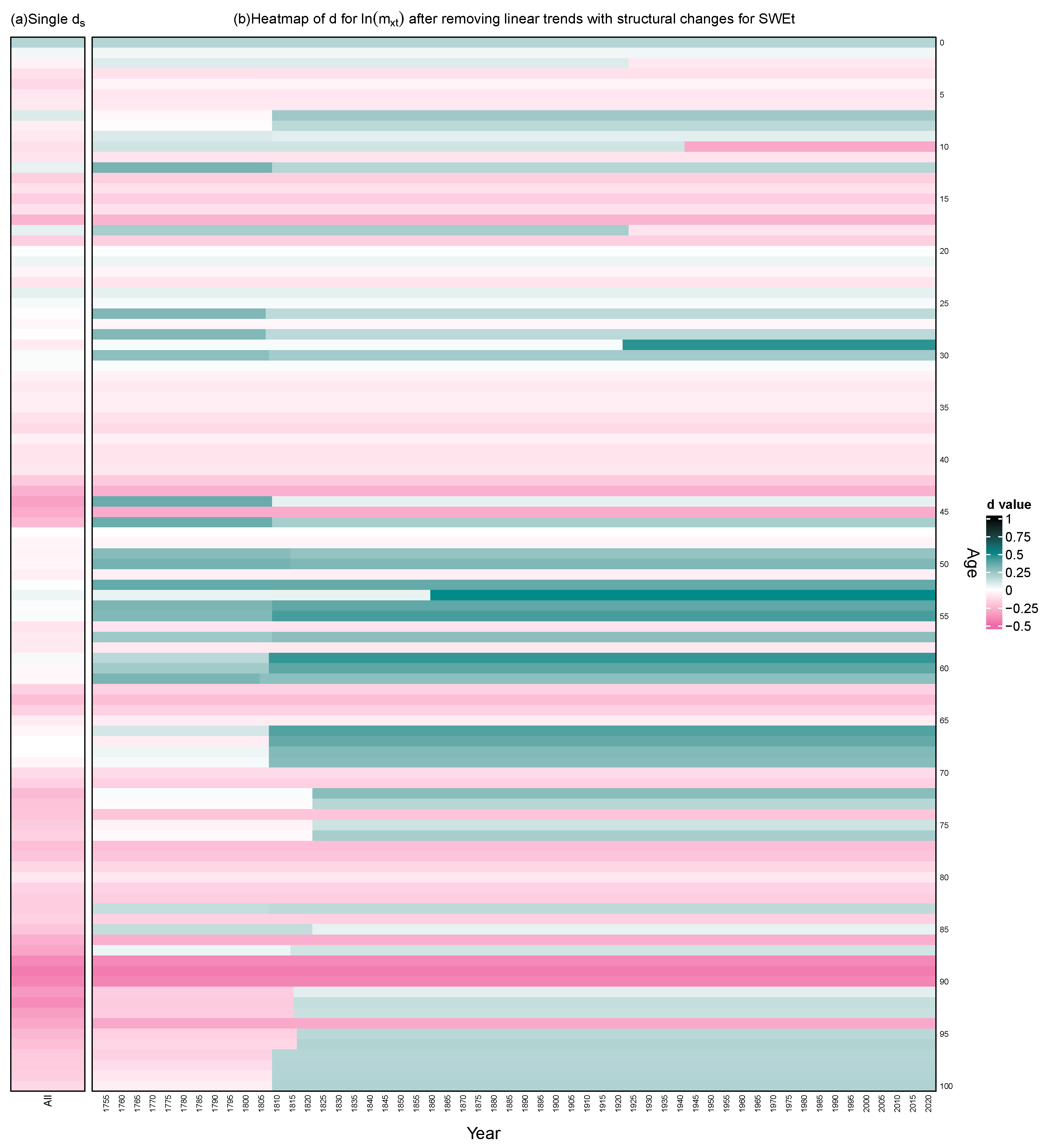
Figure 1b and Figure 2b present the heatmaps of estimated d for each age and year for France data and Sweden data respectively. For any age with observed structural change in persistence, the row will take on two different colors that represent estimated d 1 and d 2 respectively, and the color change point represents the timepoint of the structural change in d. For any age with no observed structural change in persistence, the row will only take on one color that represents the estimated d s value from the Gaussian Semiparametric local Whittle estimator. For example, Figure 1b shows that the age-12 France total population mortality experienced a structural change in persistence in year 1861 (a zoom-in of just age 12 is in Figure 3); before the year 1861, d is estimated to be d 1 = 0.1953 (in pink, anti-persistent and short-memory) and starting from 1861, d is estimated to be d 2 = 0.3035 (in light green, stationary and long-memory).
From the heatmaps, one can notice that there are significant portions of ages presenting structural changes in persistence. Also for the same age, the values of fitted d 1 and d 2 are obviously different. There are changes in d from anti-persistence (in pink) to long memory (in light green) or even to non-stationary random walk (in dark green), from less persistent to more persistent (green getting darker) or in the opposite direction, etc.
Compared to Sweden, France total population has more ages experiencing structural change in persistence and the gap between d 1 and d 2 is usually greater. Sweden’s total population has more anti-persistent (in pink) cases and never has random walk (in dark green) cases.
Figure 1a and Figure 2a also provide the single persistence d s estimated by using the Gaussian Semiparametric local Whittle estimator on the adequately detrended time series for the whole period without considering the structural change in persistence, for France and Sweden data respectively. For most the ages’ observed structural changes in persistence, d s is always smaller than the greater of d 1 and d 2 , which means that d s tends to underestimate the persistence in the time period with stronger persistence. For example, in Figure 2, though (b) includes many green parts (long memory), (a) is almost always pink (anti-persistence). By the comparison between (a) and (b) in these two figures, we conclude that considering the structural change in persistence for mortality data is necessary.
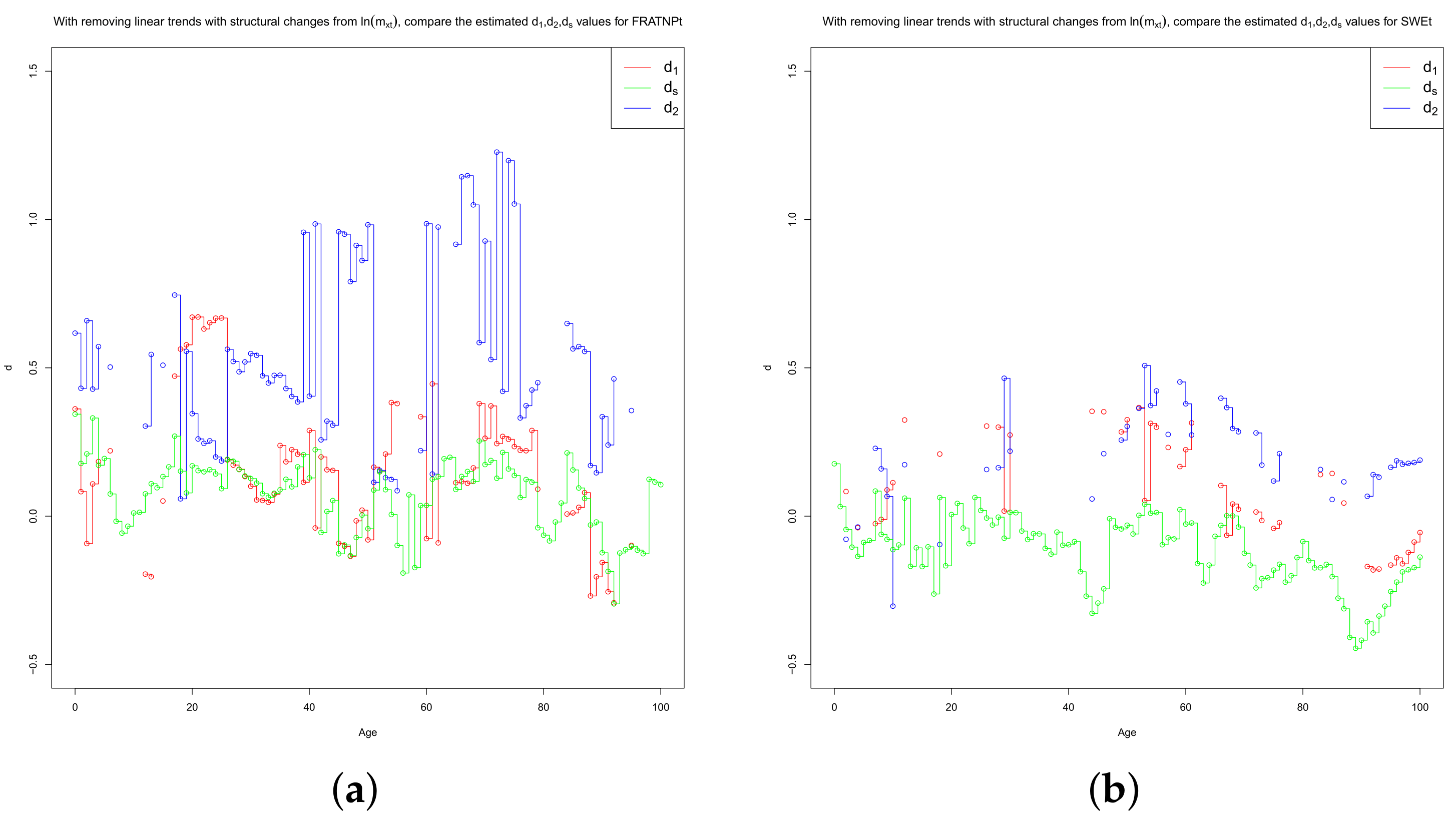
Furthermore, Figure 4 plots the fitted d 1 , d 2 and d s values for both countries’ mortality data. This figure shows that d s tends to underestimate in most cases. Especially for Sweden, d s is smaller than both d 1 and d 2 for almost all the ages, which means that d s underestimates the persistence for the whole period. This illustration is demonstrated also by simulation experiments in Section 3.3. Additionally, the d 1 and d 2 values are substantially different for most of the ages with observed structural change in d. Different values of persistence represent different features in time series, and the great change from d 1 to d 2 represents the important persistence feature change in mortality for the specific age, e.g., anti-persistent and stationary with short-memory ( d 1 = −0.0924) changed to mean-reverted nonstationarity ( d 2 = 0.6589) for age-2 of the France data. However, d s cannot capture such crucial dynamics in mortality since it doesn’t consider the structural change in persistence. These indicate that the MR test in our model considering structural change in d has a big advantage over the ordinary single persistence estimators not considering structural change. It is also demonstrated in Section 3.3 that: for a simulated time series with structural changes both in persistence and linear trend, after detrending it adequately, our model provides more accurate estimates of d 1 , d 2 than the estimated single d s .
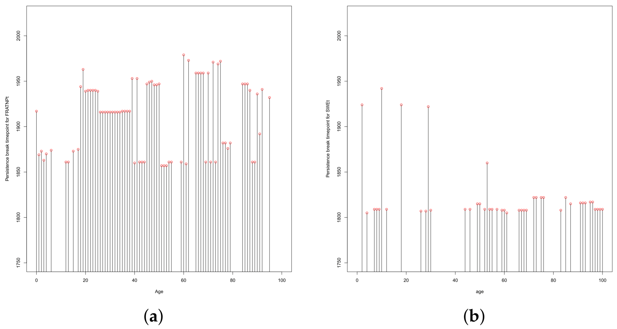
In addition, Figure 5 displays the fitted break timepoints in persistence for each age which has a structural change in persistence, for both France and Sweden l n ( m x t ) data detrended adequately. The estimated break timepoints in persistence for France total population mainly happen around 1860–1880, 1916–1917 (the World War I) or 1939–1959 (the World War II and thereafter). The break timepoints in persistence for Sweden mainly happened during 1805–1822, except a few in the 20th century. The early 19th century is an important period for Sweden when many big events happened, including participating in wars then adopting a neutrality and non-aligned foreign policy in 1814, and Sweden remained neutral in World War I and World War II. These indicate that wars might be a major factor that influences the persistence feature of a country’s total population. Earlier studies of Swedish mortality have also singled out the early nineteenth century as interesting, with one paper dividing Swedish mortality data into two periods with 1815 as the dividing point Bengtsson and Bröstrom (2011). Besides war, there are other possible factors that could explain a persistence break; for instance, penicillin was widely introduced in France by the allies at the end of World War II, which in some sense permanently changed people’s medical condition and might have contributed to the change in persistence. The papers Fu et al. (2022); Fu et al. (2025) observed mortality structural changes during the World War II and shortly thereafter. Also, Fu et al. (2025); Hainaut (2012) consider regime switching of mortality and both find that France population mortality is in a different state during the World War II and shortly thereafter. But these studies have not clarified whether the changes are in trend or persistence. For France total population, our approach observes that around the time of the World Wars, there were changes in persistence for ages 20–38 (Figure 1b), but changes in trend happen for a much wider age range, 1–80 (as will be seen later).
We have studied total country population because our main purpose is to demonstrate that persistence breaks occur. The question then arises about what happens when you study subpopulations, such as men and women separately. A detailed study could make interesting future work. But we did similar computations to those above, just for French males and French females seperately, and then for French civilians.
Some general observations: for women, the percentage of all ages found to have no break in persistence was somewhat higher (58.42% vs. that of men 73.27%), and the estimated d values for all ages tended to be somewhat lower. Visually in the heatmaps, there is a clear pattern in Figure 1b where from ages 20–25 and then from ages 26–38, a break is observed always observed around World War II and then around World War I, respectively. The same pattern is seen just looking at data for males, but the pattern is much less strong for civilian-only data and disappears for female data. Since almost all people directly in combat were male, this supports the notion that the breaks seen for the total population for ages 20–38 were very likely due to the World Wars.
Interestingly, a new strong pattern emerges for the civilian data: ages 31–50 all show a break around the same time in France during the late 1850s. (If we have to speculate, perhaps this was due to the terrible third cholera epidemic that hit France in 1854).

3.2. Structural Change in Persistence vs. Structural Changes in Linear Trend

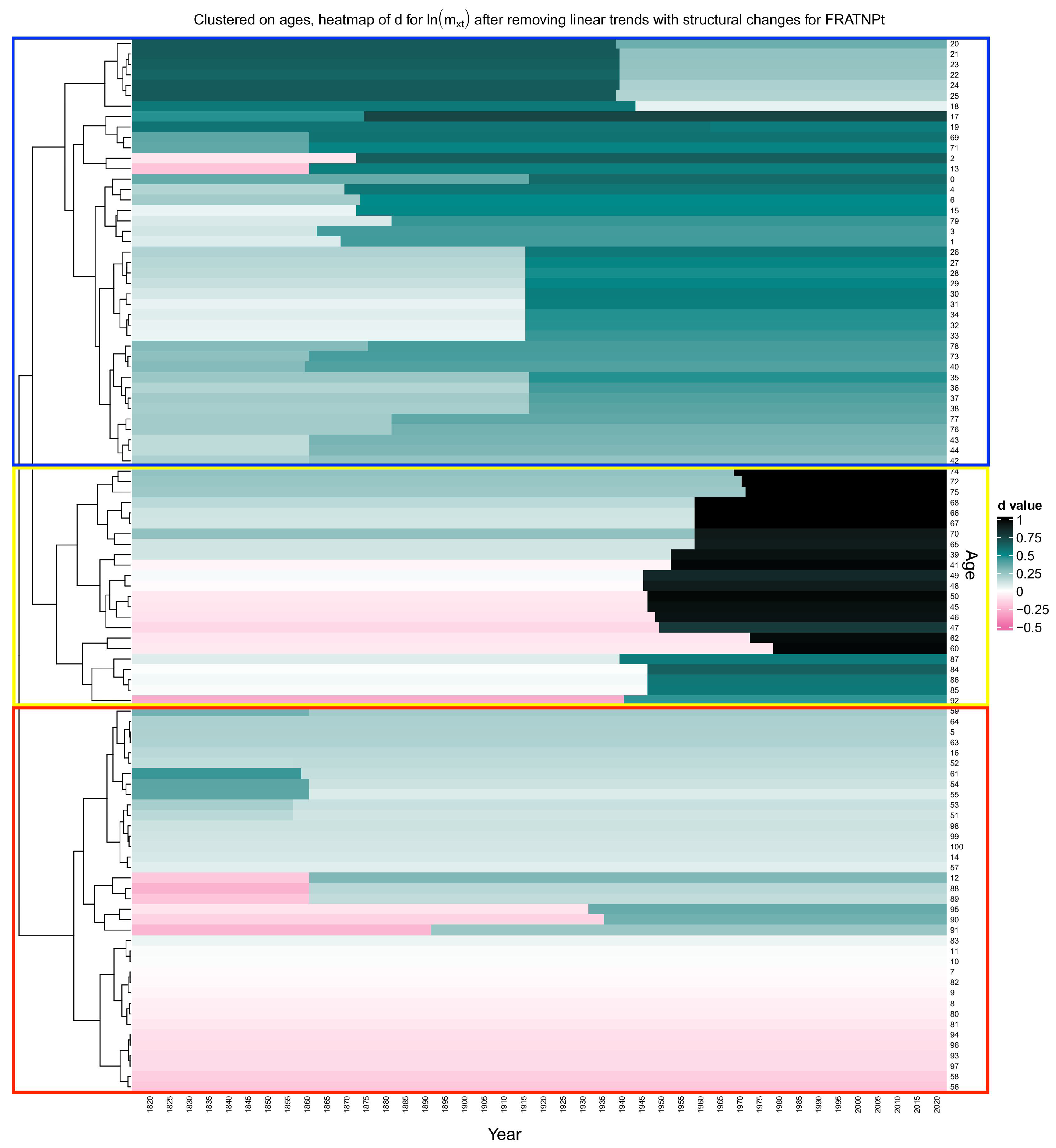
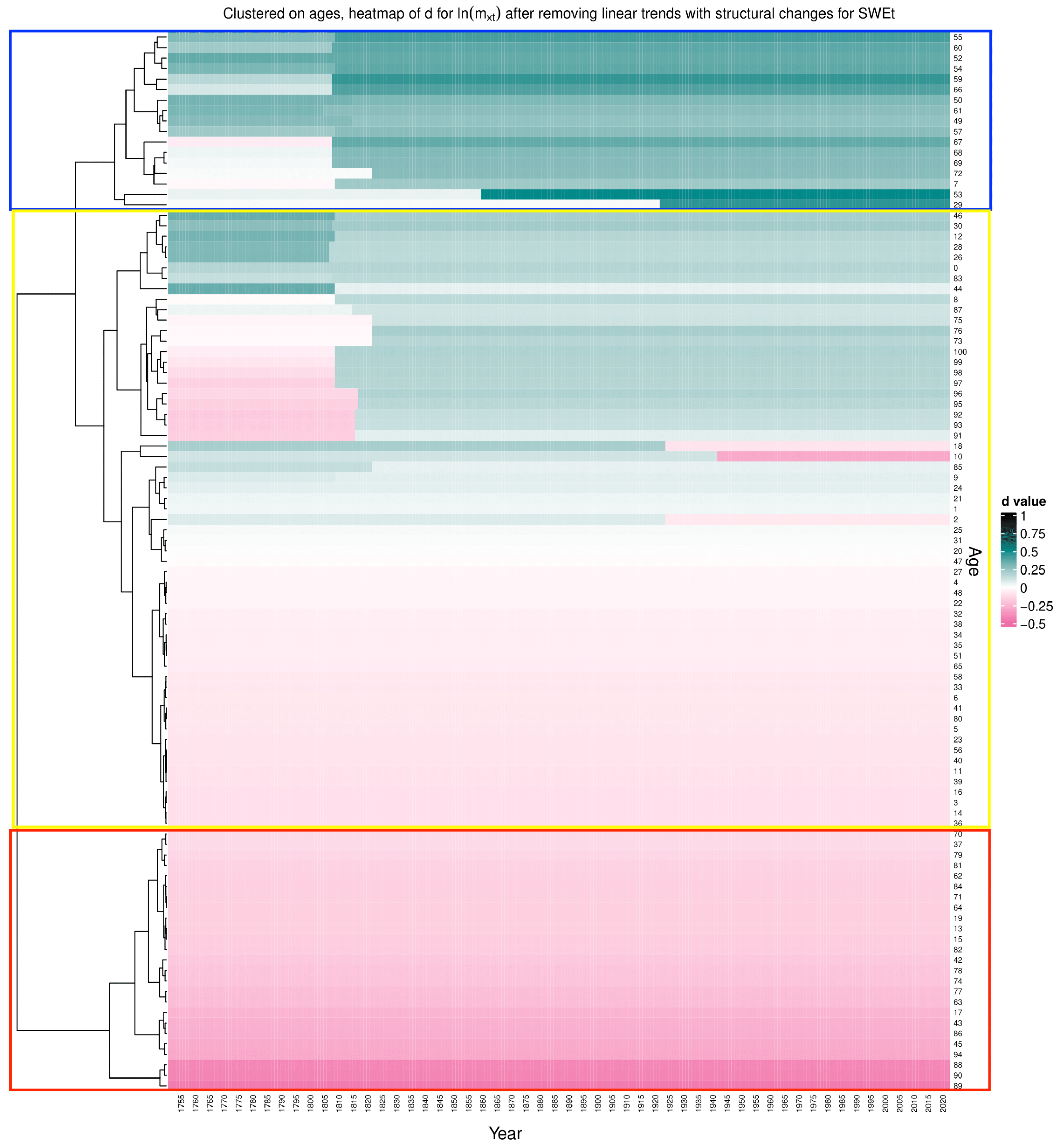
We are interested in the similarity of the structural changes in persistence among ages. So we performed a Hierarchical cluster analysis with the Euclidean distance as the measure of dissimilarity and the complete method to the d values (as a matrix of d value age by year) to cluster ages. We applied the function “Heatmap” in the R package ComplexHeatmap (Gu et al. (2016); Gu (2022)) to complete this task and create the corresponding heatmaps, shown in Figure 6 for France and Figure 7 for Sweden.
The clustering results imply three significant factors to determine the similarity of structural changes in persistence among ages in the clustering process: whether there is a structural change in persistence observed for this age or not; the amplitude of the change from d 1 and d 2 ; whether it is an increase or decrease from d 1 to d 2 . This might be a promising new age clustering method, which gives insightful information about mortality dynamics.
The persistence order measures the dissipating speed of the effect of an exogenous shock on the time series. For each age x, our approach models the logarithm of mortality l n ( m x t ) as the sum of its trend and a fractionally integrated process p t with order d t , as in Equation (4). If an exogenous shock with negative effect happens and causes a sudden increase in mortality, besides the possible increase in its trend, the shock may also boost p t suddenly and this is also a portion of the increase in mortality. The persistence order d t gives insightful information about whether this increase in p t is transient or permanent, and if it is transient, how long will it last. This will affect the mortality risk in some following time period and so provides useful information for possible health policy invention.
In Figure 6, we see a group of ages in the middle part of the figure presents very high d 2 values in the recent half century, close to or even bigger than 1, meaning very long-term or even permanent effects of disturbances. For France, this group of ages tend to be more “vulnerable” to recent harmful exogenous shocks and may need special attention. A recent shock that only has a very short-term effect on p t for another group of ages (like the bottom ones with anti-persistent d < 0 in this figure), may cause a permanent increase in p t for this “vulnerable” age group. Clustering age according to persistence may benefit mortality risk analysis and health policy choosing.
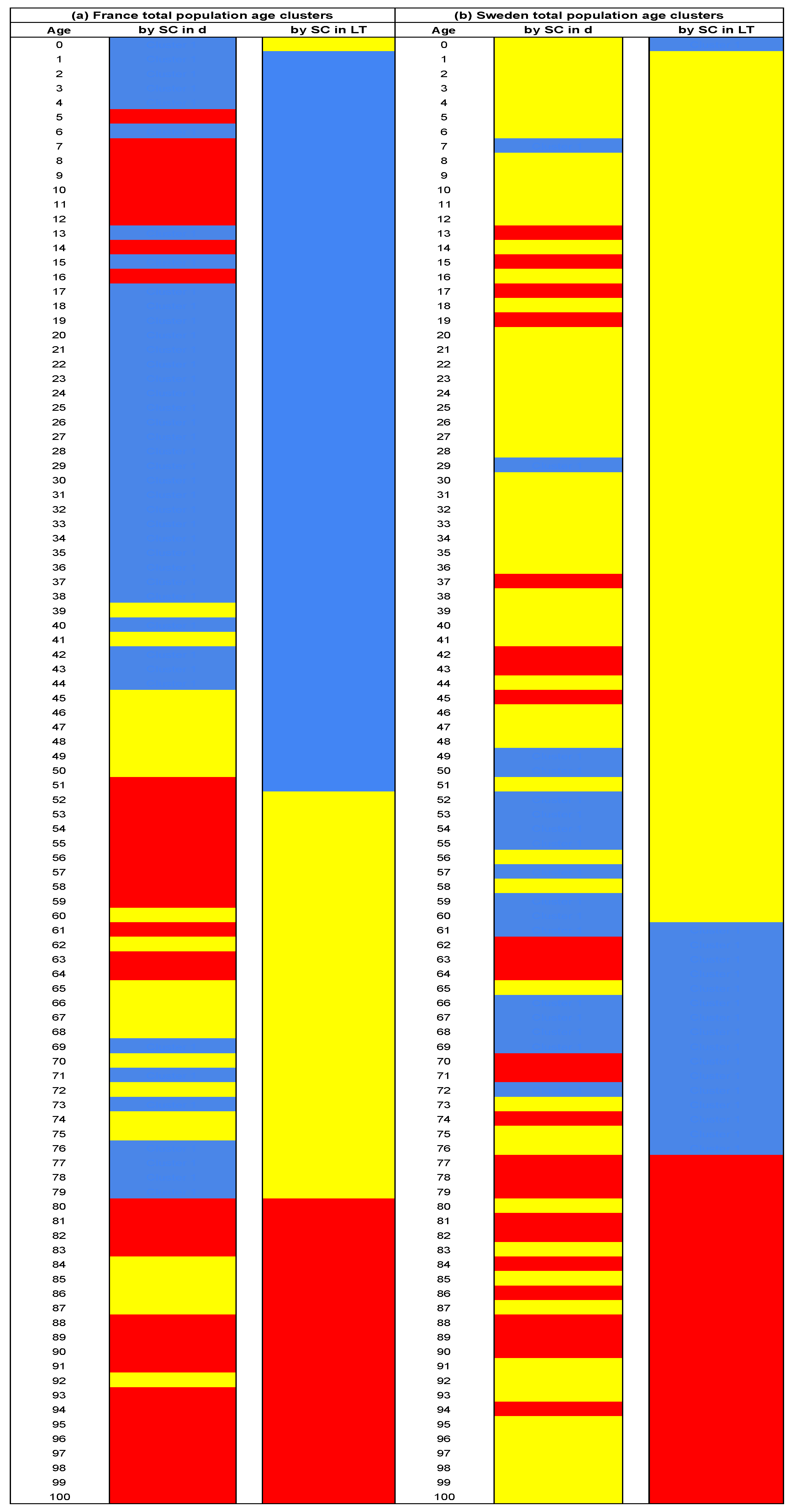
Taking the 3-cluster case as an example, Figure 8 displays the three age clusters using different colors, which are also marked by corresponding color boxes in Figure 6 and Figure 7. The second column and the fifth column are the results from clustering based on the structural change in persistence for France and Sweden respectively. The three clusters for France, cluster yellow and cluster blue for Sweden all present an age consecutive pattern to some degree. One can observe that the majority of young ages and early adulthood (ages 0–44) are in the same cluster for both countries, which means that these ages share similar features in persistence. However, older adulthood and old-age experience more complicated dynamics in persistence features and don’t show age consecutive clusters.
We also performed a similar Hierarchical cluster analysis to the removed linear trend with structural changes in l n ( m x t ) , in order to compare the structural change in persistence and the structural changes in linear trend, and the resulting 3 age clusters are displayed in Figure 8 column 3 (for France) and column 6 (for Sweden). We can see that if the ages are clustered based on the linear trend with structural changes, except for age 0, all three clusters show a strong age consecutive pattern for both countries. For example, column 6 implies that young ages (not including infant age) till adulthood (1–60), age 0 & early old ages (0, 61–76) and later old ages (77–100) are three age clusters. For the linear trend with changes, they share similar features inside the clusters but present different features outside the clusters.
When comparing the clustering results from the change in persistence and the changes in linear trend, we see that the structural changes in linear trend show a much stronger age consecutive pattern than the structural change in persistence. Moreover, a specific age may have very different persistence features and trend features. For instance, age 0 of the France total population has similar persistence features as the young ages and early adulthood (Cluster Blue of column 2), while has different features in its trend, not like the young ages and early adulthood (Cluster Blue of column 3) but like the older adulthood and early old ages (Cluster Yellow of column 3). Furthermore, by comparing the break timepoints for changes in persistence and for changes in linear trend, again a much stronger age consecutive pattern is observed in the latter than the former, which is both true for France and Sweden. Here we only provide the heatmap of the removed linear trend with changes for France data in Figure 9 as evidence and by comparing the breakpoints in Figure 1b and Figure 9 one can draw a similar conclusion.
Comparison of Figure 1b and Figure 9 demonstrates the statement in the introduction that the timing and direction of a change in persistence is not intuitive, as it is with the trend. For instance, a break in mortality dynamics is to be expected when France was involved in a World War. In Figure 9, every age from 1 to 80 except for age 19 shows a break in trend during the period 1940–1946, when France was heavily involved in World War II or just after. Figure 1b shows much more variety in timing and direction of breaks in persistence. The breaks for people of fighting age, from 20 to late 30s, are during World War I or World War II. But the direction of the change—whether persistence increases or decreases at the time of the war—is not always the same. And most other ages not in this range (so the majority of ages) experience persistence breaks at times not during or shortly after the world wars or else do not experience a persistence break at all. For instance, many ages across the spectrum of all ages either experience no break or a break around the 1860s–1870s in persistence, as shown in Figure 5. None of the possible three breaks in trend seen for these ages happened at that time. On the other hand, the strong break in trend observed for all of these ages around World War II is not reflected in the heatmap for persistence. So exogenous shocks intuitively thought to strongly influence the mortality usually affect the trend but not necessarily the persistence, and conversely, there are some factors affecting persistence while not affecting the trend. Concerning the breaks in French mortality persistence in the nineteenth century (1860s–1870s): earlier studies have found significant features in French mortality data around mid-1800s, for instance Preston and van de Walle (1978), which suggests that improvements in sewerage and drinking water systems starting in the 1850s drove mortality changes. Thinking of persistence as responsiveness of mortality data to shocks, it makes sense that long-term improvements to public health would affect the ability of disease to spread, etc., which would correspond to a change in persistence. For Sweden, the fitted piecewise linear trend shows a break near 1918 for ages 12–43, confirming a structural break in mortality trend obtained by a different method by Lundström and Qvist (2004) in 1918 when considering Sweden data across ages 10–99 together. Moving from purely statistical observations to the demographic context, Sweden was neutral in World War I, so they identify this as probably due to the Spanish Flu epidemic at the time. On the other hand, Figure 2 shows no break in persistence at this time for almost all ages, with the exception of age 18 and age 29).
All the differences observed between persistence dynamics and trend features above support an important idea in our model design: the dynamics of persistence and of trend are very different, and we need a careful method to consider them separately. We first model the trend features of l n ( m x t ) by a piecewise linear trend with structural changes, and then analyze its change in persistence by applying MR test to the adequately detrended l n ( m x t ) .
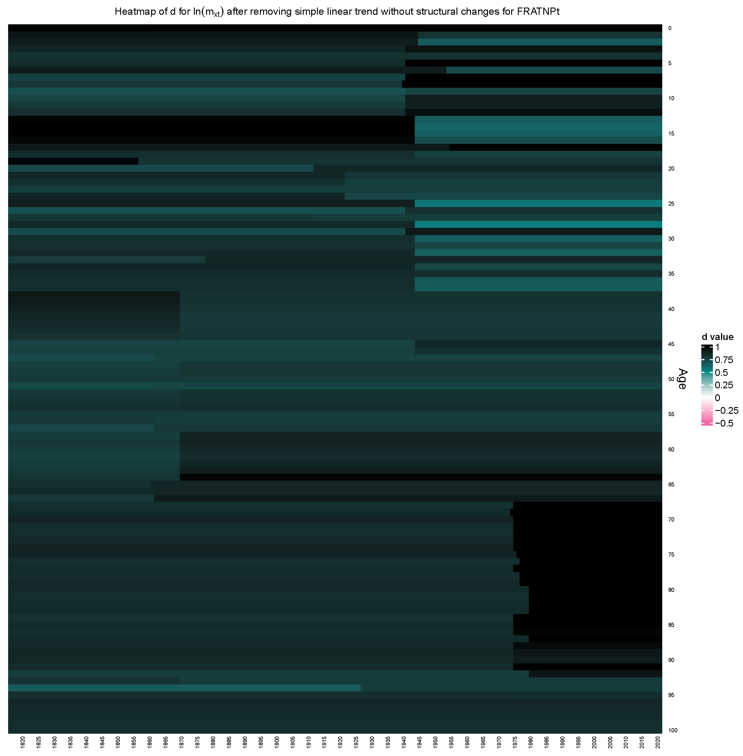
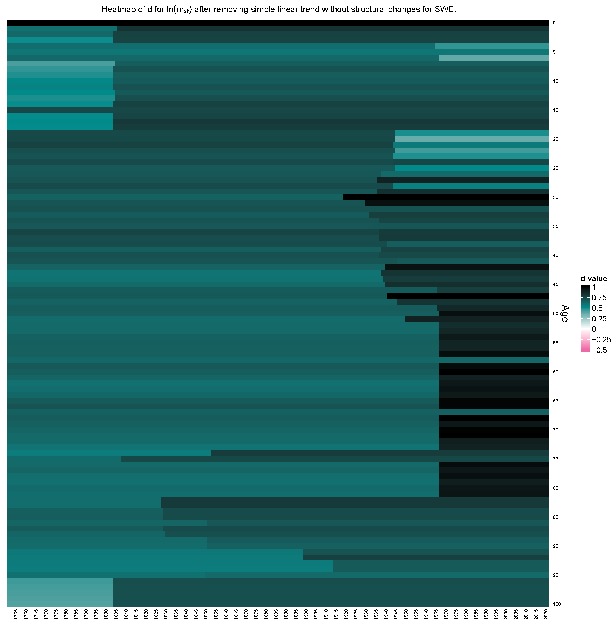
Considering structural changes in the linear trend of l n ( m x t ) is necessary in the detrending process and benefits the following estimation of persistence change. We compared our model results with the results obtained from a similar control experiment, which detrends l n ( m x t ) by removing the simple linear trend without considering structural changes in the trend and keeps other steps the same. Figure 10 and Figure 11 provide the heatmaps of d resulting from the control experiment for France and Sweden respectively. By comparing Figure 10 with Figure 1b and Figure 11 with Figure 2b, one can notice that without considering the structural changes in linear trend in the detrending progress, the persistence will be overestimated greatly, indicated by the much darker color in Figure 10 and Figure 11. Moreover, in the control experiments, there are 94.06% ages for France and 96.04% ages for Sweden among ages 0 to 100 which have an observed structural change in persistence at some timepoint. Recalling the percentages in our model results are 76.24% for France and 43.56% for Sweden. We conclude that the not-adequately-removed structural changes in linear trend of l n ( m x t ) may distort the following estimation of persistence change, even wrongly draw the deduction that almost all the ages experience structural change in persistence.

3.3. Accuracy of Persistence Estimation by Testing on Simulated Data

Because there is not any direct measure about persistence that can be observed from mortality data directly, we test our model on simulated time series data in order to analyze the accuracy with which it reproduces the value of the persistence, compared with two control models.
We simulated various time series data that have different length N, different persistence features and different trend dynamics. N, the length of the simulated time series is either 207 (equal to the period length of France total population data) or 272 (equal to the period length of Sweden total population data). For persistence features, we considered both cases with no change in persistence as well as cases with a change in persistence. For no-change in persistence cases, we tried 0.2 , 0.1 , 0.2 , 0.3 , 0.4 , 0.5 , 0.8 as the d s values for the whole period of time series. For cases with a change in persistence, we tried ( 0.1 , 0.4 ) , ( 0.2 , 0.4 ) , ( 0.2 , 0.6 ) , ( 0.2 , 0.8 ) , ( 0.2 , 1.2 ) , ( 0.4 , 0.8 ) , ( 0.2 , 0.3 ) , ( 0.1 , 0.7 ) , ( 0.1 , 0.9 ) , ( 0.4 , 0.1 ) , ( 0.6 , 0.2 ) , ( 0.2 , 0.2 ) as ( d 1 , d 2 ) values. And in cases with a change in persistence, we also assumed different break timepoints T d happening near the beginning, middle and the end of the time series by setting it to be the integer closest to the 25th, 50th and 75th quantile of 1 , 2 , , N respectively. We assumed the trend dynamics as a piecewise linear function in our data simulation, and we directly used the fitted linear trend with structural changes for age {0,20,85} of France or Sweden mortality data from our model results in Section 3.1 as different trend dynamics. If N = 207 , we use the fitted linear trend with structural changes determined from the France data; if N = 272 , we use that from the Sweden data.
As for the data simulation process, we first simulate a length-N fractional white noise process (as in Equation (A3)) with chosen persistence features, including assumptions about existence of a change, d s or ( d 1 , d 2 ) values and breakpoint. Then we add the assumed trend dynamics (as a piecewise linear function) to the fractional white noise process to obtain the time series as one simulated data. The creation of the fractional white noise process has randomness, so for each set of assumptions, we repeat the above process 1000 times to generate 1000 time series. The set of assumptions refers to the length of the time series N, whether there exists a break in persistence, assumed d s or ( d 1 , d 2 ) values, the assumed break time point if it exists, and the assumed piecewise liner trend. Our simulated data comprised 258,000 time series presenting 258 different assumption setups in total, and we tested our model and two control models on each time series in the simulated data. Below are the descriptions of the three models and some notations:
  • Our model, denoted as M, described in the Section Check for Change in Persistence on Detrended Mortality Data;
  • Control model 1, denoted as M1: it has the same detrending process as M but doesn’t consider structural change in persistence, instead it provides the single persistence d s . M 1 for the whole period by applying the Gaussian Semiparametric local Whittle estimator to the adequately detrended time series;
  • Control model 2, denoted as M2: it detrends ln(mxt) by removing the simple linear trend without considering structural changes in trend, and then provides the single persistence d s . M 2 for the whole period by applying the Gaussian Semiparametric local Whittle estimator to the detrended time series.
For each assumption setup and the associated 1000 time series, we record the following items as the testing results of the three models:
  • For M:
    the percentage of time series with an observed change in persistence among the 1000 time series, denoted as % ( d S C ) ;
    m ( d 1 ^ ) d 1 for those time series with an observed change in persistence, where d 1 ^ denotes the estimated d 1 for a single time series and m ( d 1 ^ ) denotes the mean of all fitted d 1 ^ s;6
    m ( d 2 ^ ) d 2 for those time series with an observed change in persistence, where d 2 ^ denotes the estimated d 2 for a single time series and m ( d 2 ^ ) denotes the mean of all fitted d 2 ^ s.
  • For M1:
    m ( d s ^ . M 1 ) d 1 and m ( d s ^ . M 1 ) d 2 if a break in persistence is assumed, where d s ^ . M 1 denotes the estimated d s . M 1 for a single time series and m ( d s ^ . M 1 ) denotes the mean of all fitted d s ^ . M 1 s;
    m ( d s ^ . M 1 ) d s if no break in persistence is assumed.
  • For M2:
    m ( d s ^ . M 2 ) d 1 and m ( d s ^ . M 2 ) d 2 if a break in persistence is assumed, where d s ^ . M 2 denotes the estimated d s . M 2 for a single time series and m ( d s ^ . M 2 ) denotes the mean of all fitted d s ^ . M 2 ;
    m ( d s ^ . M 2 ) d s if no break in persistence is assumed.
Table 1 reports the testing results of M, M1, M2 on the simulated data. We consider two general cases of the simulated data: (a) time series assumed to have a structural change in persistence and (b) time series assumed to have no change in persistence. Case (a) includes 216 different assumption setups and 216,000 time series; Case (b) includes 42 different assumption setups and 42,000 time series. Column 1 and column 2 record the results for case (a); column 3 and column 4 record the results for case (b). Each number in column 2 and column 4 presents the mean value of the associated item (identified just to its left) for all the experiments considered. Taking −0.0436 as an example, after applying M on all the simulated time series in case (a), the mean of the error in d 1 ^ is −0.0436 for the 216,000 time series.
Model M provides the highest accuracy in the estimation of persistence among the three models. For the 216,000 case (a) time series assuming a change in persistence, model M recognizes the break existence for 67.19% of them and gives the lowest error in the estimation of d 1 and also in the estimation of d 2 , compared with M1 and M2. For instance, model M’s average error in estimating d 1 ^ is −0.0436; model M2 does not allow a break in persistence, and the average deviation of d s ^ . M 2 from d 1 is many times larger, at 0.7052. For the 42,000 case (b) time series assuming no change in persistence, M claims no change in persistence correctly for 1 − 33.40% = 66.60% of them. For the 33.40% series claimed by M wrongly to have a break in persistence, M still gives estimated d 1 ^ and d 2 ^ with much less error (−0.1609 and −0.0826) than the estimated d s ^ . M 1 from M1 (−0.3263, more than twice of the bigger error of Model M) and the estimated d s ^ . M 2 from M2 (0.5649, about 3.5 times of the bigger error of Model M), even though those proceed with the correct assumption that there is no break in persistence. Also, the difference 0.1609 ( 0.0826 ) = 0.0783 shows that even though model M wrongly thinks there was a change in persistence, it also decides that the change is very small. We used a significance level of 10%, and if decreased, the proportion %(dSC) would improve.
Moreover, one can notice that M1 tends to underestimate persistence greatly for both case (a) and case (b) simulated data. This matches the assertion we made in Section 3.1 resulting from comparing the part (a) and part (b) of Figure 1 and Figure 2: for adequately detrended l n ( m x t ) , estimated single persistence d s without considering the structural change in d always underestimates the real persistence feature.
M2 tends to overestimate persistence greatly for both case (a) and case (b), which results from the not-adequately-removed structural changes in linear trend of the time series. This is an example of the overestimation that can sometimes produce what is called “spurious long memory.” A simple linear regression without considering the structural changes in the linear trend is not enough to detrend the time series. This supports our conclusion in Section 3.1 that the not-adequately-removed structural changes in linear trend will distort the following persistence estimation. (Also possible is something that maybe be described as “over-detrending”, leading to underestimation of true persistence. If a complex process is used to model trend, it can mistakenly capture what is actually persistence as detail in the trend, thereby misrepresenting the remaining persistence when the deterministic process is removed. See, for instance, Granger and Hyung (2004)).
We used the control variates method to analyze how the factors of N, T d and d 2 d 1 affect the model M results on the simulated data. We found that when d 2 d 1 is positive and increases, %(dSC) shows a clear increasing trend. %(dSC) is 17.51%, 27.56%, 66.13%, 72.90%, 86.81%, 92.57% and 97.75% for d 2 d 1 = 0.2, 0.3, 0.4, 0.5, 0.6, 0.8, 1.0 respectively. For the cases where persistence increases, a greater increase in persistence will help our model to recognize the change, but the results don’t show the same benefit to the accuracy of persistence estimation. Furthermore, the change of T d and N has not shown great influence on the results.

4. Conclusions

In recent decades, mortality literature captured the long memory generally existing in mortality data, which helps researchers to better understand the mortality dynamics and improves mortality models’ fitting and forecasting. However, the possible change in persistence degree in mortality data has never been considered.
Our paper the first time considers the structural change in persistence of mortality, and also, it is the first time that the powerful MR test Martins and Rodrigues (2014) used in macroeconomics is applied to mortality time series. We find that a significant portion of the full ages have experienced structural change in the persistence of mortality. For example, 76.24% ages for France total population and 43.56% ages for Sweden total population among ages 0 to 100 are observed to experience a change in persistence of mortality (after adequately detrending its logarithm).
In Section 3.1, we provide the heatmaps of fitted persistence degrees for each year and each age. One can observe important persistence feature changes in the heatmaps: from stationary long-memory to nonstationarity, from anti-persistence to long-memory, from anti-persistence to nonstationarity, etc. Depending on different persistence features of the mortality, sudden exogenous shock will have a different effect, like a temporary effect on stationary series, but a permanent effect on not-mean-reverted, nonstationary series. So the change in persistence degree of mortality series should not be neglected.
Moreover, our approach is the first study to consider the structural change in persistence as well as the structural changes in trend of mortality both and separately, and compare their difference. Persistence estimation is easily confused and distorted by the structural change in trend of the time series. Before we apply the MR test to detect the structural change in persistence and estimate the persistence, we detrended the mortality series by removing its trend with structural changes and verified that the detrending process is adequate by testing the mean change under long memory on the detrended series. By comparing the age clustering based on the two types of structural change and also their fitted break time points, we conclude that the two types of structural change are very different. Especially, the structural changes of trend show a much stronger age consecutive pattern compared to the structural changes in persistence.
Furthermore, we test our model on simulated data and compare it with two other control models that do not consider the structural change in persistence, in order to analyze how well our model estimates the persistence. From the results, our model has the highest accuracy for the estimation of persistence among the three models.
There are several avenues for future work to extend this initial study of persistence change in mortality:
  • Moving to other statistical models.
  • Studying the implications for forecasting.
  • Turning to other populations and do explanation in demographic context.
For 1, We study age-specific mortality series using the standard Lee-Carter model because this is a first investigation of structural change in persistence in mortality. But certainly we could turn in the future to a standard extension of Lee-Carter, for instance one including a cohort effect, or even to other types of models (surveyed, for instance, in Macdonald et al. (2018)).
We model the structural changes in trend of mortality by a piecewise linear trend for simplicity, and all the detrended series show no significant change in mean under long memory, meeting our needs. However, the logarithm of mortality series for some single ages may have nonlinear trend and fitting it by a piecewise linear function may not be enough. In the future, to refine our model, we may further consider nonlinearity with structural changes of the trend and the change in the persistence in our mortality model. This would be delicate and should be done carefully though, because it is known that "overdetrending" is an issue, whereby persistence in a time series can be captured as part of the trend, so that after the trend is removed, the fitted persistence of the residuals is biased to be too low. This is demonstrated, for instance, by Granger and Hyung (2004).
For 2, forecasts of mortality inform actuarial practice, like pricing, as well as broader governmental policy. The present article shows that it is warranted to perform detailed study of how, when using fractional ARIMA models, the forecast accuracy improves when accounting for breaks in persistence.
And for 3, the present work highlights some differences when studying France and Sweden. Demographic factors certainly can account for some differences: for instance, France was involved in World War I, while Sweden was neutral. But other differences are more mysterious. For instance, France tends to show a larger jump in persistence when the MR test detects a break, compared with the jump for Sweden. We studied just two countries in this first investigation partly because we found looking at a couple of additional countries that they had some similarity to France or Sweden; for instance, England gives results more similar to France in most respects than to Sweden. To keep things simple, we stick with two countries that demonstrate that the present observations about persistence are country-specific, highlighting two countries with a good contrast.
There are certainly other explanations for persistence breaks and values than we provide that may be illuminated by further study. And we provide no explanations for how, intuitively, one might expect a jump upward versus downward in persistence when a break is detected. Understanding the contexts in which a break in persistence may be expected, and the nature of that break, could add a useful complement to forecasting when setting policy or making actuarial decisions.

Author Contributions

Conceptualization: W.F. and B.R.S.; methodology: W.F. and B.R.S.; software: W.F.; validation: W.F. and B.R.S.; formal analysis: W.F.; investigation: W.F.; resources: Publicly available data from Human Mortality Database (HMD); data curation: HMD data is ready-to-use; writing—original draft preparation: W.F.; writing—review and editing: W.F., B.R.S. and P.B.; supervision: W.F.; project administration: W.F. and B.R.S.; visualization: W.F.; funding acquisition: W.F and B.R.S. All authors have read and agreed to the published version of the manuscript.

Funding

The APC is covered by the 2025–26 research and professional development grant funded by Lebanon Valley College. The grant has no grant number.

Institutional Review Board Statement

Not applicable.

Informed Consent Statement

Not applicable.

Data Availability Statement

Data available in a publicly accessible repository that does not issue DOIs. Publicly available datasets were analyzed in this study. This data can be found here: Human Mortality Database. University of California, Berkeley (USA), and Max Planck Institute for Demographic Research (Germany). Available at www.mortality.org or www.humanmortality.de (data downloaded on 10 June 2025).

Conflicts of Interest

The authors declare no conflict of interest.

Appendix A

Testing Structural Change in Persistence Parameter d by the MR Test

The MR test is capable of detecting changes between fractionally integrated processes with different persistence parameter d. The MR test is based on the recursive forward and reverse estimation of the Breitung and Hassler (2002) test.
Given a time series { z t } t = 1 , 2 , , T , the Breitung and Hassler (2002) test tests the hypothesis that the studied { z t } is an I ( d ) process satisfying ( 1 L ) d z t = ϵ t , where ϵ t is white noise with mean zero and constant variance. Defining Z t ( 1 L ) d z t , the test is equivalent to test the hypothesis that Z t is white noise against that Z t I ( θ ) with some θ 0 .
Under the assumptions of z t = 0 , t 0 and independent and identically distributed (i.i.d.) ϵ t N o r m a l ( 0 , σ 2 ) , they consider the regression
Z t = α Z t 1 + e t , where Z t 1 = Σ j = 1 t 1 j 1 Z t j
and derive the score statistic as the squared t-statistic for α = 0 :
Ω T 2 = ( Σ t = 2 T Z t Z t 1 ) 2 σ e 2 ^ Σ t = 2 T Z t 1 2 ,
where σ e 2 ^ is the usual regression estimate for the variance of e t . Breitung and Hassler (2002) demonstrate that under the null hypothesis, the statistics Ω T 2 d χ 2 ( 1 ) as T .
The MR test considers an A R I M A ( 0 , d t , 0 ) process { y t } t = 1 , 2 , , T satisfying
( 1 L ) d t y t = ϵ t
where y t 0 for t 0 and ϵ t is i.i.d. white noise. Its null hypothesis assumes that d t is constant over the sample, i.e., d t = d s . However under the alternative, a structural change in persistence takes place at time [ τ T ] with unknown τ in [ Λ l , 1 Λ l ] [ 0 , 1 ] , and d t changes its value from d 1 in the first regime to d 2 in the second regime. Λ l is pre-determined (typically 0.15 or 0.20 in literature) and the alternative considers two cases: (1) a decrease in persistence d 1 > d 2 and (2) an increase in persistence d 1 < d 2 .
The MR test follows Breitung and Hassler (2002) and derives several statistics similarly. Under the null hypothesis d t = d s , let Y t = ( 1 L ) d t y t and consider the auxiliary regression for each fixed τ [ Λ l , 1 Λ l ] :
Y t = α ( τ ) Y t 1 + v t , t = 2 , 3 , [ τ T ] , where Y t 1 = Σ j = 1 t 1 j 1 Y t j
Then the forward statistic is derived as the infimum of the t-statistic associated with α ( τ ) as τ move recursively. Denoting the t-statistic associated with α ^ ( τ ) = 0 as t α f ( τ ) and the forward statistics as Ω f , then we have
t α f ( τ ) = Σ t = 2 [ τ T ] Y t Y t 1 σ ^ v ( τ ) Σ t = 2 [ τ T ] Y t 1 2 , and Ω f inf τ [ Λ l , 1 Λ l ] t α f ( τ ) ,
where σ ^ v ( τ ) is the usual regression estimate for the standard deviation of v t in (A4).
Similarly a reverse statistic Ω r can be derived by considering the time-reversed series V t Y T t + 1 and the corresponding auxiliary regression for each τ :
V t = α ( τ ) V t 1 + u t , t = 2 , 3 , [ ( 1 τ ) T ] , where V t 1 = Σ j = 1 t 1 j 1 V t j .
We have
t α r ( τ ) = Σ t = 2 [ ( 1 τ ) T ] V t V t 1 σ ^ u ( τ ) Σ t = 2 [ ( 1 τ ) T ] V t 1 2 , and Ω r inf τ [ Λ l , 1 Λ l ] t α r ( τ ) ,
where σ ^ u ( τ ) is the usual regression estimate for the standard deviation of u t in (A6).
We also provide a schematic diagram for the steps to derive the MR test statistics Ω f and Ω r in Figure A1.
Furthermore, if the direction of change in persistence is unknown under the alternative, as is generally the case, the statistic Ω m i n = m i n { Ω f , Ω r } is recommended.
Martins and Rodrigues (2014) demonstrate the following limit null distributions: as T ,
  • for any fixed, known τ [ Λ l , 1 Λ l ] , both t α f ( τ ) and t α r ( τ ) d N ( 0 , 1 ) ;
  • Ω f inf τ [ Λ l , 1 Λ l ] W ( τ ) τ and W ( · ) represents a Wiener process;
  • Ω r inf τ [ Λ l , 1 Λ l ] W ( 1 ) W ( τ ) 1 τ ;
  • Ω m i n min inf τ [ Λ l , 1 Λ l ] W ( τ ) τ , inf τ [ Λ l , 1 Λ l ] W ( 1 ) W ( τ ) 1 τ
They also state that Ω r has better performance for the case of d 1 > d 2 and Ω f has better performance for the case of d 1 < d 2 based on theoretical results. Equivalently, the squares of the t-statistics in (A5) and (A7) can be also considered, and their supremum and the maximum of the two suprema can be a another set of statistics for the MR test.
Breitung and Hassler (2002); Martins and Rodrigues (2014) also mention that the time series Z t and Y t can be demeaned or detrended prior to computing the statistics, which doesn’t affect the limiting distributions. Additionally, both papers consider the persistence or persistence change for an A R I M A ( p , d , 0 ) process. That says ϵ t = ( 1 L ) d z t or ( 1 L ) d t y t is a stable A R ( p ) . But it is out of our scope and we omit it for brevity.
Figure A1. Schematic diagram about deriving statistics Ω f and Ω r in the MR test.
Risks 13 00225 g0a1

Notes

1
Our approach follows the use of the range of d as ( 0.5 , 2 ) in the MRtest function in R package memochange.
2
A stationary process is said to have long memory if its autocovariance γ j for lag j satisfies lim T Σ j = T T | γ j | = .
3
The series p t and the order d t actually depend on the age x, as does the number of breaks b and the breakpoints T 1 , , T b discussed in the following point 2. We will only use this notation in a context where the age is fixed, so for simplicity we exclude the age from these notations.
4
While long time series are preferable to study long memory behavior, it should be noted that both countries have decreased quality of mortality data once you get back into the nineteenth century, for various reasons. See the files on background and documentation for Sweden and France on the HMD website.
5
If we change the rejection threshold from 10% to 5% to 1%, the percentage for France does not drop much (from 76.24% to 69.31% to 60.40%), but the percentage for Sweden drops substantially (from 43.56% to 24.75% to 6.93%). This probably reflects the observation that the change in fitted d values at a break tends to be larger for each age of the France data than when compared to the changes in d for the Sweden data. Since we do not know for a case removed upon dropping the significance level whether that was because it was a false positive or because it was a true positive with a modest effect, and since we do not want to miss breaks in persistence and consider the good accuracy of our model even for false break claiming, we use 10% for the remainder of the paper.
6
If no break in persistence is assumed for the simulation of a time series but M observed change in persistence in it, m ( d 1 ^ ) d 1 will be m ( d 1 ^ ) d s and m ( d 2 ^ ) d 2 will be m ( d 2 ^ ) d s .

References

  1. Bengtsson, Tommy, and Göran Bröstrom. 2011. Famines and mortality crises in 18th to 19th century southern Sweden. Genus 67: 119–39. [Google Scholar]
  2. Ben Nasr, Adnen, Ahdi Noomen Ajmi, and Rangan Gupta. 2014. Modelling the volatility of the Dow Jones Islamic Market World Index using a fractionally integrated time-varying GARCH (FITVGARCH) model. Applied Financial Economics 24: 993–1004. [Google Scholar] [CrossRef]
  3. Bishai, David M. 1995. Infant mortality time series are random walks with drift: Are they cointegrated with socioeconomic variables? Health Economics 4: 157–67. [Google Scholar] [CrossRef]
  4. Box, George E. P., and Gwilym M. Jenkins. 1976. Time Series Analysis Forecasting and Control, 2nd ed. San Francisco: Holden-Day. [Google Scholar]
  5. Breitung, Jorg, and Uwe Hassler. 2002. Inference on the cointegration rank in fractionally integrated processes. Journal of Econometrics 110: 167–85. [Google Scholar] [CrossRef]
  6. Busetti, Fabio, and A. M. Robert Taylor. 2004. Tests of stationarity against a change in persistence. Journal of Econometrics 123: 33–66. [Google Scholar] [CrossRef]
  7. Caporale, Guglielmo Maria, and Luis A. Gil-Alana. 2014. Infant mortality rates: Time trends and fractional integration. Journal of Applied Statistics 42: 589–602. [Google Scholar] [CrossRef]
  8. Cheung, Yin-Wong. 1993. Tests for Fractional Integration: A Monte Carlo Investigation. Journal of Time Series Analysis 14: 331–45. [Google Scholar] [CrossRef]
  9. Davidson, James, and Andrea Monticini. 2010. Tests for cointegration with structural breaks based on subsamples. Computational Statistics & Data Analysis 54: 2498–511. [Google Scholar] [CrossRef]
  10. Diebold, Francis X., and Atsushi Inoue. 2001. Long memory and regime switching. Journal of Econometrics 105: 131–59. [Google Scholar] [CrossRef]
  11. Diebold, Francis X., and Glenn D. Rudebusch. 1991. On the power of Dickey-Fuller tests against fractional alternatives. Economics Letters 35: 155–60. [Google Scholar] [CrossRef]
  12. Dreger, Christian, and Hans-Eggert Reimers. 2005. Health Care Expenditures in OECD Countries: A Panel Unit Root and Cointegration Analysis. International Journal of Applied Econometrics and Quantitative Studies, Euro-American Association of Economic Development 2: 5–20. [Google Scholar] [CrossRef]
  13. Fu, Wanying, Barry R. Smith, Patrick Brewer, and Sean Droms. 2022. A New Mortality Framework to Identify Trends and Structural Changes in Mortality Improvement and Its Application in Forecasting. Risks 10: 161. [Google Scholar] [CrossRef]
  14. Fu, Wanying, Barry R. Smith, Patrick Brewer, and Sean Droms. 2023. Markov-Switching Bayesian Vector Autoregression Model in Mortality Forecasting. Risks 11: 152. [Google Scholar] [CrossRef]
  15. Fu, Wanying, Sean Droms, Patrick Brewer, and Barry R. Smith. 2025. Applying Markov-switching Bayesian vector autoregression to an age-partitioned Lee–Carter mortality model. European Actuarial Journal 15: 417–43. [Google Scholar] [CrossRef]
  16. Gil-Alana, Luis A., Juncal Cunado, and Rangan Gupta. 2017. Persistence, Mean-Reversion and Non-linearities in Infant Mortality Rates. Soc Indic Res 131: 393–405. [Google Scholar] [CrossRef]
  17. Granger, Clive W. J., and Namwon Hyung. 2004. Occasional structural breaks and long memory with an application to the S&P 500 absolute stock returns. Journal of Empirical Finance 11: 399–421. [Google Scholar] [CrossRef]
  18. Granger, Clive W. J., and Roselyne Joyeux. 1980. An introduction to long-memory time series models and fractional differencing. Journal of Time Series Analysis 1: 15–29. [Google Scholar] [CrossRef]
  19. Gu, Zuguang. 2022. Complex Heatmap Visualization. iMeta 1: e43. [Google Scholar] [CrossRef]
  20. Gu, Zuguang, Roland Eils, and Matthias Schlesner. 2016. Complex heatmaps reveal patterns and correlations in multidimensional genomic data. Bioinformatics 32: 2847–49. [Google Scholar] [CrossRef]
  21. Hainaut, Donatien. 2012. Multidimensional Lee—Carter model with switching mortality processes. Insurance: Mathematics and Economics 50: 236–46. [Google Scholar] [CrossRef]
  22. Harvey, David I., Stephen J. Leybourne, and A. M. Robert Taylor. 2006. Modified tests for a change in persistence. Journal of Econometrics 134: 441–69. [Google Scholar] [CrossRef]
  23. Hassler, Uwe, and Jan Scheithauer. 2011. Detecting changes from short to long memory. Stat Papers 52: 847–70. [Google Scholar] [CrossRef]
  24. Hassler, Uwe, and Jürgen Wolters. 1994. On the power of unit root tests against fractional alternatives. Economics Letters 45: 1–5. [Google Scholar] [CrossRef]
  25. Hosking, Jonathan R. M. 1981. Fractional Differencing. Biometrika 68: 165–76. [Google Scholar] [CrossRef]
  26. Human Mortality Database. n.d. University of California, Berkeley (USA), and Max Planck Institute for Demographic Research (Germany). Available online: www.mortality.org (accessed on 10 June 2025).
  27. Kim, Jae-Young. 2000. Detection of change in persistence of a linear time series. Journal of Econometrics 95: 97–116. [Google Scholar] [CrossRef]
  28. Lee, Dongin, and Peter Schmidt. 1996. On the power of the KPSS test of stationarity against fractionally-integrated alternatives. Journal of Econometrics 73: 285–302. [Google Scholar] [CrossRef]
  29. Lee, Ronald D., and Lawrence R. Carter. 1992. Modeling and forecasting U.S. mortality. Journal of the American Statistical Association 87: 659–71. [Google Scholar] [CrossRef]
  30. Leschinski, Christian. 2019. LongMemoryTS: Long Memory Time Series, R Package Version 0.1.0. Available online: https://CRAN.R-project.org/package=LongMemoryTS (accessed on 12 November 2025).
  31. Leybourne, Stephen, and A. M. Robert Taylor. 2004. On tests for changes in persistence. Economics Letters 84: 107–15. [Google Scholar] [CrossRef]
  32. Leybourne, Stephen, Robert Taylor, and Tae-Hwan Kim. 2007. CUSUM of Squares-Based Tests for a Change in Persistence. Journal of Time Series Analysis 28: 408–33. [Google Scholar] [CrossRef]
  33. Leybourne, Stephen, Tae-Hwan Kim, Vanessa Smith, and Paul Newbold. 2003. Tests for a change in persistence against the null of difference-stationarity. The Econometrics Journal 6: 291–311. [Google Scholar] [CrossRef]
  34. Li, Johnny Siu-Hang, Wai-Sum Chan, and Siu-Hung Cheung. 2011. Structural Changes in the Lee-Carter Mortality Indexes: Detection and Implications. North American Actuarial Journal 15: 13–31. [Google Scholar] [CrossRef]
  35. Lundström, Hans, and Jan Qvist. 2004. Mortality Forecasting and Trend Shifts: An Application of the Lee-Carter Model to Swedish Mortality Data. International Statistical Review 72: 37–50. [Google Scholar] [CrossRef]
  36. Macdonald, Angus S., Stephen J. Richards, and Iain D. Currie. 2018. Modelling Mortality with Actuarial Applications. Cambridge: Cambridge University Press. [Google Scholar]
  37. Martins, Luis F., and Paulo M. M. Rodrigues. 2014. Testing for persistence change in fractionally integrated models: An application to world inflation rates. Computational Statistics & Data Analysis 76: 502–22. [Google Scholar] [CrossRef]
  38. Milidonis, Andreas, Yijia Lin, and Samuel H. Cox. 2011. Mortality Regimes and Pricing. North American Actuarial Journal 15: 266–89. [Google Scholar] [CrossRef]
  39. Peters, Gareth W., Hongxuan Yan, and Jennifer Chan. 2021. Statistical features of persistence and long memory in mortality data. Annals of Actuarial Science 15: 291–317. [Google Scholar] [CrossRef]
  40. Preston, Samuel H., and Etienne van de Walle. 1978. Urban French Mortality in the Nineteenth Century. Population Studies 32: 275–97. [Google Scholar] [CrossRef] [PubMed]
  41. Robinson, Peter M. 1995. Gaussian Semiparametric Estimation of Long Range Dependence. The Annals of Statistics 23: 1630–61. [Google Scholar] [CrossRef]
  42. Shimotsu, Katsumi, and Peter C. B. Phillips. 2005. Exact local Whittle estimation of fractional integration. The Annals of Statistics 33: 1890–933. [Google Scholar] [CrossRef]
  43. Sibbertsen, Philipp, and Robinson Kruse. 2009. Testing for a break in persistence under long-range dependencies. Journal of Time Series Analysis 30: 263–85. [Google Scholar] [CrossRef]
  44. Wenger, Kai, and Janis Becker. 2019. memochange: An R package for estimation procedures and tests for persistent time series. Journal of Open Source Software 4: 1820. [Google Scholar] [CrossRef]
  45. Wenger, Kai, Christian Leschinski, and Philipp Sibbertsen. 2019. Change-in-mean tests in long-memory time series: A review of recent developments. AStA Advances in Statistical Analysis 103: 237–56. [Google Scholar] [CrossRef]
  46. Yan, Hongxuan, Gareth W. Peters, and Jennifer Chan. 2021. Mortality models incorporating long memory for life table estimation: A comprehensive analysis. Annals of Actuarial Science 15: 567–604. [Google Scholar] [CrossRef]
  47. Yan, Hongxuan, Gareth W. Peters, and Jennifer S. K. Chan. 2020. Multivariate Long-Memory Cohort Mortality Models. ASTIN Bulletin 50: 223–63. [Google Scholar] [CrossRef]
  48. Yaya, OlaOluwa S., Luis A. Gil-Alana, and Acheampong Y. Amoateng. 2018. Under-5 Mortality Rates in G7 Countries: Analysis of Fractional Persistence, Structural Breaks and Nonlinear Time Trends. European Journal of Population 35: 675–94. [Google Scholar] [CrossRef]
  49. Zeileis, Achim, Christian Kleiber, Walter Krämer, and Kurt Hornik. 2003. Testing and Dating of Structural Changes in Practice. Computational Statistics & Data Analysis 44: 109–23. [Google Scholar] [CrossRef]
  50. Zeileis, Achim, Friedrich Leisch, Kurt Hornik, and Christian Kleiber. 2002. strucchange: An R Package for Testing for Structural Change in Linear Regression Models. Journal of Statistical Software 7: 1–38. [Google Scholar] [CrossRef]
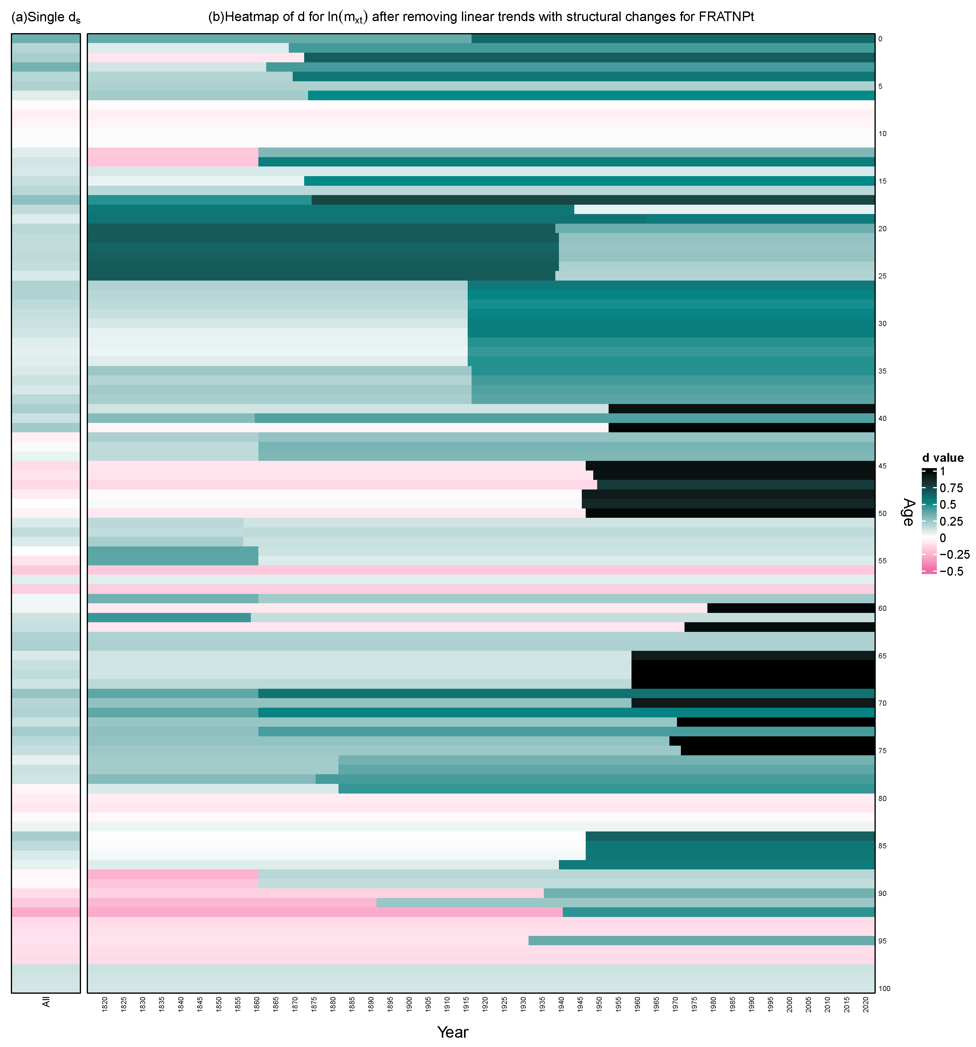
Figure 1. For French total population mortality data during 1816–2022 for ages 0–100, after adequately detrending l n ( m x t ) , t [ 1816 , 2022 ] for each age x by removing the linear trends with structural changes, we applied MR test considering structural change in persistence on the detrended time series and displayed the results in (b) as the heatmap of estimated d for each specific year and age. We also applied the Gaussian Semiparametric local Whittle estimator to estimate d s for the whole period without considering the structural change in persistence, and displayed it in (a) as a comparison to (b).
Risks 13 00225 g001
Figure 2. For Sweden total population mortality data during 1751–2022 for ages 0–100, after adequately detrending l n ( m x t ) , t [ 1751 , 2022 ] for each age x by removing the linear trends with structural changes, we applied MR test considering structural change in persistence on the detrended time series and displayed the results in (b) as the heatmap of estimated d for each specific year and age. We also applied the Gaussian Semiparametric local Whittle estimator to estimate d s for the whole period without considering the structural change in persistence, and displayed it in (a) as a comparison to (b).
Risks 13 00225 g002
Figure 3. Zoom-in heatmap of d for age-12 in Figure 1b.
Risks 13 00225 g003
Figure 4. For Sweden total population and France total population mortality data, compare the estimated d 1 , d 2 and d s for the adequately detrended l n ( m x t ) for each age x after removing linear trend with structural changes. (a) France total population during 1816–2022 for ages 0–100, (b) Sweden total population during 1751–2022 for ages 0–100).
Risks 13 00225 g004
Figure 5. For Sweden total population and France total population mortality data, plots of the estimated persistence break timepoint for each age with an observed structural change in persistence in the adequately detrended l n ( m x t ) after removing linear trend with structural changes. (a) France total population during 1816–2022 for ages 0–100, (b) Sweden total population during 1751–2022 for ages 0–100.
Risks 13 00225 g005
Figure 6. The heatmap of d clustered on ages, for French total population mortality data during 1816–2022 for ages 0–100, where d is estimated by MR test on the adequately detrended l n ( m x t ) .
Risks 13 00225 g006
Figure 7. The heatmap of d clustered on ages, for Sweden total population mortality data during 1751–2022 for ages 0–100, where d is estimated by MR test on the adequately detrended l n ( m x t ) .
Risks 13 00225 g007
Figure 8. Age clusters resulting from clustering into three clusters by the structural changes in persistence (denoted as “by SC in d”) or by the structural changes in linear trend (denoted as “by SC in LT”), for both France total population and Sweden total population. The three different colors red, yellow and blue present the three clusters. For each of the column 2, 3, 5, 6, the ages with the same color are in the same cluster.
Risks 13 00225 g008
Figure 9. The heatmap of removed linear trend with structural changes for French total population mortality data l n ( m x t ) .
Risks 13 00225 g009
Figure 10. The heatmap of d for France total population mortality data during 1816–2022 for ages 0–100; d is estimated by the MR test on the detrended l n ( m x t ) by removing simple linear trend.
Risks 13 00225 g010
Figure 11. The heatmap of d for Sweden total population mortality data during 1751–2022 for ages 0–100; d is estimated by MR test on the detrended l n ( m x t ) by removing simple linear trend.
Risks 13 00225 g011
Table 1. Compare the results of M, M1, M2 applied to the simulated data. Column 1 and 2 are the results for all the simulated time series which are assumed to have a change in persistence; column 3 and 4 are the results for all the simulated time series with the assumption of no change in persistence.
Change in d AssumedNo Change in d Assumed
%(dSC)67.19%%(dSC)33.40%
m ( d 1 ^ ) d 1 −0.0436 m ( d 1 ^ ) d s −0.1609
m ( d 2 ^ ) d 2 −0.1670 m ( d 2 ^ ) d s −0.0826
m ( d s ^ . M 1 ) d 1 −0.1153 m ( d s ^ . M 1 ) d s −0.3263
m ( d s ^ . M 1 ) d 2 −0.4569
m ( d s ^ . M 2 ) d 1 0.7052 m ( d s ^ . M 2 ) d s 0.5649
m ( d s ^ . M 2 ) d 2 0.3635
Disclaimer/Publisher’s Note: The statements, opinions and data contained in all publications are solely those of the individual author(s) and contributor(s) and not of MDPI and/or the editor(s). MDPI and/or the editor(s) disclaim responsibility for any injury to people or property resulting from any ideas, methods, instructions or products referred to in the content.