Article

Effects of Traditional Reinsurance on Demographic Risk Under the Solvency II Framework

Department of Mathematics for Economic, Financial and Actuarial Sciences, Università Cattolica del Sacro Cuore, Largo Gemelli 1, 20123 Milan, Italy
*
Author to whom correspondence should be addressed.
Risks 2025, 13(10), 203; https://doi.org/10.3390/risks13100203
Submission received: 18 July 2025 / Revised: 23 September 2025 / Accepted: 11 October 2025 / Published: 14 October 2025

Abstract

This paper investigates the role of proportional reinsurance as a practical and flexible tool for managing demographic risk in life insurance, with a focus on its impact on both the Solvency Capital Requirement (SCR) and expected profitability. While much of the existing literature focuses on mortality modeling or longevity-linked reinsurance instruments, this paper proposes a novel framework for analyzing traditional proportional reinsurance structures within the Solvency II market-consistent valuation environment. The framework integrates proportional reinsurance into the valuation of liabilities and the calculation of Solvency Capital Requirement, beginning with an outline of cash flow structures and their valuation under Solvency II principles. A key contribution is the introduction and decomposition of the net of reinsurance Claims Development Result (CDR), which allows us to assess the dual impact of reinsurance on risk mitigation and profit transfer. Through numerical analysis, we show how proportional reinsurance can effectively reduce capital requirements while quantifying the trade-off in expected profit transferred to the reinsurance company, with insights into how different reinsurance treaties affect capital efficiency and profitability.

1. Introduction

The Solvency II Directive (see European Parliament and Council 2014, 2009), implemented in 2016, has fundamentally reshaped the European insurance regulatory framework. Among its many innovations, Pillar I introduced the market-consistent actuarial valuation of assets and liabilities, as well as risk-based rather than factor-based capital requirements. With respect to valuation, assets and liabilities must be assessed at their current exit value, i.e., the price at which they could be transferred in an arm’s length transaction between willing parties. Non-hedgeable liabilities, such as insurers’ technical provisions, must be calculated as the sum of the Best Estimate and the Risk Margin. The former corresponds to the discounted expected value of future cash flows under the relevant risk-free curve, while the latter reflects the compensation a third party would demand in order to assume the insurer’s obligations.
Concerning the capital requirement demographic risk, especially mortality and longevity risk, plays a central role in the valuation of traditional life insurance liabilities. Although the Solvency II framework provides solid bases for measuring such risks, there remains a growing need to develop practical tools not only for quantifying these risks, but also for mitigating them in a way that aligns with solvency capital requirements.
The valuation of life insurance policies with linked benefits, whose return is tied to a financial variable (such as stocks, indices, or investment funds), has been extensively studied in the literature. Within a traditional deterministic framework, the problem is rather straightforward: the value coincides with the present value of future cash flows (see Brennan and Schwartz 1976, 1979). In addition, a variety of principles for pricing such hybrid products have been proposed (see Bacinello 2001; Barigou et al. 2019; Barigou and Delong 2022; Møller 1998, 2002). More recently, Deelstra et al. (2020) have introduced a novel decomposition method that clearly distinguishes between risks that can be hedged in financial markets, risks that can be diversified through pooling, and a residual component that must be assessed in line with solvency guidelines. As for the computation of the Solvency Capital Requirement (SCR) for demographic risk, several approaches have been put forward to move beyond the traditional factor-based methodology and towards a genuinely risk-based framework. The authors in (Savelli and Clemente 2013) develop a cohort-based approach consistent with local Generally Accepted Accounting Principles, while (Wüthrich et al. 2010) implement a market-consistent actuarial valuation for capital requirement purposes. This issue is further investigated in (Clemente et al. 2022) and (Clemente et al. 2024a), which concentrate exclusively on the idiosyncratic component of demographic risk, and in (Clemente et al. 2024b), where a model specifically designed for equity-linked policies is proposed.
Although the quantification of risk is crucial for insurance companies, its mitigation is equally important. In this regard, the present work considers reinsurance for a homogeneous portfolio of policyholders holding life insurance contracts, and formally analyzes, from a mathematical standpoint, the effects of reinsurance (see Albrecher et al. 2017; Besson et al. 2009; Chi et al. 2017). Recent contributions include (Yang and Zhou 2023), who develop a surrogate simulation approach based on thin-plate regression splines to efficiently approximate the SCR under stochastic mortality, and (Meyricke and Sherris 2014), who evaluate indemnity-based longevity swaps as a reinsurance solution under Solvency II. These studies highlight how recent research has increasingly focused on specialized modeling techniques for mortality- or longevity-linked reinsurance instruments.
This paper contributes to the existing literature by introducing a novel, flexible, and analytically grounded framework for evaluating proportional reinsurance as a strategic tool for managing demographic risk in traditional life insurance portfolios. While recent studies have explored stochastic modeling of mortality risk or specific longevity-linked reinsurance instruments, the use of standard proportional reinsurance treaties, such as quota-share and surplus, as a means to balance profitability and capital efficiency under Solvency II has received comparatively less attention in the literature. This gap in the literature is addressed by our approach, which provides new insights into the effectiveness of proportional reinsurance within the Solvency II framework.
The key contribution of this work lies in the development of a model that integrates proportional reinsurance into the valuation of liabilities and the calculation of solvency capital requirements. By building on the concept of the Claims Development Result (CDR), we establish a link between profitability and solvency over a one-year time horizon. Secondly, we perform a sensitivity analysis to assess the impact of different reinsurance treaties on both the demographic component of the Solvency Capital Requirement (SCR) and the expected profitability of the insurer. Finally, we analyze how alternative pricing methodologies and portfolio characteristics, such as the heterogeneity of insured sums, influence the relative effectiveness of reinsurance structures. This allows for a comparison of quota-share and surplus treaties under varying market and risk conditions, and provides guidance on identifying the optimal reinsurance strategy.
Methodologically, our approach is grounded in actuarial modeling principles and builds on the concept of the valuation portfolio, allowing us to model cash flows on a cohort basis while maintaining compliance with market-consistent valuation guidelines. The model is designed to be highly adaptable and applicable to a wide range of traditional life insurance contracts. Numerical examples are provided to illustrate the practical implications of the proposed framework across different reinsurance scenarios and portfolio configurations. In doing so, this work contributes to both the academic literature and the practical field of insurance risk management by offering a comprehensive toolkit for the strategic use of reinsurance under Solvency II. The proposed methodology helps insurers identify optimal reinsurance structures that align with both regulatory constraints and business objectives, ultimately supporting more informed and capital-efficient decision-making.
The use of reinsurance by an insurance undertaking entails exposure to counterparty default risk. In this regard (see Art. 105 of European Parliament and Council (2009) and Arts. 189 et seq. of European Parliament and Council (2014)), the Standard Formula prescribes the calculation of the SCR for counterparty default risk as a function of the Loss Given Default (LGD) and the Probability of Default (PD). The former depends on the recoverables (understood as the Best Estimate of amounts recoverable from the reinsurance arrangement) and on the risk-mitigating effect on underwriting risk of the reinsurance arrangement. The PD, on the other hand, depends on the credit assessment of the reinsurer. Since this work does not focus on the calculation of the SCR for counterparty default risk, we only specify that the overall SCR of the insurance undertaking will include both the SCR for demographic risk and the SCR for counterparty default risk, with the latter being readily computable using the quantities introduced in the paper, primarily the Best Estimate of the liabilities ceded to the reinsurer.
From a numerical perspective, the analysis reveals how the interaction between reinsurance structures and portfolio characteristics can substantially affect both capital requirements and profitability. In particular, the study shows that the degree of heterogeneity in the insured sums plays a pivotal role, as it directly impacts the diversification of demographic risk and, consequently, the effectiveness of different reinsurance arrangements. The results also underscore the sensitivity of outcomes to the adopted reinsurer pricing principles, highlighting non-trivial trade-offs between capital relief and profitability that become especially relevant when reinsurance is priced under volatility-based rules. These insights provide a richer understanding of how reinsurance design and pricing interact, offering practical implications for insurers operating within a Solvency II framework.
The remainder of the paper is structured as follows: Section 1 introduces the modeling assumptions. Section 3 describes the cash flow structure and the cohort-based approach. Section 4 details the valuation of Best Estimate liabilities. Section 5 incorporates the reinsurance mechanism into the CDR formulation. Section 6 elaborates on the reinsurance structures and pricing methodologies. Section 7 presents numerical analyses, and Section 8 concludes with final remarks. Mathematical details and proofs are provided in the Appendices Appendix AAppendix C.

2. Preliminaries

We define the probability space Ω , F , P , where Ω is the sample space, P is the probability measure, and F t denotes the σ -algebra representing the accumulation of information over time.
A filtration F : = F t t = 0 , , n is defined as a non-decreasing sequence of σ -algebras on ( Ω , F , P ) such that:
, Ω = F 0 F 1 F n F .
We then refer to Ω , F , P , F as the filtered probability space. We now define two subfiltrations, T : = T t t = 0 , , n and G : = G t t = 0 , , n , each of which is a subset of the filtration F and represents a smaller collection of information. These two subfiltrations are related to insurance technical events and financial events, respectively.
We assume that, at each time t, F t is generated by both T t and G t , that is T t , G t F t , and that T t and G t are independent with respect to the probability measure P .
We denote the F -adapted vector of cash flows as X = ( X 0 , X 1 , , X n ) ,1 where each component X t is measurable with respect to the σ -field F t for t = 0 , 1 , , n .
Consider two vectors of random variables, X and Y , both of dimension n × 1 . We assume the following conditions:
E t = 0 n X t 2 < ,
E t = 0 n X t · Y t < .
Assumption 1 
(Valuation functional and deflator). We assume the existence of a valuation functional Q such that the mapping X Q t ( X ) assigns a monetary value Q t ( X ) R to every vector of cash flows X . This value can be interpreted as the price or worth of X at time t.
Taking advantage of the Riesz-Fréchet representation theorem, for every Q there exists a unique random vector φ ( P , F ) such that the inner product with this vector yields the same value as Q t X ( t ) . This is expressed as:
Q t X ( t ) = 1 φ t · E t s = t n φ s · X s .
The notation X ( t ) 2 is used to denote a generic vector X ( t ) : = X τ τ = t , , n .
In this setting, φ represents the F -adapted vector of state-price deflators. We remark that the vector is normalized such that φ 0 = 1 , providing a baseline for discounting future cash flows, and each of its components is strictly positive and square-integrable. Moreover, the vector φ is a ( P , F ) -martingale, and in the case of a complete market, it is unique. As a result of these properties, each deflator allows the assignment of a market-consistent value to each cash flow X h , with h 0 , , n . Consequently, it is possible to represent the technical provision R t ( h ) at time t, where t 0 , , h , for outstanding cash flows as:
R t ( h ) = Q t X ( h ) = 1 φ t · E t s = h n φ s · X s .
We clarify that by the term technical provision, we are referring only to one of its components, specifically the one related to the Best Estimate. In other words, the additional term required by Solvency II regulation, related to the Risk Margin (see European Parliament and Council 2009), is excluded from our analysis. This choice is motivated by the fact that our focus is on describing the demographic risk only. The definition of the Risk Margin, according to the Cost of Capital approach proposed by the regulation, involves considering additional sources of risk, such as operational, default, and other life underwriting risks. Therefore, to achieve our goal, the Risk Margin must be excluded from the valuation. Furthermore, we recall that, to avoid computational burden, the regulation (see European Parliament and Council 2014) requires the exclusion of the Risk Margin from the computation of the SCR, which is the primary focus of this article.
Exploiting the concept of the independent split of filtrations defined above, the state-price deflator can be expressed as:
φ t = φ t T · φ t G .
The distinction between the two factors will be revisited later, as it allows for the separate treatment of the technical and financial aspects.

3. The General Framework

We develop a model based on a traditional term insurance policy, issued at time t = 0 and maturing at time t = n , characterized by constant annual premiums. At the inception date, we consider a cohort of l 0 policyholders, all with the same entry age x, each having an initial sum insured c k , 0 , where k = 1 , , l 0 .
Definition 1 
(Cohort). We define a cohort as a group of policyholders who share the same characteristics relevant to our analysis, such as the same entry age x, the same contract type, the same premium payment method, etc., except for the amount of the sum insured, which may vary across policyholders.
This choice allows us to analyze the risk by focusing on the main factors that drive the variability in the risk profile within a given population of policyholders, such as the Sum-at-Risk and the variability of the sums insured.
Each contract guarantees the beneficiary a predefined amount if the insured, aged x, dies before reaching the age x + n . Assuming that each policyholder has a deterministic sum insured, for a general traditional term insurance policy, the stochastic nature of the benefit arises from the randomness of the policyholder’s survival, making the future payout uncertain. Although the main formulas have been presented for a term insurance contract, the same approach also applies to other types of traditional life insurance contracts.
We assume that the survival status of each policyholder at each time step τ is modeled using a Bernoulli random variable (r.v.) I k , τ L ,3 which takes the value 1 if the policyholder survives the period τ , τ + 1 , indicating that the contract remains in force, and 0 if the policyholder dies within the year. At any given time t 0 , , n , the random sum insured C k , t is defined as follows:
C k , t : = c k , 0 · τ = 0 t 1 I k , τ L .
Given that policyholders within the same cohort share identical characteristics, particularly their age at the inception of the contract, we can assume that their survival indicators are identically distributed Bernoulli random variables. We also assume that, even knowing the actual probability of death for each individual policyholder, their deaths are (conditionally) independent (see Hanbali et al. 2019; Milevsky et al. 2006). Therefore, we refer to these random variables as conditionally independent and identically distributed. The stochastic sum insured at the cohort level, i.e., considering l 0 policyholders, at time t can be calculated as:
C t = k = 1 l 0 C k , t .
In addition to the cash flows related to benefit payments, we extend our analysis to include acquisition expenses, which are associated with the compensation of the distribution channel, and management expenses, which cover the ongoing costs of administering and servicing insurance policies. These expenses are defined as constant percentages, γ A and γ M , applied to the sums insured.4 The cost of these expenses is typically passed on to the policyholder by incorporating additional loadings in the premium definition,5 which account for acquisition expenses, γ { A } , and management expenses, γ { M } .
Assumption A2 
(Cash flows timing). In modeling the cash flows for the cohort of policyholders, we establish a framework based on the following assumptions:
1. 
Gross premiums are collected at the beginning of each year, at time t + , for every policyholder who is still alive.
2. 
Acquisition expenses are fully paid at the inception of the contract (i.e., t = 0 ), while management expenses are paid at the beginning of each period, at time t + , provided the policyholder is still alive.
3. 
Death benefits due to beneficiaries for claims occurring within the period ( t , t + 1 ] are paid at the end of the time interval, i.e., at time t + 1 .
Considering a generic time t { 0 , , n 1 } , the vector of cash flows X ( t ) : = X τ τ = t , , n is decomposed into income X τ in and outflow X τ out components, in accordance with the timing assumptions mentioned earlier and the market-consistent valuation principles of Solvency II:
X τ = X t out : A + X t out : M X t in : pure + X t in : A + X t in : M if τ = t , X τ out : pure + X τ out : M X τ in : pure + X τ in : A + X τ in : M if t < τ < n , X n out : pure if τ = n .
In Formula (9), each cash outflow is split into its pure component, denoted X τ out : pure , which represents the benefits the insurance company must pay to beneficiaries for claims occurring within the one-year period. The outflows also include two expense components: X τ out : M , for management expenses and X τ out : A , for acquisition expenses.
Regarding the cash inflows, there is no need to differentiate between the different components as the full premium is paid at once. However, we introduce the notations X τ in : pure , X τ in : A and X τ in : M which will be employed in subsequent sections to represent the inflows corresponding to pure premiums, acquisition expense loadings, and management expense loadings.
We split the generic cash flow into a hedgeable G τ -measurable part and an unhedgeable T τ -measurable part:6
X τ out = k = 1 l 0 c k , 0 · γ A · 1 t = 0 · B 0 out , 0 + k = 1 l 0 C k , t · γ M · B t out , t if τ = t , k = 1 l 0 C k , τ 1 · I k , τ 1 B · B τ out , τ + k = 1 l 0 C k , τ · γ M · B τ out , τ if t < τ < n , k = 1 l 0 C k , n 1 · I k , n 1 B · B n out , n if τ = n ,
and
X τ i n = k = 1 l 0 C k , τ · p + γ A + γ M · B τ in , τ if t τ < n , 0 if τ = n ,
where p is the pure premium rate.
Regarding the pure component, the benefit for a generic policyholder depends on the value of the sum insured at the beginning of the one-year period and a Bernoulli random variable I k , τ 1 B . The parameter of I k , τ 1 B depends on the type of insurance contract. Here, as we consider a cohort of term insurance policies,7 we have I k , τ 1 B = I k , τ 1 D = 1 I k , τ 1 L , meaning it takes the value 1 if the policyholder dies within the year τ 1 , τ , and 0 otherwise.8
We assume that within the cohort the insurance technical variables I k , τ 1 B are conditionally i.i.d. Bernoulli random variables described by a T τ -measurable stochastic parameter Q x + τ 1 with expected value equal to E P Q x + τ 1 = q x + τ 1 . The r.v. Q x + τ 1 depends exclusively on the time instant and not on individual policyholder, hence for each τ 1 , , n , the joint death probability of two generic policyholders h , k 1 , , l 0 , with h k , can be represented as follows:
P I h , τ 1 D = 1 , I k , τ 1 D = 1 | Q x + τ 1 = P I h , τ 1 D = 1 | Q x + τ 1 · P I k , τ 1 D = 1 | Q x + τ 1 = q x + τ 1 2 .
We aim to build a model framework coherent with the market-consistent valuation prescribed by Solvency II, hence q x + τ 1 is defined as the realistic probability of death (second-order9 mortality probability) for a policyholder aged x at inception.10 Given a generic τ 0 , , n , we assume that B τ out , t t = 0 , , n is a G -adapted stochastic process representing the price of a Zero Coupon Bond (ZCB) B τ out maturing at time τ , used to replicate a unitary outflow. We clarify that the superscript t denotes that it is the price of B τ out at time t.
Formula (11) describes the cash inflows generated by the collection of constant annual premiums paid by each k-th policyholder who is alive at time τ . As for the outflows, we define the G -adapted stochastic processes B τ in , t t = 0 , , n representing the price process of the Zero Coupon Bond B τ in with maturity τ used to replicate a unitary inflows.
A compact representation of all cash flows, introduced in Formulas (9)–(11), is shown in Table 1. To distinguish between portfolio-level and individual-level values, we introduce the notations X k , τ out : pure , which denote the benefit-related cash outflow attributable to the k-th policyholder. Similarly, the inflows X k , τ in : pure , X k , τ in : A , and X k , τ in : M correspond to the amounts paid by the same policyholder for pure premiums, acquisition expenses, and management expenses, respectively.
More generally, X k , τ can be regarded as the cash flow for each component (whether inflow or outflow) associated with the k-th policyholder.

4. The Cohort Valuation Portfolio

Consider a Valuation Portfolio (VaPo, see Wüthrich et al. 2010) as a portfolio of financial instruments designed to replicate a specific series of future cash flows. In this section, we outline the steps to construct and define the value of a VaPo in a way that ensures consistency with the cohort approach.
  • Step 1 Choice of financial instruments.
    According to Formula (9), the distinct timing of cash flows necessitates separate consideration of inflows and outflows at time t. Each can be replicated using respective portfolios of financial instruments. We consider a cohort of term insurance policies with constant capital and fixed annual premiums. At each time t, the inflows and outflows are replicated using ZCBs, denoted as B t in and B t out .
  • Step 2 Determination of the number of portfolio shares to replicate cash flows.
    Once the financial instruments are selected, we determine the quantity of each required to replicate the future cash flows X ( t ) :
    X ( t ) V a P o t X ( t ) = = k = 1 l 0 s = 0 n t 1 C k , t · E t P h = 0 s 1 I k , t + h L · I k , t + s B · B t + s + 1 out + E t P h = 0 s 1 I k , t + h L · γ M · B t + s out + k = 1 l 0 c k , 0 · γ A · 1 t = 0 · B 0 out k = 1 l 0 s = 0 n t 1 C k , t · E t P h = 0 s 1 I k , t + h L · p + γ A + γ M · B t + s in .
  • Step 3 The accounting principle used to value financial instruments.
    Each financial instrument is valued according to the selected accounting principle. In this paper, we adopt a fair value approach under the Solvency II framework, meaning that each instrument is valued at its current market price. We denote this accounting principle by E t , with t { 0 , , n } , and define the accounting value of the cash flows as:
    X ( t ) E t V a P o t X ( t ) = = k = 1 l 0 s = 0 n t 1 C k , t · E t P h = 0 s 1 I k , t + h L · I k , t + s B · E t B t + s + 1 out + E t P h = 0 s 1 I k , t + h L · γ M · E t B t + s out + k = 1 l 0 c k , 0 · γ A · 1 t = 0 · E 0 B 0 out k = 1 l 0 s = 0 n t 1 C k , t · E t P h = 0 s 1 I k , t + h L · p + γ A + γ M · E t B t + s in .
    Introducing the prices of the financial instruments, we have:
    X ( t ) E t V a P o t X ( t ) = Q t X ( t ) = = k = 1 l 0 s = 0 n t 1 C k , t · E t P h = 0 s 1 I k , t + h L · I k , t + s B · B t + s + 1 out , t + E t P h = 0 s 1 I k , t + h L · γ M · B t + s out , t + k = 1 l 0 c k , 0 · γ A · 1 t = 0 · B 0 out , 0 k = 1 l 0 s = 0 n t 1 C k , t · E t P h = 0 s 1 I k , t + h L · p + γ A + γ M · B t + s in , t .
We propose a definition of the cohort Best Estimate liabilities that is consistent with both the market-consistent valuation framework of Solvency II (see European Parliament and Council 2009) and the features of the contract under consideration: R t : = Q t X ( t ) .
Definition 2 
(Premium calculus and cohort VaPo protected). By replacing insurance technical risks with their conditional expectations at time t = 0 , and assuming that financial instruments are valued at market prices, we define the market value of the VaPo protected as follows:
E 0 V a P o 0 prot X ( 0 ) out : pure X ( 0 ) in : pure = = k = 1 l 0 s = 0 n 1 c k , 0 · E 0 P h = 0 s 1 φ ˜ h + 1 T · I k , h L · I k , s B · E 0 B s + 1 out k = 1 l 0 s = 0 n 1 c k , 0 · E 0 P h = 0 s 1 φ ˜ h + 1 T · I k , h L · p · E 0 B s in .
Hence, the annual pure premium rate p can be determined by solving the equation:
E 0 V a P o 0 prot X ( 0 ) out : pure X ( 0 ) in : pure = 0 .
In Formula (13), we apply the concept of a deflator11 to transition from the real-world probability measure to a first-order measure, thereby incorporating a more prudent, risk-averse valuation perspective. It is important to note that this work focuses exclusively on demographic risk, explicitly excluding financial risks. As a result, we consider only the technical deflator, with the implicit assumption that φ ˜ G = 1 since financial cash flows are already discounted throughout the accounting principle.12
To derive the gross premium, we add loadings for contract-related expenses to the pure premium. Assuming deterministic expenses represented by constant coefficients γ A and γ M , applied to the sum insured, we define the loading coefficients for acquisition and management expenses, denoted by γ { A } and γ { M } , based on the equivalence principle (Olivieri and Pitacco 2015), under second-order (i.e., non-prudent) assumptions:13
E 0 P s = 0 n 1 C k , s · γ A · B s in , 0 = k = 1 l 0 c k , 0 · γ A · B 0 out , 0 , γ M = γ M .
Neglecting the risk associated with revisions to second-order expenses assumptions, we define the Best Estimate liabilities for expenses at time t, denoted by R t E ,14 as the provision required to cover any mismatch between expenses payments, X ( t ) out : A + X ( t ) out : M , and the corresponding expense loadings, X ( t ) in : A + X ( t ) in : M . The cost of managing contracts for surviving policyholders is fully hedged by the corresponding management expense loadings, resulting in no timing mismatch. In contrast, acquisition expenses are incurred at inception, while the related loadings are collected over the lifetime of the contract through premium payments. Accordingly, R t E is given by:
R t E : = E t V a P o t X ( t ) out : A X ( t ) in : A .
For each t > 0 , R t E represents the current market value of a valuation portfolio that replicates the negative difference between the expected present value of future acquisition expenses, which is zero, and the expected present value of the corresponding loadings. The latter can be interpreted as a credit the company holds against its policyholders.
For each t 0 , , n 1 , we define the total Best Estimate15 R t as the market value of a VaPo designed to replicate the difference between the expected present value of future cash outflows and the expected present value of future cash inflows. A compact formulation is presented here, while the full expression is provided in Formula (A1), Appendix A.
R t = E t V a P o t X ( t ) out X ( t ) in .
During the premium payment period, and until all the loadings for acquisition expenses have been collected, the total reserve is lower than the pure reserve. This difference is attributable to the expenses reserve R t E , which is particularly significant in the early years of the contract.

5. Demographic Risk and Solvency

As mentioned earlier, Solvency II introduced a risk-based framework to ensure adequate policyholder protection across the European insurance market. The regulation requires the SCR to be calibrated to account for all quantifiable risks faced by insurance and reinsurance undertakings (see Article 101 European Parliament and Council 2009).
Our analysis focuses on the capital requirement for demographic risk. Within the life underwriting risk module, we specifically address the mortality and longevity sub-modules. These risks are defined as the potential loss or adverse change in the value of insurance liabilities resulting from changes in mortality rates. An increase in mortality rates (or a decrease in the case of longevity risk) leads to an increase in the value of insurance liabilities.

5.1. The Model Framework

Let us consider a generic time interval ( t , t + 1 ] . At the beginning of the year t, the insurance company calculates the Best Estimate liabilities, R t , using the most up-to-date information,16 so we consider the total Best Estimate. At the beginning of the year t, the reserve is increased by deterministic premiums, X t in , paid by policyholders who are still alive, while the management costs, X t out : M , are deducted for active contracts. Additionally, in the special case of t = 0 , the entire amount of acquisition expenses related to the contracts is deducted from the total resources available.
Let V t + 1 denote the market value at the end of the year ( t , t + 1 ] , of the total amount available in t, given by R t + X t in : pure + X t in : A X t out : A . Thus, V t + 1 represents the valuation portfolio V a P o t X t , purchased at time t at its market price R t , increased by the inflows collected and reduced by the outflows paid at time t, and revalued at time t + 1 . We define it as follows:
V t + 1 : = E t + 1 V a P o t X ( t ) out : pure X ( t + 1 ) in : pure X ( t + 1 ) in : A .
A compact formulation is presented here, while the full expression is provided in Formula (A2), Appendix A.
At time t + 1 , V t + 1 must cover the cost of claims and the updated total Best Estimate reserve, R t + 1 , which reflects the latest demographic and financial information. Accordingly, we define the Claims Development Result (CDR) as follows:
C D R t + 1 : = V t + 1 X t + 1 out : pure R t + 1 .
Formula (17) reflects two sources of uncertainty: idiosyncratic risk and trend risk. Idiosyncratic risk refers to accidental mortality, i.e., the random fluctuation in the number of deaths during the year. This affects both the benefits X t + 1 out : pure and the Best Estimate R t + 1 . Trend risk arises from the volatility of technical assumptions and the possibility of revising initial estimates based on new information. It affects the Best Estimate computed at the end of the year based on the new filtration T t + 1 . Trend risk typically reflects observed changes in mortality or longevity trends.
In Formula (17), financial information is updated at time t + 1 using the filtration G t + 1 . The available resources V t + 1 are based on technical information contained in T t , whereas the new total Best Estimate reflects the updated technical information in T t + 1 .
Let us define R t + 1 * as the Best Estimate computed at time t + 1 , under the assumption that technical risk is still conditioned on the information available at time t, i.e., based on T t . Specifically, R t + 1 * represents the market value, at time t + 1 , of a valuation portfolio that replicates the difference between the expected present value of future outflows and the expected present value of future inflows, where the expectation is taken under the assumptions that the information available at time t remains valid, and no revisions to the technical assumptions occur during the period.
R t + 1 * : = E t + 1 V a P o t X ( t + 1 ) out X ( t + 1 ) in .
Accordingly, the two components of the CDR can be expressed as follows:
C D R t + 1 Idios : = V t + 1 X t + 1 out : pure R t + 1 * ,
C D R t + 1 Trend : = R t + 1 * R t + 1 .

5.2. The Idiosyncratic Risk

Starting from Formula (19), the one-year profit or loss attributable to idiosyncratic risk can be expressed in a more compact form, as shown below. The proof is provided in Appendix A:
C D R t + 1 Idios = k = 1 l 0 C k , t · E t P I k , t B I k , t B · η t + 1 ,
where η t + 1 = ( B t + 1 out , t + 1 β t + 1 ) , and β t + 1 denotes the Best Estimate rate for a generic policyholder, calculated at time t + 1 , under the assumption that the technical parameters estimated at time t remain unchanged. The quantity β t + 1 is given by:
β t + 1 = s = 0 n t 2 E t P h = 0 s 1 I k , t + h + 1 L · I k , t + s + 1 B · B t + s + 2 out , t + 1 s = 0 n t 2 E t P h = 0 s 1 I k , t + h + 1 L · p + γ A · B t + s + 1 in , t + 1 .
Since policyholder deaths within the cohort are conditionally independent and identically distributed, β t + 1 is identical for all policyholders.
Formula (21) shows that the one-year profit or loss from idiosyncratic risk is driven by the volatility around the estimated demographic assumption. More precisely, it captures the difference between the expected value of benefits at time t and the actual benefits observed at time t + 1 . The first factor, k = 1 l 0 C k , t , is T t - measurable and acts as a scaling factor. The third term, η t + 1 , represents the Sum-at-Risk rate at time t + 1 for a generic policyholder, conditional on the filtration T t . For traditional term insurance policies, this rate is always positive.
The value of C D R t + 1 Idios may be either positive or negative, depending on whether the observed mortality is lower or higher than expected. An increase in accidental mortality during the year leads to higher benefit payments at time t + 1 and to a reduction in future premium income. In practice, the risk of unexpected benefit payments due to uncertainty in demographic assumptions is addressed during pricing, typically through a safety loading applied to the pure premium. Furthermore, insurers must account for the effect of mortality deviations on future acquisition expense loadings, as these can influence the recovery of initial acquisition costs.

5.3. Characteristics of Demographic-Idiosyncratic Risk

We now examine the main characteristics of the C D R t + 1 Idios . Given the technical and financial information available at time t, represented by the filtration F t , the idiosyncratic component of the CDR has zero expectation:  
E t P C D R t + 1 Idios = 0 .
This follows directly from the Tower Property (law of iterated expectations). From an actuarial perspective, it implies that if the demographic assumptions are fixed at time t, then, on average, the initial amount available at the beginning of the year, valued at t + 1 , will cover the expected benefit payments for ( t , t + 1 ] , update the Best Estimate at time t + 1 , and partially recover acquisition costs. Consequently, no profit or loss arises, on average, from annual idiosyncratic risk.
For the volatility, we obtain the following expression, with the proof provided in Appendix B:
V a r P C D R t + 1 Idios | F t = l t · q x + t · 1 q x + t · C ¯ t 2 + l t 2 · C ¯ t 1 2 · σ Q x + t 2 · E P η t + 1 2 | G t ,
where C ¯ t j denotes the j-th raw moment of the distribution of the sums insured for policies still in force at time t.
The variance of the idiosyncratic risk can be decomposed into two components. The first term, l t · q x + t · ( 1 q x + t ) · C ¯ t 2 , is diversifiable by increasing portfolio size. The second term, l t 2 · ( C ¯ t 1 ) 2 · σ Q x + t 2 , arises from the stochastic nature of the Bernoulli parameter and represents a non-diversifiable systematic risk.
Volatility increases with both cohort size and death probability, although for extreme ages (when q k , t 0.5 ), this relation reverses. The coefficient of variation of the sums insured plays a key role in demographic risk volatility and in determining the capital requirement, especially for high-value policies. Such policies may create concentration risk, where large individual claims disproportionately affect the portfolio. Reinsurance is commonly used to mitigate this exposure, as discussed in Section 6. Finally, total volatility also depends on the magnitude of the Sum-at-Risk rate, which in turn is determined by the type of contracts within the cohort.
Our aim is to exploit the properties of the previously defined CDR to explicitly quantify the SCR and to propose an alternative methodology compared to the Solvency II standard formula. Specifically, the idiosyncratic component of the SCR, denoted S C R Idios , is calculated as the negative 0.5% quantile of the distribution of C D R t + 1 Idios .

6. Managing Demographic Risk and Reinsurance Strategy

We define a reinsurance treaty as a contractual agreement in which the ceding company, or primary insurer, pays a reinsurance premium in exchange for transferring a portion of the risks it has underwritten. In the context of traditional life insurance, where the benefits payable upon the occurrence of an insured event are typically predefined,17 the most common arrangements are proportional reinsurance contracts, which generally apply to the entire portfolio.
Under a proportional reinsurance treaty, the premium paid to the reinsurer is usually expressed as a fixed percentage of the whole premium collected by the primary insurer. Although the primary insurer bears all expenses, a corresponding share of the expense loadings it receives is transferred to the reinsurer. This structure aligns the reinsurer’s revenue with the insurer’s pricing assumptions, both in terms of risk assessment and expected profitability.
Proportional treaties often include a commission paid by the reinsurer to the primary insurer. This commission serves two purposes: to compensate the insurer for the excess premium ceded and to acknowledge the reinsurer’s contractual position.
In our analysis, the commission is modeled as a fixed percentage, denoted as c R E , of the ceded expense loadings, but it can readily be adapted to a sliding-scale commission structure based on the quality of the portfolio covered by the treaty. If the reinsurer fully accepts the risk price, the entire “undue” amount is returned to the primary insurer (i.e., c R E = 1 ); otherwise, a lower proportion applies.
Assumption 3 
(Net Reinsurance cash flows). In modeling the cash flows for the cohort of policyholders when a proportional reinsurance treaty is in force and in addition to the assumptions stated in (A2), we make the following assumptions:
1. 
The primary insurer bears the full cost of acquisition and management expenses.
2. 
The price of the reinsurance contract is implicitly determined by the reinsurer, with the commission percentage c R E determining the reinsurance fee.
3. 
The commission is paid by the reinsurer to the primary insurer at the beginning of each year.
In the remainder of this section, we consider two types of proportional reinsurance agreements.

6.1. Surplus Reinsurance

Surplus reinsurance is a form of proportional reinsurance in which the primary insurer establishes a retention limit, denoted d, for each contract in order to cap its exposure. For a given policy k, the proportion of risk ceded to the reinsurer is 1 α k , while the proportion retained is α k . Since the contracts within the cohort are homogeneous except for the sum insured, the ceded share varies across contracts and is given by:
α k = min d c k , 0 ; 1 .
Under this arrangement, claims with an insured sum below d are fully retained by the insurer, whereas claims exceeding d are partially ceded to the reinsurer. This structure effectively homogenizes the portfolio, as d becomes the maximum retained sum for all contracts in force.
The generic net out and in cash flows for the primary insurer under a Surplus reinsurance, denoted by X τ out , SU and X τ in , SU , are defined as follows:
X τ out , SU = k = 1 l 0 c k , 0 · γ A · 1 t = 0 · B 0 out , 0 + k = 1 l 0 C k , t · γ M · B t out , t if τ = t , k = 1 l 0 C k , τ 1 · α k · I k , τ 1 B · B τ out , τ + k = 1 l 0 C k , τ · γ M · B τ out , τ if t < τ < n , k = 1 l 0 C k , n 1 · α k · I k , n 1 B · B n out , n if τ = n ,
X τ in , SU = k = 1 l 0 C k , τ · α k · p + 1 + c R E · 1 α k α k · ( γ A + γ M ) · B τ in , τ if t τ n 1 , 0 if τ = n .
Given the cash flows, for each t 0 , , n 1 the net total reserve R t SU , accounting for Surplus reinsurance, is defined as follows:18
R t SU = E t V a P o t k = 1 l 0 α k · X k , ( t ) out : pure + X ( t ) out : M + X ( t ) out : A k = 1 l 0 α k · X k , ( t ) in : pure k = 1 l 0 α k + c R E · 1 α k · X k , ( t ) in : A + X k , ( t ) in : M .
From Formula (27), we observe that the net pure Best Estimate coincides with the pure gross reserve, with the key difference that only a portion α k of the sum insured, and the same proportion of pure premiums, is considered for each k-th policyholder. In contrast, the introduction of reinsurance impacts the structure of the expense provision compared to the gross reinsurance case. Without reinsurance, R t E is defined as the negative expected present value of future acquisition expense loadings, since annual management expenses are fully offset by the corresponding loadings collected through annual premiums. However, this perfect hedging no longer holds under proportional reinsurance. Since the commission rate is typically lower than 1, the primary insurer retains only a fraction α k + c R E · ( 1 α k ) of the expense loadings, which is insufficient to fully cover management expenses. Consequently, a reserve for management expenses arises, thereby increasing the negative reserve associated with acquisition expenses.
Following the same approach used in the case without reinsurance, we provide a definition of the CDR net of Surplus reinsurance. A detailed description of the procedure is provided in Appendix C.1.
C D R t + 1 Idios , SU = k = 1 l 0 C k , t · α k · E t P I k , t B I k , t B · η t + 1 SU ,
where η t + 1 SU = B t + 1 out , t + 1 β t + 1 SU , and β t + 1 SU is defined as follows:
β t + 1 SU = s = 0 n t 2 E t P h = 0 s 1 I k , t + h + 1 L · I k , t + s + 1 B · B t + s + 2 out , t + 1 + s = 0 n t 2 E t P h = 0 s 1 I k , t + h + 1 L · γ M α k · B t + s + 1 out , t + 1 + s = 0 n t 2 E t P h = 0 s 1 I k , t + h + 1 L · p + 1 + c R E · 1 α k α k · γ A + γ M · B t + s + 1 in , t + 1 .
It is noteworthy that Formula (28) retains the same structure as Formula (21).

6.2. Quota-Share Reinsurance

An alternative to Surplus reinsurance is the Quota-Share (QS) treaty, which is widely regarded as one of the simplest forms of reinsurance due to its fully proportional risk-sharing mechanism. Unlike Surplus reinsurance, where the retained proportion varies across policies, the QS treaty defines a fixed retention quota, denoted α , at inception; this quota applies uniformly to all contracts within the portfolio. Under this arrangement, the insurer and the reinsurer agree that, in the event of an insured loss, the reinsurer will cover a fixed proportion 1 α of the loss. Therefore, at any given time t, the total sum insured retained by the insurer is given by:
α · C t = α · k = 1 l 0 C k , t .
The reinsurance premium paid for this coverage is calculated as a proportion ( 1 α ) of the premiums collected by the primary insurer, reflecting the share of the risk ceded. Similar to Surplus reinsurance, a commission is typically negotiated to partially or fully reimburse the insurer for the ceded portion of expense loadings.
The net outflows and inflows for the primary insurer under a Quota-Share reinsurance arrangement, denoted X τ out , QS and X τ in , QS , respectively, are defined as follows:
X τ out , QS = k = 1 l 0 c k , 0 · γ A · 1 t = 0 · B 0 out , 0 + k = 1 l 0 C k , t · γ M · B t out , t if τ = t , α · k = 1 l 0 C k , τ 1 · I k , τ 1 B · B τ out , τ + k = 1 l 0 C k , τ · γ M · B τ out , τ if t < τ < n , α · k = 1 l 0 C k , n 1 · I k , n 1 B · B n out , n if τ = n ,
X τ in , QS = α · k = 1 l 0 C k , τ · p + 1 + c R E · 1 α α · ( γ A + γ M ) · B τ in , τ if t τ < n , 0 if τ = n .
The total Best Estimate net of Quota-Share reinsurance, R t QS , is defined as the sum of the gross pure reserve, scaled by the retention parameter α , and the expense reserve, which is calculated based on only a portion α + c R E · ( 1 α ) of the expenses’ loadings:19
R t QS = E t V a P o t α · X ( t ) out : pure + X ( t ) out : M + X ( t ) out : A α · X ( t ) in : pure α + c R E · 1 α · X ( t ) in : A + X ( t ) in : M .
The CDR under the Quota-Share reinsurance treaty, denoted C D R t + 1 Idios , QS ,20 represents a special case of the CDR defined for Surplus reinsurance:
C D R t + 1 Idios , QS = α · k = 1 l 0 C k , t · E t P I k , t B I k , t B · η t + 1 QS ,
where η t + 1 QS = B t + 1 out , t + 1 β t + 1 QS , and β t + 1 QS is defined as follows:
β t + 1 QS = s = 0 n t 2 E t P h = 0 s 1 I k , t + h + 1 L · I k , t + s + 1 B · B t + s + 2 out , t + 1 + s = 0 n t 2 E t P h = 0 s 1 I k , t + h + 1 L · γ M α · B t + s + 1 out , t + 1 + s = 0 n t 2 E t P h = 0 s 1 I k , t + h + 1 L · p + 1 + c R E · 1 α α · ( γ A + γ M ) · B t + s + 1 in , t + 1 .

7. Numerical Analysis

In this section, we present a numerical study to assess demographic risk in the context of a traditional term life insurance contract. We focus on the uncertainty arising from the random timing of death, which directly affects the liabilities of life insurance contracts, and analyze the distribution of outcomes induced by individual-level mortality risk.
We consider a portfolio of policies issued under fixed contractual terms with constant annual premiums and simulate the Claims Development Result (CDR) under stochastic mortality, as described in earlier sections, with a focus on assessing idiosyncratic risk. Specifically, this study aims to evaluate the effect of proportional reinsurance treaties with varying conditions on the overall risk profile of the insurance portfolio. We begin by describing the insurance product under consideration, the details of the reinsurance treaties, and the model parameters. Next, we present the results for a reference scenario, followed by a sensitivity analysis exploring the impact of different reinsurance conditions and key parameters. Additionally, we evaluate alternative traditional insurance contract structures to provide a broader analysis of the effects of risk mitigation strategies.

7.1. Simulation Parameters and Preliminary Analysis

Table 2 presents the baseline parameter values and main simulation assumptions. Our analysis focuses on a cohort consisting of 10,000 policyholders at the time of policy inception (i.e., at time 0). This cohort is selected assuming homogeneous risk within the group. We start by considering the simple case where each policyholder has an insured sum of 100,000.
At inception, all policyholders are aged 50 and the traditional term life insurance policies under consideration have a 10-year term. The valuation is conducted at time t = 5 , considering the market conditions at the end of year 2024. Consequently, at the time of valuation, the contract has a remaining duration of five years. By simulating C D R t + 1 , we assess the one-year risk over the interval between t = 5 and t + 1 = 6 . To evaluate the SCR, we then focus on the losses in the worst-case scenario at a 99.5% confidence level. The valuation time t, and thus the remaining duration of the contract, will be varied in subsequent analyses.
In the baseline scenario, the insurer considers mortality probabilities derived from the Lee-Carter model (see Brouhns et al. 2002; Lee 2000) to be realistic. However, for pricing purposes, aiming to ensure a positive expected profit, the insurer adopts a prudential demographic table based on second-order mortality rates increased by 10%.
The policy includes a technical rate of 2% used for premium computation, which implies an implicit financial guarantee. Unlike the previous analysis, this guarantee is embedded in the policy, influencing the premium structure and the overall risk profile. This addition introduces a financial component to the modeling, while maintaining a focus on the demographic risk associated with term insurance.
In this scenario, we obtain a pure premium rate p of 0.32% and a total premium rate of 0.53%. Due to the prudential assumptions used in the premium calculation, the initial Best Estimate is negative, resulting in a profit of 0.275% of the insured sum for each policyholder at inception.
In the case of reinsurance treaties, the profit depends on the premium ceded to the reinsurer and the commission paid by the reinsurer. In this scenario, since there is no variability in the insured sums, both quota-share and surplus reinsurance treaties behave in the same way (i.e., α k = α k ). Furthermore, since c R E has been set equal to 1, the profit is reduced by a factor of 1 α = 10 % , resulting in a net reinsurance profit of 0.2475% of the insured sum per each policyholder at inception (see Table 3).
The distributions of C D R Idios , gross and net of reinsurance, are obtained using the R software environment (see R Core Team 2023, version 4.5.1), based on 10 million Monte Carlo simulations. The mortality model and the bootstrap procedure are implemented with the help of the StMoMo package (Villegas et al. 2018). Due to the relatively slow execution of the bootstrap estimation, primarily caused by the computational intensity of the functions provided by StMoMo, we verified that a moderate number of bootstrap iterations is sufficient to yield stable outcomes. In particular, 1000 bootstrap simulations are adequate to achieve convergence in the distribution of Q x + t . As a result, we limit the number of iterations for the parametric bootstrap to 1000 and subsequently resample the resulting parameters 10 million times. We maintain the full set of 10 million simulations for the generation of Bernoulli random variables, the modeling of financial components, and the trend risk refitting. A large number of simulations are required to obtain accurate results, especially for the estimation of extreme quantiles. Nevertheless, we observed that the SCRs remain reasonably stable even with 1 million simulations.
Focusing on the characteristics of C D R Idios , as expected, we observe a 10% reduction in the standard deviation, while the skewness remains unaffected by reinsurance. As a result, the capital requirement is also reduced by 10%. A final observation concerns expenses: their inclusion leads to a slight increase in the total Sum-at-Risk rate, which in turn raises the capital requirement. Specifically, when considering only the pure component, the S C R I d i o s decreases from 1665.77 to 1658.63 (thousands of euros).
We also analyze the impact of using alternative risk measures and confidence levels. For instance, when the Expected Shortfall at the 99% confidence level is applied, as prescribed by the Swiss Solvency Test (see Dacorogna 2018), a slight increase in required capital is observed, which is attributable to the negative skewness of the CDR distribution. When the confidence level is maintained at 99.5% but the risk measure is changed from Value at Risk to Expected Shortfall, the increase in capital exceeds 15%, highlighting the sensitivity of the SCR to the chosen risk measure. However, in all cases, the relative capital reduction achieved through reinsurance remains constant at 10%. This is because, under the current scenario, neither treaty has an impact on the skewness of the CDR distribution.

7.2. Baseline Analysis and Sensitivities

With respect to Table 2, we now introduce the variability in sums insured, a key factor that influences both the overall variability and the SCR. Each policyholder is assigned a unique sum insured, sampled from a log-normal distribution with a mean of 100,000 and a standard deviation equal to twice the mean. The vector of individual sums insured remains fixed throughout all simulations. This distribution is highly skewed, which reflects the potential impact of high-net-worth individuals, whose deaths can lead to substantial financial losses, particularly in moderately sized cohorts. Additionally, we fix for Surplus reinsurance a retention limit d equal to 250,000 euros. This scenario will serve as the baseline for subsequent sensitivity analyses.
The main results are presented in Table 4. Notably, the heterogeneity in insured sums results in more than double the standard deviation and nearly seven times the absolute value of skewness. Consequently, there is a significant increase in the capital requirement, which is over three times higher than in the scenario where all policyholders have the same sum insured.
Additionally, the two reinsurance treaties now exhibit different effects. Specifically, the retained percentage for policyholder k, denoted as α k , under Surplus reinsurance varies according to the sum insured. The value of d = 250,000 corresponds approximately to the 91.5% quantile of the sum insured distribution, leading to an average α k of 96.7%. Despite Surplus reinsurance having a higher retained percentage than Quota-Share, it results in a greater reduction in both profitability and capital. While Quota-Share reduces both profitability and capital by 10% relative to the gross case, Surplus reinsurance leads to a 25% reduction in profitability and a 66% reduction in capital requirements. This behavior can be attributed to the fact that α k decreases as the sum insured increases, which in turn reduces both the standard deviation and the skewness of C D R Idios .
In this scenario, the choices of risk measure and confidence level also have a significant impact. Due to a more pronounced negative skewness in the CDR distribution, the capital requirement becomes more sensitive to the Expected Shortfall, which better captures the tail risk. When maintaining the 99.5% confidence level but switching from Value at Risk to Expected Shortfall, the required capital increases by over 20%, reflecting the influence of the distribution’s tail behavior. Furthermore, while the capital relief provided by the Quota-Share treaty consistently remains at 10%, the Surplus treaty exhibits a slightly greater mitigating effect under the Expected Shortfall measure, due to its more targeted impact on higher sums insured.
The joint effect of the coefficient of variation (CV) of sums insured and reinsurance treaties is further explored in Figure 1. As expected, higher volatility leads to both a higher standard deviation and an increased absolute value of skewness. When the CV of the insured sums is doubled (from 1 to 2), the gross capital requirement roughly doubles as well. In the Quota-Share case, the reduction in profitability and capital remains consistent and is equal to 1 α , demonstrating that the relative effect of the treaty is independent of cohort characteristics. Interestingly, despite a more substantial impact on profitability (with reductions of 8.6%, 17.7%, and 25% for CVs of 1, 1.5, and 2, respectively), the Surplus treaty becomes more effective as volatility increases, with capital savings rising from 25% to 49% and 66%. This notable divergence between the reductions in profitability and capital is driven in part by the fact that the reinsurer applies a fixed commission rate of 1. This means that the reinsurer agrees to the risk price without adjusting the commission based on the portfolio’s quality, particularly in high-risk portfolios.
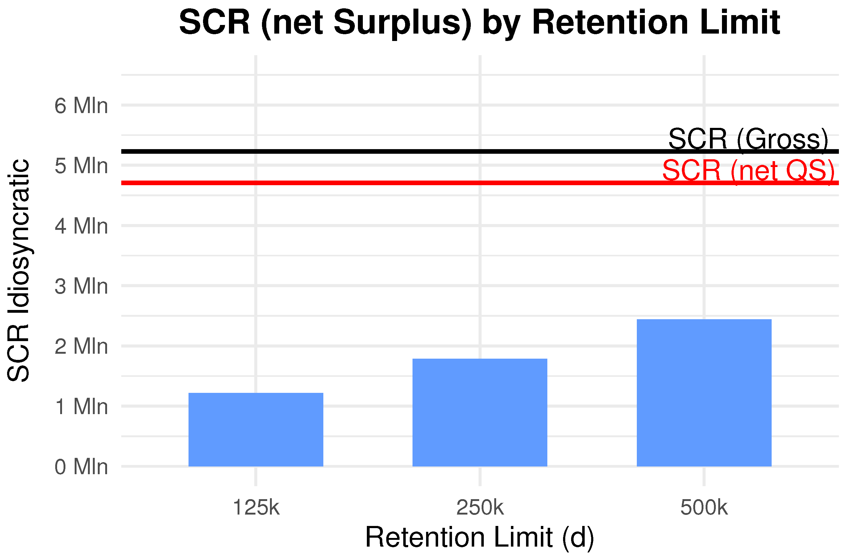
In Figure 2, we assess the impact of varying the retention limit d under Surplus reinsurance. Using the base scenario where the CV of the insured sums is 2, we explore three distinct values of d: EUR 125,000, EUR 250,000, and EUR 500,000. These values correspond to the 79%, 91.5%, and 97.2% quantiles of the sums insured distribution, respectively. As a result, the average value of the retention percentage, α k , within the portfolio is 90%, 96.7%, and 99% for each corresponding value of d.
In the scenario where d = 125,000 (i.e., the first case), the average retention percentage α k is equal to α , and the insurance company cedes approximately 42% of its initial profit. However, the capital required under this arrangement is reduced to just 23% of the capital required in the gross case, indicating a significant reduction in the capital requirement through reinsurance.
Conversely, in the case where d = 500,000, only 3% of the contracts are partially ceded to the reinsurer, but the cap on the most extreme insured sums effectively reduces the capital requirement by about 50%. This highlights the nuanced effect of the retention limit: while fewer contracts are ceded, limiting the retention on higher sums insured leads to a substantial reduction in capital, without significantly affecting profitability. These findings underscore the importance of calibrating the retention limit d to strike a balance between profitability and capital efficiency, depending on the risk profile of the portfolio.
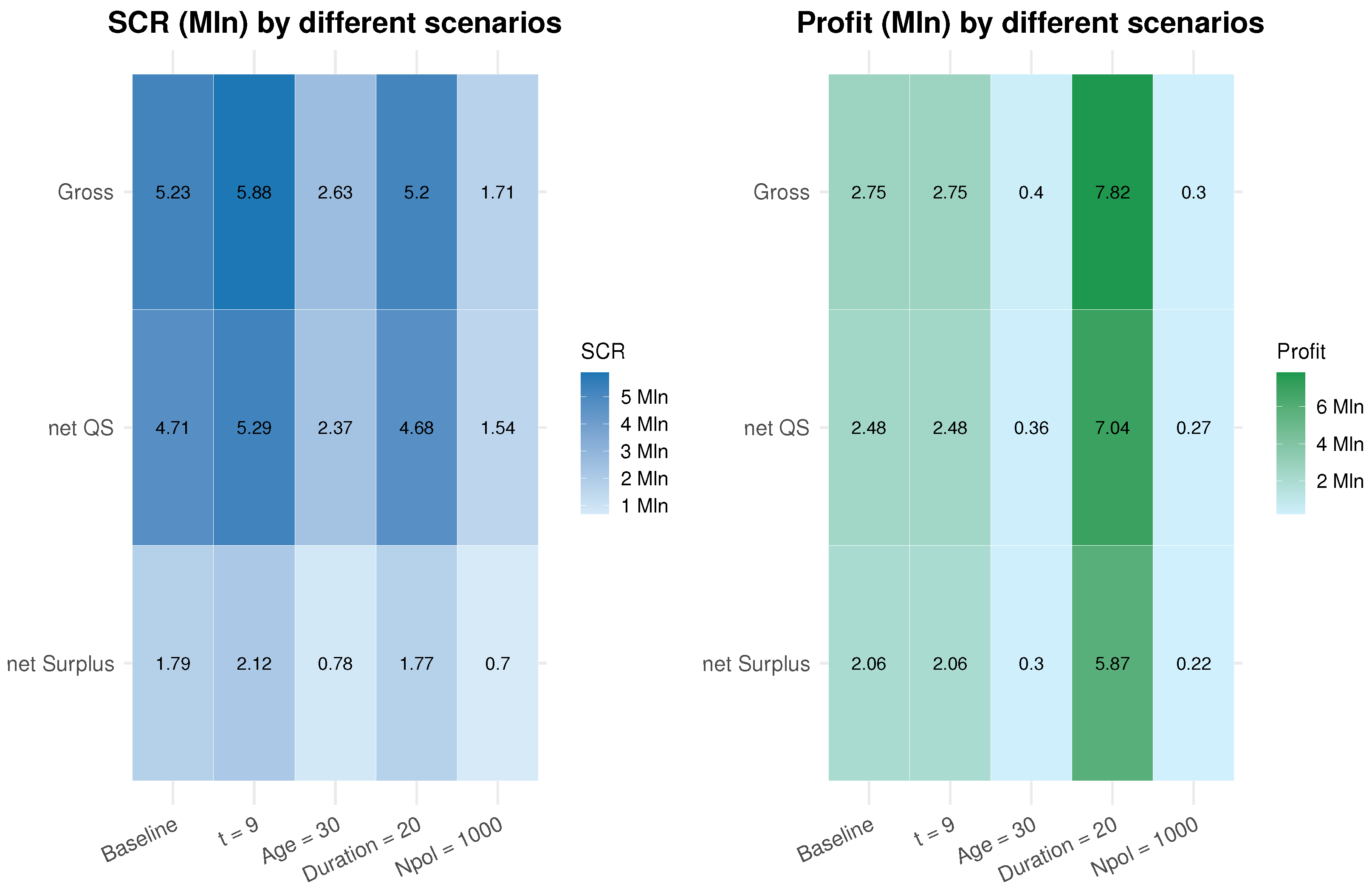
Figure 3 illustrates the impact of contract and policyholder characteristics on the SCR and profitability. Specifically, it examines how variations in the valuation time t, contract duration n, policyholder age at inception x, and initial number of policyholders l 0 influence these outcomes. When the valuation time t is varied, no effect is observed on profitability at inception, as the contract has already been underwritten. However, approaching the end of the contract term ( t = 9 ), the annual mortality risk increases due to higher Sums-at-Risk and elevated death probabilities. Regarding reinsurance strategies, the capital savings remain broadly consistent with those observed in the baseline scenario.
Younger cohorts ( x = 30 ) are associated with lower mortality probabilities and lower Best Estimate rates. As a result, profitability at inception is reduced. The corresponding CDR distribution exhibits lower variability but increased skewness. Consequently, the required capital is lower; however, the impact of Surplus reinsurance becomes more pronounced.
In contrast, a longer contract duration ( n = 20 ) has a more substantial impact on profitability. While the required capital remains nearly unchanged, profitability at inception increases significantly due to a higher Best Estimate rate. Reinsurance strategies yield results that are broadly consistent with those observed in the baseline scenario.
Finally, when the size of the cohort is reduced ( l 0 = 1000 ), both capital and profit decrease. However, while the reduction in profit is approximately proportional to the decrease in cohort size, the reduction in capital is less than proportional. Specifically, when the cohort size is reduced by a factor of ten, the standard deviation of the CDR, and thus the SCR, decreases by approximately the square root of 10. The effect of Surplus reinsurance also becomes more pronounced in this case, due to the higher skewness associated with a smaller portfolio.
In Figure 4, we examine the impact of varying the reinsurance commission rate c R E on capital requirements and profitability. Specifically, we consider the effects of more aggressive pricing by the reinsurer, achieved by reducing c R E to 0.9 and 0.8, respectively. The overall effect on capital is minimal, with a slight reduction in the required capital as c R E decreases. Lower commission rates imply a lower cash inflow for the insurer, which, in turn, leads to higher values of the net Best Estimate rates β t + 1 Q S and β t + 1 S U (see Formulas (29) and (35)). As a result, the cedent faces a reduced Sum-at-Risk in both cases, leading to a modest decrease in capital requirements.
However, the more pronounced impact is observed on profitability. For the Quota-Share treaty, the reduction in profitability increases as the commission rate decreases, with reductions ranging from 10% to 17% and 24%, respectively. Similarly, for the Surplus treaty, profitability declines more significantly, with reductions ranging from 25% to 31% and 37%. This highlights the trade-off between pricing aggressiveness and profitability, where a lower commission rate leads to reduced cedent profitability without a substantial impact on capital. In conclusion, while changes in the commission rate have a limited effect on capital, they significantly influence profitability, especially under more aggressive pricing scenarios.
In order to provide a more detailed analysis of the pricing rule established by the reinsurer and to improve the comparability between different treaties, we examine an additional scenario in which the reinsurer sets the price based on the reduction in risk for the cedent company as a result of the treaty. Specifically, we explore two alternative approaches.
In the first case, we define the commission rate as:
c r e = V a r P C D R t + 1 Idios , net | F t V a r P C D R t + 1 Idios | F t
where Var P C D R t + 1 Idios | F t represents the variance of the CDR gross of reinsurance, as defined in Equation (24), while Var P C D R t + 1 Idios , net | F t is the variance computed net of reinsurance (whether quota share or surplus, depending on the specific case analyzed). The commission rate specified in Equation (36) is proportional to the risk retained by the company. In the absence of reinsurance, c r e = 1 , whereas the commission rate decreases as the proportion of risk ceded increases.
In the second approach, the reinsurer sets c r e = 1 but introduces an additional annual loading in the premium rate based on the volatility retained. Specifically, the total premium paid to the reinsurer for the entire portfolio is increased by an additional amount l r e , which is defined as:
l r e = δ · V a r P C D R t + 1 Idios | F t V a r P C D R t + 1 Idios , net | F t
where δ is the percentage of the ceded risk that is incorporated into the pricing structure.
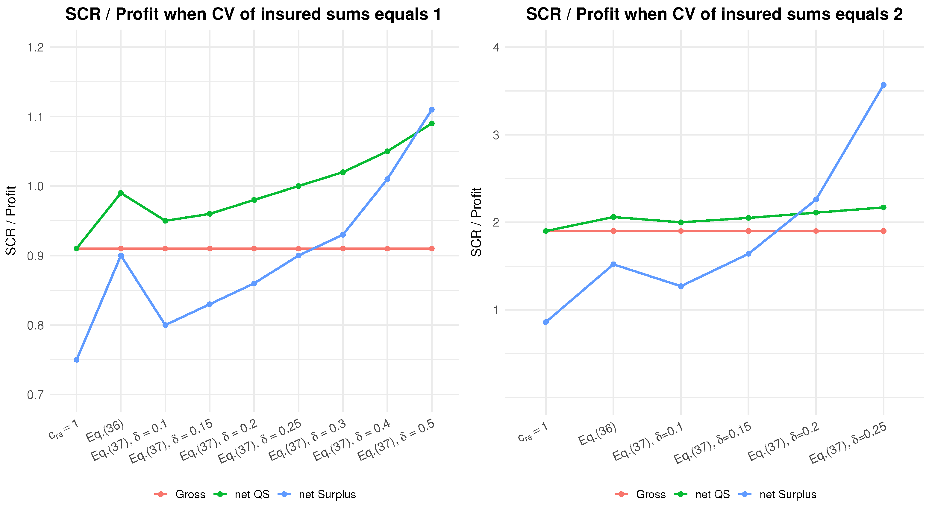
We present in Figure 5 the effects of both approaches, considering quota-share and surplus treaties, while varying the parameter δ . The analysis is conducted for both the baseline scenario and the scenario in which the coefficient of variation of the insured sum is equal to 1. Since an increase in the reinsurance price leads to a reduction in capital relief and profitability at time 0, we assess the joint effect by displaying, in the figure, the ratio between the SCR at time t for idiosyncratic risk and the profit realized at time 0. In other words, the proposed indicator can be interpreted as a capital-to-profit ratio reflecting the amount of capital required to generate one unit of profit.
When there is no variability in the insured sums within the portfolio, the capital-to-profit ratio remains the same for both gross and net of reinsurance, regardless of whether a quota-share or surplus treaty is used. As shown in Section 7.1, the two treaties behave identically, producing the same reduction in SCR and profitability, which corresponds to the portion ceded to the reinsurer. When maintaining a commission rate of 1 but increasing the coefficient of variation of the insured sums to 1, the capital-to-profit ratio increases (from 0.61 to 0.91 in the gross case). As shown in Figure 5, while the quota-share treaty again yields the same result as the gross case, a lower ratio is observed for the surplus treaty, emphasizing the benefits provided by this type of reinsurance.
The other scenarios presented in the figure illustrate the outcomes when the pricing rule is calibrated based on the reduction in variability due to the treaty. In these scenarios, the commission rate in the first approach (Formula (36)) and the loading in the second approach (Formula (37)) differ between quota-share and surplus treaties, with the surplus case exhibiting a higher reinsurance price. In terms of the capital-to-profit ratio, the quota-share treaty becomes less advantageous compared to the gross case due to the unfavorable reinsurance price, which results in a larger reduction in profit relative to the SCR. In contrast, when a commission rate is applied, the surplus treaty outperforms the gross case. However, when a pricing rule based on volatility is introduced, the choice of δ becomes a critical factor. Specifically, for higher values of δ , the surplus treaty tends to underperform the quota-share treaty. Despite offering greater capital relief, the high reinsurance price significantly depresses profitability. It is also interesting to note that when the portfolio exhibits greater heterogeneity in the insured sums (see Figure 5, right panel), two key observations emerge. First, a higher capital-to-profit ratio is observed, along with a more significant reduction in SCR for the surplus treaty when the reinsurer sets a fair price (i.e., c r e = 1 ). Second, for lower values of δ , the surplus treaty tends to perform worse than the quota-share treaty.
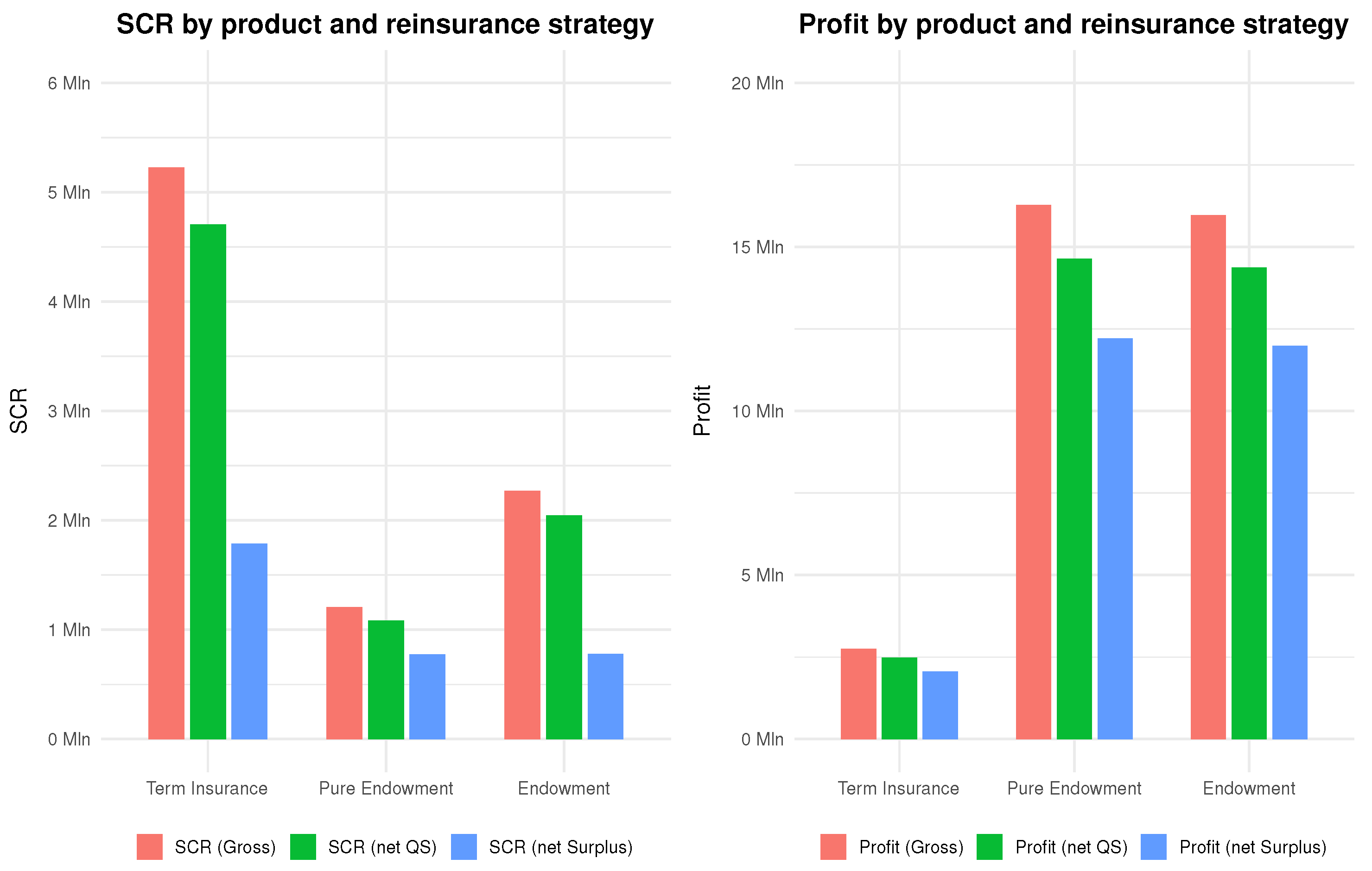
In Figure 6, we analyze the impact of the previously discussed risk mitigation strategies across different types of insurance contracts. Specifically, we compare the term insurance used in the baseline scenario with a pure endowment and a standard endowment policy. All three portfolios are assumed to consist of the same group of policyholders and to share the same distribution of sums insured. Moreover, the contracts are priced using consistent actuarial assumptions (see Table 2). The key distinction lies in the demographic assumptions adopted: for the term insurance and endowment contracts, the insurer uses a mortality table based on second-order mortality rates increased by 10%, reflecting a conservative stance toward mortality risk. Conversely, for the pure endowment contract, being exposed to longevity rather than mortality risk, a mortality table based on second-order rates reduced by 10% is applied. This approach ensures a comparable level of prudence in premium calculation while appropriately accounting for the specific risk profile of each contract.
Focusing on the gross case, the endowment product results in a lower SCR compared to term insurance, primarily due to its lower Sum-at-Risk rate, which reduces the variability of the CDR distribution according to Formula (24). A similar observation holds for the pure endowment, where the negative Sum-at-Risk rate not only lowers variability but also induces a positive skewness in the CDR distribution, further reducing the capital requirement. Additionally, both the pure endowment and endowment contracts offer higher profitability at inception, driven by a higher Best Estimate, as all contracts are priced with the same safety loading.
In the net case, we observe a consistent 10% reduction in both capital requirement and profitability across all products when a quota-share treaty is applied. In contrast, the Surplus treaty provides greater risk mitigation for products exposed to mortality risk. Specifically, term insurance and endowment show similar relative capital savings under Surplus, whereas for the pure endowment, the relative reduction is approximately half. This diminished effect is due to the already positive skewness of the CDR distribution, which limits the additional benefit provided by the Surplus treaty.

8. Conclusions

This paper introduces a modeling framework that aligns with the market-consistent valuation principles of Solvency II, offering a rigorous and adaptable approach for quantifying the idiosyncratic demographic risk in traditional insurance contracts. By focusing on a cohort of policyholders, the analysis explores the effect of proportional reinsurance on the Solvency Capital Requirement and on profitability. Although centered on a single cohort, the methodology is easily extendable to larger portfolios, making it applicable for testing the reinsurance effects in more complex settings.
A key innovation lies in the formalization of the Claims Development Result under different reinsurance structures. This allows for a detailed decomposition of demographic risk and provides closed-form expressions that incorporate reinsurance effects. Notably, the framework captures the dual impact of reinsurance: reducing capital requirements while transferring part of the expected profit to the reinsurer. This trade-off is evaluated both analytically and numerically, providing insights from a risk management perspective.
In particular, we also show how testing alternative reinsurance pricing methodologies enables a more comprehensive comparison across different reinsurance structures, including quota-share and surplus treaties, under varying risk conditions. The numerical analysis, which includes the capital-to-profit ratio as a key indicator, reveals several important insights. Specifically, when the insured sums exhibit variability, surplus treaties generally offer better capital relief but at the cost of reduced profitability, particularly when a volatility-based pricing rule is applied with a higher multiplier of the standard deviation. The study also highlights that higher reinsurance prices can erode the benefits of surplus treaties, making quota-share treaties more advantageous in certain scenarios.
The model also accounts for heterogeneity in sums insured, a feature often overlooked in traditional models, which proves crucial in assessing both the diversifiable risk component and the reinsurance effect. Indeed, the results emphasize the critical role of pricing structures in determining reinsurance effectiveness, particularly when the portfolio exhibits greater heterogeneity in insured sums. These findings offer new insights into the trade-offs between capital relief and profitability in reinsurance pricing.
In terms of implementation, the framework is computationally efficient and compatible with matrix-based calculations (see Clemente et al. 2024b), making it suitable for integration into internal modeling systems and real-time decision-making processes.
Another important aspect is represented by the consideration of the counterparty default risk associated with reinsurance as a mitigation strategy for demographic risk. Specifically, the use of reinsurance exposes the insurance undertaking to counterparty default risk, which is an important consideration within the Solvency II framework. The Best Estimate of the liabilities ceded to the reinsurer could be used to calculate the recoverables and, consequently, the SCR for counterparty default risk under the Solvency II standard formula. Future research could focus on extending the framework to enable a comparison between the aggregated SCR (net of reinsurance) and the gross SCR, providing insight into how reinsurance impacts the overall risk profile of the insurance undertaking, not only in terms of demographic risk but also with respect to counterparty risk.
While the current focus is on assessing the reinsurance effect, the model has significant potential for further adaptation. It could be extended to account for alternative regulatory frameworks or to integrate additional risk components, such as those required for the calculation of the Risk Margin or the default risk of the reinsurance company. This would provide a more comprehensive view of the mitigation effect, enabling a thorough evaluation of technical provisions and laying the foundation for a more complete internal model.

Author Contributions

All authors contributed significantly to all stages of the work, from conceptualization to the final version. All authors have read and agreed to the published version of the manuscript.

Funding

Gian Paolo Clemente, Francesco Della Corte and Nino Savelli acknowledge funding by the European Union–Next Generation EU. Project PRIN 2022 “Building resilience to emerging risks in financial and insurance markets”. Project code: 2022FWZ2CR-CUP J53D23004560008. The views and opinions expressed are only those of the authors and do not necessarily reflect those of the European Union or the European Commission. Neither the European Union nor the European Commission can be held responsible for them.

Data Availability Statement

The original contributions presented in this study are included in the article material. Further inquiries can be directed to the corresponding author.

Conflicts of Interest

The authors declare no conflicts of interest.

Appendix A. Claims Development Result for Idiosyncratic Risk

Based on Formula (15), and under our assumptions, the expanded form of the total Best Estimate for each t 0 , , n 1 is given by:
R t = E t V a P o t X ( t ) out X ( t ) in = = k = 1 l 0 s = 0 n t 1 C k , t · E t P h = 0 s 1 I k , t + h L · I k , t + s B · B t + s + 1 out , t + k = 1 l 0 c k , 0 · γ A · 1 t = 0 · B 0 out , 0 k = 1 l 0 s = 0 n t 1 C k , t · E t P h = 0 s 1 I k , t + h L · p + γ A · B t + s in , t .
In Formula (A1), it is possible to distinguish the component of the total Best Estimate related to the pure provision, represented by the cash flows X ( t ) out : pure X ( t ) in : pure , and the component related to the expenses provision, as defined in Formula (14).
Similarly, we expand Formula (16) and rewrite it by isolating the first term in the first component (corresponding to s = 0 ) from the cross-product sums:
V t + 1 : = E t + 1 V a P o t X ( t ) out : pure X ( t + 1 ) in : pure X ( t + 1 ) in : A = = k = 1 l 0 s = 0 n t 1 C k , t · E t P h = 0 s 1 I k , t + h L · I k , t + s B · B t + s + 1 out , t + 1 k = 1 l 0 s = 1 n t 1 C k , t · E t P h = 0 s 1 I k , t + h L · p + γ A · B t + s in , t + 1 = k = 1 l 0 C k , t · E t P I k , t B · B t + 1 out , t + 1 + k = 1 l 0 C k , t · s = 1 n t 1 E t P h = 0 s 1 I k , t + h L · I k , t + s B · B t + s + 1 out , t + 1 k = 1 l 0 C k , t s = 1 n t 1 E t P h = 0 s 1 I k , t + h L · p + γ A · B t + s in , t + 1 .
We present here the expanded form of Formula (18). By expanding the terms, we factor out the summations over the number of contracts and rewrite the T t + 1 -measurable cohort sum insured at time t + 1 using its definition.
R t + 1 * : = E t + 1 V a P o t X ( t + 1 ) out X ( t + 1 ) in = = k = 1 l 0 s = 0 n t 2 C k , t + 1 · E t P h = 0 s 1 I k , t + h + 1 L · I k , t + s + 1 B · B t + s + 2 out , t + 1 k = 1 l 0 s = 0 n t 2 C k , t + 1 · E t P h = 0 s 1 I k , t + h + 1 L · p + γ A · B t + s + 1 in , t + 1 = k = 1 l 0 C k , t · I k , t L · s = 0 n t 2 E t P h = 0 s 1 I k , t + h + 1 L · I k , t + s + 1 B · B t + s + 2 out , t + 1 s = 0 n t 2 E t P h = 0 s 1 I k , t + h + 1 L · p + γ A · B t + s + 1 in , t + 1 .
Accordingly, the idiosyncratic CDR in Formula (19) may be expressed in its expanded form as follows:
C D R t + 1 Idios : = V t + 1 X t + 1 out : pure R t + 1 * = = k = 1 l 0 s = 0 n t 1 C k , t · E t P h = 0 s 1 I k , t + h L · I k , t + s B · B t + s + 1 out , t + 1 k = 1 l 0 s = 1 n t 1 C k , t · E t P h = 0 s 1 I k , t + h L · p + γ A · B t + s in , t + 1 k = 1 l 0 C k , t · I k , t B · B t + 1 out , t + 1 k = 1 l 0 s = 0 n t 2 C k , t + 1 · E t P h = 0 s 1 I k , t + h + 1 L · I k , t + s + 1 B · B t + s + 2 out , t + 1 + k = 1 l 0 s = 0 n t 2 C k , t + 1 · E t P h = 0 s 1 I k , t + h + 1 L · p + γ A · B t + s + 1 in , t + 1 .
By considering the last step in Formulas (A2) and (A3), we can rewrite the idiosyncratic CDR as follows:
C D R t + 1 Idios = k = 1 l 0 C k , t · E t P I k , t B · B t + 1 out , t + 1 + k = 1 l 0 C k , t · s = 1 n t 1 E t P h = 0 s 1 I k , t + h L · I k , t + s B · B t + s + 1 out , t + 1 s = 1 n t 1 E t P h = 0 s 1 I k , t + h L · p + γ A · B t + s in , t + 1 k = 1 l 0 C k , t · I k , t B · B t + 1 out , t + 1 k = 1 l 0 C k , t · I k , t L · s = 0 n t 2 E t P h = 0 s 1 I k , t + h + 1 L · I k , t + s + 1 B · B t + s + 2 out , t + 1 s = 0 n t 2 E t P h = 0 s 1 I k , t + h + 1 L · p + γ A · B t + s + 1 in , t + 1 .
The formula can be rewritten by noting that the first and third lines both correspond to the payment of the pure cash out at time t + 1 . Moreover, applying an index shift to the second line and setting s = 0 yields the definition of the Sum-at-Risk rate β t + 1 , given in Formula (22), which also appears in the last line. This leads to:
C D R t + 1 i d i o s = k = 1 l 0 C k , t · E t P I k , t B I k , t B · B t + 1 out , t + 1 + k = 1 l 0 C k , t · E t P I k , t L I k , t L · β t + 1 ,
where, since I k , τ 1 B = I k , τ 1 D = 1 I k , τ 1 L , we have:
C D R t + 1 i d i o s = k = 1 l 0 C k , t · E t P I k , t B I k , t B · B t + 1 out , t + 1 β t + 1 ,
which, upon setting η t + 1 = B t + 1 out , t + 1 β t + 1 , coincides with formula (21).

Appendix B. Moments of the Claims Development Result for Idiosyncratic Risk

To prove Formula (24) we define the hedgeable filtration (see Malamud et al. 2008) H t = H t t = 0 , , n 1 and H t + 1 = σ T t , G t + 1 . Then:
V a r P C D R t + 1 Idios | F t = E P V a r P C D R t + 1 Idios | H t + 1 | F t + V a R P E P C D R t + 1 Idios | H t + 1 | F t = E P V a r P C D R t + 1 Idios | H t + 1 | F t 0 .
To define the cumulants of order greater than one, we introduce the r.v. corresponding to the sum insured of deaths occurring for a generic policyholder within the period ( t , t + 1 ] , with t 0 , , n 1 ,
Z k , t B = C k , t · I k , t B ,
where C k , t is F t -measurable while I k , t B is F t + 1 -measurable.

Appendix B.1. Deterministic Parameter

We define the moment generating function (mgf) of the r.v. Z k , t B assuming I k , t B follows a Bernoulli distribution with deterministic parameter q x + t . For the moment, we disregard the uncertainty in the Bernoulli parameter.
M Z k , t ( s ) = M I k , t B ( C k , t · s ) = E t P e s · C k , t · I k , t B = 1 q x + t + q x + t · e s · C k , t .
Let Z t = k = 1 l 0 Z k , t be the r.v. representing the total sum insured of deaths occurring in the period ( t , t + 1 ] . This quantity can be interpreted as a weighted sum of Bernoulli random variables, with weights C k , t .21 Assuming that within the cohort the random variables I k , t B are conditionally i.i.d., we obtain:
M Z t ( s ) = M I k , t B k = 1 l 0 C k , t · s = k = 1 l t M I k , t B ( C k , t · s ) = k = 1 l t 1 q x + t + q x + t · e s · C k , t .
From the definition of cumulative generating function Ψ Z t ( s ) = l n M Z t ( s ) we have:
Ψ Z t ( s ) = k = 1 l t l n 1 q x + t + q x + t · e s · C k , t .
The n-th cumulant K n of Z t is given by:
K n = d n Ψ Z t ( s ) d s n s = 0 .
Hence:
E t P ( Z t ) = k = 1 l t q x + t · C k , t = l t · q x + t · C ¯ t ,
V a r t P ( Z t ) = k = 1 l t q x + t · 1 q x + t C k , t 2 = l t · q x + t · 1 q x + t · C ¯ t 2 ,
where C t ¯ j = E t P C k , t j denotes the j-th raw moment of the distribution of the sum insured at the cohort level.

Appendix B.2. Stochastic Parameter

Now we consider a Bernoulli r.v. with random parameter Q x + t , with expected value q x + t and variance σ Q x + t 2 . Since Q x + t is common to all policyholders in the cohort, when it is stochastic, it induces dependence between the individual Bernoulli variables. This dependence becomes relevant when moving from the single k-th policyholder to the aggregate portfolio, as all policyholders’ risks are then subject to the same randomness introduced by Q x + t . Consequently, the number of deaths in the portfolio no longer follows a simple sum of independent Bernoulli random variables. Instead, the aggregated loss may follow a compound or mixture distribution. The aggregate expected value is unaffected by this dependence:
E t P ( Z t ) = k = 1 l t E t P Q x + t · C k , t = l t · q x + t · C ¯ t .
Dependence does affect higher-order moments. In particular, by the law of total variance:
V a r P ( Z t ) = E P V a r P Z t | Q x + t + V a r P E P Z t | Q x + t = l t · q x + t · 1 q x + t · C ¯ t 2 + l t 2 · C ¯ t 2 · σ Q x + t 2 .

Appendix C. Claims Development Result with Reinsurance

Appendix C.1. Surplus Reinsurance

The total Best Estimate, net of Surplus reinsurance, defined by Formula (27), is expanded and presented below:
R t SU = E t V a P o t k = 1 l 0 α k · X k , ( t ) out : pure + X ( t ) out : M + X ( t ) out : A k = 1 l 0 α k · X k , ( t ) in : pure k = 1 l 0 α k + c R E · 1 α k · X k , ( t ) in : A + X k , ( t ) in : M = k = 1 l 0 s = 0 n t 1 C k , t · α k · E t P h = 0 s 1 I k , t + h L · I k , t + s B · B t + s + 1 out , t + k = 1 l 0 s = 0 n t 1 C k , t · E t P h = 0 s 1 I k , t + h L · γ M · B t + s out , t + k = 1 l 0 c k , 0 · γ A · 1 t = 0 · B 0 out , 0 k = 1 l 0 s = 0 n t 1 C k , t · α k · E t P h = 0 s 1 I k , t + h L · p + 1 + c R E · 1 α k α k · ( γ A + γ M ) · B s in , t .
We denote by V t + 1 SU the available amount at the beginning of the year t, expressed in terms of its value at time t + 1 , under Surplus reinsurance:
V t + 1 SU : = E t + 1 V a P o t k = 1 l 0 α k · X k , ( t ) out : pure + k = 1 l 0 X k , ( t + 1 ) out : M k = 1 l 0 α k · X k , ( t + 1 ) in : pure k = 1 l 0 α k + c R E · 1 α k · X k , ( t + 1 ) in : A + X k , ( t + 1 ) in : M = k = 1 l 0 s = 0 n t 1 C k , t · α k · E t P h = 0 s 1 I k , t + h L · I k , t + s B · B t + s + 1 out , t + 1 + k = 1 l 0 s = 1 n t 1 C k , t · α k · E t P h = 0 s 1 I k , t + h L · γ M α k · B t + s out , t + 1 k = 1 l 0 s = 1 n t 1 C k , t · α k · E t P h = 0 s 1 I k , t + h L · p + 1 + c R E · 1 α k α k · ( γ A + γ M ) · B t + s in , t + 1 .
We denote by R t + 1 SU , * the total Best Estimate at time t + 1 , net of Surplus reinsurance, conditional on the demographic assumptions established at time t remaining valid.
R t + 1 SU , * = E t + 1 V a P o t k = 1 l 0 α k · X k , ( t + 1 ) out : pure + X ( t + 1 ) out : M k = 1 l 0 α k · X k , ( t + 1 ) in : pure k = 1 l 0 α k + c R E · 1 α k · X k , ( t + 1 ) in : A + X k , ( t + 1 ) in : M = k = 1 l 0 s = 0 n t 2 C k , t + 1 · α k · E t P h = 0 s 1 I k , t + h + 1 L · I k , t + s + 1 B · B t + s + 2 out , t + 1 + E t P h = 0 s 1 I k , t + h + 1 L · γ M α k · B t + s + 1 out , t + 1 k = 1 l 0 s = 0 n t 2 C k , t + 1 · α k · E t P h = 0 s 1 I k , t + h + 1 L · p + 1 + c R E · 1 α k α k · ( γ A + γ M ) · B t + s + 1 in , t + 1 .
Following the methodology detailed in Appendix A, we explicitly express C D R t + 1 Idios , SU as follows:
C D R t + 1 Idios , SU = k = 1 l 0 C k , t · α k · E t P I k , t B · B t + 1 out , t + 1 + k = 1 l 0 s = 1 n t 1 C k , t · α k · E t P h = 0 s 1 I k , t + h L · I k , t + s B · B t + s + 1 out , t + 1 + k = 1 l 0 s = 1 n t 1 C k , t · α k · E t P h = 0 s 1 I k , t + h L · γ M α k · B t + s out , t + 1 k = 1 l 0 s = 1 n t 1 C k , t · α k · E t P h = 0 s 1 I k , t + h L · p + 1 + c R E · 1 α k α k · ( γ A + γ M ) · B t + s in , t + 1 k = 1 l 0 C k , t · α k · I k , t B · B t + 1 out , t + 1 k = 1 l 0 C k , t · α k · I k , t L · { s = 0 n t 2 E t P h = 0 s 1 I k , t + h + 1 L · I k , t + s + 1 B · B t + s + 2 out , t + 1 + s = 0 n t 2 E t P h = 0 s 1 I k , t + h + 1 L · γ M α k · B t + s + 1 out , t + 1 s = 0 n t 2 E t P h = 0 s 1 I k , t + h + 1 L · p + 1 + c R E · 1 α k α k · ( γ A + γ M ) · B t + s + 1 in , t + 1 } .
With the same steps highlighted in Appendix A, we obtain the following compact formula, which coincides with Formula (28):
C D R t + 1 Idios , SU = k = 1 l 0 C k , t · α k · E t P I k , t B I k , t B · η t + 1 SU .

Appendix C.2. Quota-Share Reinsurance

Analogously to the Surplus case, the corresponding quantity under a Quota-Share treaty can be expressed. The total Best Estimate, net of Quota-Share reinsurance and defined in Formula (33), is presented below in its expanded form:
R t QS = E t V a P o t α · X ( t ) out : pure + X ( t ) out : M + X ( t ) out : A α · X ( t ) in : pure α + c R E · 1 α · X ( t ) in : A + X ( t ) in : M = α · { k = 1 l 0 s = 0 n t 1 C k , t · E t P h = 0 s 1 I k , t + h L · I k , t + s B · B t + s + 1 out , t + k = 1 l 0 s = 0 n t 1 C k , t · E t P h = 0 s 1 I k , t + h L · γ M α · B t + s out , t + k = 1 l 0 c k , 0 · γ A α · 1 t = 0 · B 0 out , 0 k = 1 l 0 s = 0 n t 1 C k , t · E t P h = 0 s 1 I k , t + h L · p + 1 + c R E · 1 α α · ( γ A + γ M ) · B t + s in , t } .
The total available amount V t + 1 QS is equal to:
V t + 1 QS : = α · { k = 1 l 0 s = 0 n t 1 C k , t · E t P h = 0 s 1 I k , t + h L · I k , t + s B · B t + s + 1 out , t + 1 + k = 1 l 0 s = 1 n t 1 C k , t · E t P h = 0 s 1 I k , t + h L · γ M α · B t + s o u t , t + 1 k = 1 l 0 s = 1 n t 1 C k , t · E t P h = 0 s 1 I k , t + h L · p + 1 + c R E · 1 α α · ( γ A + γ M ) · B t + s in , t + 1 } .
The total Best Estimate R t + 1 QS , * at time t + 1 under Quota-Share reinsurance, assuming demographic assumptions from time t remain valid is expanded as follows:
R t + 1 QS , * = E t + 1 V a P o t α · X ( t + 1 ) out : pure + X ( t + 1 ) out : M α · X ( t + 1 ) in : pure α + c R E · 1 α · X ( t + 1 ) in : A + X ( t + 1 ) in : M = α · { k = 1 l 0 s = 0 n t 2 C k , t + 1 · E t P h = 0 s 1 I k , t + h + 1 L · I k , t + s + 1 B · B t + s + 2 out , t + 1 + k = 1 l 0 s = 0 n t 2 C k , t + 1 · E t P h = 0 s 1 I k , t + h + 1 L · γ M α · B t + s + 1 out , t + 1 k = 1 l 0 s = 0 n t 2 C k , t + 1 · E t P h = 0 s 1 I k , t + h + 1 L · p + 1 + c R E · 1 α α · ( γ A + γ M ) · B t + s + 1 in , t + 1 } .
Hence, both the expanded and compact expressions for C D R t + 1 Idios , QS are derived as follows:
C D R t + 1 Idios , QS = α · { k = 1 l 0 C k , t · E t P I k , t B · B t + 1 out , t + 1 + k = 1 l 0 s = 1 n t 1 C k , t · E t P h = 0 s 1 I k , t + h L · I k , t + s B · B t + s + 1 out , t + 1 + k = 1 l 0 s = 1 n t 1 C k , t · E t P h = 0 s 1 I k , t + h L · γ M α · B t + s out , t + 1 k = 1 l 0 s = 1 n t 1 C k , t · E t P h = 0 s 1 I k , t + h L · p + 1 + c R E · 1 α α · ( γ A + γ M ) · B t + s in , t + 1 k = 1 l 0 C k , t · I k , t B · B t + 1 out , t + 1 k = 1 l 0 C k , t · I k , t L · { s = 0 n t 2 E t P h = 0 s 1 I k , t + h + 1 L · I k , t + s + 1 B · B t + s + 2 out , t + 1 + s = 0 n t 2 E t P h = 0 s 1 I k , t + h + 1 L · γ M α · B t + s + 1 out , t + 1 s = 0 n t 2 E t P h = 0 s 1 I k , t + h + 1 L · p + 1 + c R E · 1 α α · ( γ A + γ M ) · B t + s + 1 in , t + 1 } } ,
and, in its compact form,
C D R t + 1 Idios , QS = k = 1 l 0 C k , t · α · E t P I k , t B I k , t B · η t + 1 QS .
This coincides with Formula (34). The proof follows analogously to the cases of gross reinsurance and net Surplus reinsurance.

Notes

1
Random variables are indicated with capital letters, deterministic values with lowercase letters, and vectors and matrices in bold.
2
This notation is taken from (Wüthrich et al. 2010).
3
The superscript L in I k , τ L stands for Life.
4
From now on, the superscripts M and A will refer to management and acquisition, respectively.
5
Details on how the expense loadings are determined are provided in Section 4.
6
We clarify that 1 t = 0 is a function taking the value 1 if t = 0 , and 0 otherwise.
7
By contrast, for an endowment policy we should distinguish the two cases: for τ 0 , , n 1 it takes values I k , τ 1 B = I k , τ 1 D , while for τ = n , it is equal to 1.
8
The superscripts B, D in I k , τ 1 B and I k , τ 1 D stand, respectively, for benefit and death.
9
With second-order assumptions or second-order technical bases we refer to the expected realizations, without any prudence included in the valuation. They do not contain any margin and consist of the Best Estimate with respect to the insured population, often called experience basis (see, e.g., Bowers et al. 1997; Olivieri and Pitacco 2015).
10
The same relation holds for I k , τ 1 L , which, for each τ 1 , , n , are i.i.d. Bernoulli random variables described by a T τ -measurable random parameter 1 Q x + τ 1 , with expected value equal to the second-order annual survival probability, 1 q x + τ 1 , of a policyholder aged x at inception.
11
The deflator is defined as the ratio between first-order and second-order annual probabilities.
12
In the definition of the Cohort VaPo protected in Formula (13), the value of financial instruments is determined using the market-consistent accounting principle E .
13
These formulas apply to a cohort with constant annual premiums over the duration of the contract.
14
The superscript E in R t E stands for expenses.
15
Under local accounting principles R t is also referred to as the Zillmer Reserve.
16
According to Solvency II, the Best Estimate includes all future cash inflows and outflows.
17
By “predefined”, we mean either that the sum insured is determined in advance or that the mechanism governing the evolution of benefits is clearly specified.
18
An expanded version of Formula (27) is provided in Appendix C.1.
19
The expanded version of Formula (33) is provided in Appendix C.2.
20
A detailed description of the procedure used for obtaining the C D R t + 1 Idios , QS is provided in Appendix C.2.
21
Because C k , t may differ for each policyholder in the cohort, the mgf of Z t cannot be modeled as a binomial distribution without oversimplifying the variability in the sum insured.

References

  1. Albrecher, Hansjörg, Jan Beirlant, and Jozef L. Teugels. 2017. Reinsurance: Actuarial and Statistical Aspects. Hoboken: John Wiley & Sons. [Google Scholar]
  2. Bacinello, Anna Rita. 2001. Fair Pricing of Life Insurance Participating Policies with a Minimum Interest Rate Guaranteed. ASTIN Bulletin: The Journal of the IAA 31: 275–97. [Google Scholar] [CrossRef]
  3. Barigou, Karim, and Łukasz Delong. 2022. Pricing Equity-Linked Life Insurance Contracts with Multiple Risk Factors by Neural Networks. Journal of Computational and Applied Mathematics 404: 113922. [Google Scholar] [CrossRef]
  4. Barigou, Karim, Ze Chen, and Jan Dhaene. 2019. Fair Dynamic Valuation of Insurance Liabilities: Merging Actuarial Judgement with Market- and Time-Consistency. Insurance: Mathematics and Economics 88: 19–29. [Google Scholar] [CrossRef]
  5. Besson, Jean-Luc, Michel M. Dacorogna, Paolo de Martin, Michael Kastenholz, and Michael Moller. 2009. How Much Capital Does a Reinsurance Need? The Geneva Papers on Risk and Insurance—Issues and Practice 34: 159–74. [Google Scholar] [CrossRef]
  6. Bowers, Newton L., Hans U. Gerber, James C. Hickman, Donald A. Jones, and Cecil J. Nesbitt. 1997. Actuarial Mathematics, 2nd ed. Schaumburg: Society of Actuaries. [Google Scholar]
  7. Brennan, Michael J., and Eduardo S. Schwartz. 1976. The Pricing of Equity-Linked Life Insurance Policies with an Asset Value Guarantee. Journal of Financial Economics 3: 195–213. [Google Scholar] [CrossRef]
  8. Brennan, Michael J., and Eduardo S. Schwartz. 1979. Alternative Investment Strategies for the Issuers of Equity-Linked Life Insurance Policies with an Asset Value Guarantee. Journal of Business 52: 63–93. [Google Scholar] [CrossRef]
  9. Brouhns, Natacha, Michel Denuit, and Jeroen K. Vermunt. 2002. A Poisson Log-Bilinear Regression Approach to the Construction of Projected Life Tables. Insurance: Mathematics and Economics 31: 373–93. [Google Scholar]
  10. Chi, Yichun, X. Sheldon Lin, and Ken Seng Tan. 2017. Optimal Reinsurance under the Risk-Adjusted Value of an Insurer’s Liability and an Economic Reinsurance Premium Principle. North American Actuarial Journal 21: 417–32. [Google Scholar] [CrossRef]
  11. Clemente, Gian Paolo, Francesco Della Corte, and Nino Savelli. 2022. A Stochastic Model for Capital Requirement Assessment for Mortality and Longevity Risk, Focusing on Idiosyncratic and Trend Components. Annals of Actuarial Science 16: 527–46. [Google Scholar] [CrossRef]
  12. Clemente, Gian Paolo, Francesco Della Corte, and Nino Savelli. 2024a. An Undertaking-Specific Approach to Address Diversifiable Demographic Risk within the Solvency II Framework. Decisions in Economics and Finance. [Google Scholar] [CrossRef]
  13. Clemente, Gian Paolo, Francesco Della Corte, Nino Savelli, and Diego Zappa. 2024b. Market-Consistent Valuation and Capital Assessment for Demographic Risk in Life Insurance: A Cohort Approach. North American Actuarial Journal 29: 1–25. [Google Scholar] [CrossRef]
  14. Dacorogna, Michel. 2018. A Change of Paradigm for the Insurance Industry. Annals of Actuarial Science 12: 211–32. [Google Scholar] [CrossRef]
  15. Deelstra, Griselda, Pierre Devolder, Kossi Gnameho, and Peter Hieber. 2020. Valuation of Hybrid Financial and Actuarial Products in Life Insurance by a Novel Three-Step Method. ASTIN Bulletin: The Journal of the IAA 50: 709–42. [Google Scholar] [CrossRef]
  16. European Parliament and Council. 2009. Directive 2009/138/EC of the European Parliament and of the Council of 25 November 2009 on the Taking-Up and Pursuit of the Business of Insurance and Reinsurance (Solvency II). Official Journal of the European Union. Available online: https://eur-lex.europa.eu/eli/dir/2009/138/oj/eng (accessed on 20 September 2025).
  17. European Parliament and Council. 2014. Commission Delegated Regulation (EU) 2015/35. Luxembourg: European Parliament and Council. [Google Scholar]
  18. Hanbali, Hamza, Michel Denuit, Jan Dhaene, and Julien Trufin. 2019. A Dynamic Equivalence Principle for Systematic Longevity Risk Management. Insurance: Mathematics and Economics 86: 158–67. [Google Scholar]
  19. Lee, Ronald. 2000. The Lee–Carter Method for Forecasting Mortality, with Various Extensions and Applications. North American Actuarial Journal 4: 80–91. [Google Scholar] [CrossRef]
  20. Malamud, Semyon, Eugene Trubowitz, and Mario V. Wüthrich. 2008. Market-Consistent Pricing of Insurance Products. ASTIN Bulletin: The Journal of the IAA 38: 483–526. [Google Scholar] [CrossRef]
  21. Meyricke, Ramona, and Michael Sherris. 2014. Longevity Risk, Cost of Capital and Hedging for Life Insurers under Solvency II. Insurance: Mathematics and Economics 55: 147–55. [Google Scholar]
  22. Milevsky, Moshe A., S. David Promislow, and Virginia R. Young. 2006. Killing the Law of Large Numbers: Mortality Risk Premiums and the Sharpe Ratio. Journal of Risk and Insurance 73: 673–86. [Google Scholar] [CrossRef]
  23. Møller, Thomas. 1998. Risk-Minimizing Hedging Strategies for Unit-Linked Life Insurance Contracts. ASTIN Bulletin: The Journal of the IAA 28: 17–47. [Google Scholar] [CrossRef]
  24. Møller, Thomas. 2002. On Valuation and Risk Management at the Interface of Insurance and Finance. British Actuarial Journal 8: 787–827. [Google Scholar] [CrossRef]
  25. Olivieri, Annamaria, and Ermanno Pitacco. 2015. Introduction to Insurance Mathematics: Technical and Financial Features of Risk Transfers. Cham: Springer. [Google Scholar]
  26. R Core Team. 2023. R: A Language and Environment for Statistical Computing. Vienna: R Foundation for Statistical Computing. [Google Scholar]
  27. Savelli, Nino, and Gian Paolo Clemente. 2013. A Risk-Theory Model to Assess the Capital Requirement for Mortality and Longevity Risk. Journal of Interdisciplinary Mathematics 16: 397–429. [Google Scholar] [CrossRef]
  28. Villegas, Andrés M., Vladimir K. Kaishev, and Pietro Millossovich. 2018. StMoMo: An R Package for Stochastic Mortality Modeling. R Package Version 0.5.2. Journal of Statistical Software 84: 1–38. [Google Scholar] [CrossRef]
  29. Wüthrich, Mario V., Hans Bühlmann, and Hansjörg Furrer. 2010. Market-Consistent Actuarial Valuation. Cham: Springer, vol. 2. [Google Scholar]
  30. Yang, Shuai, and Kenneth Q. Zhou. 2023. On Risk Management of Mortality and Longevity Capital Requirement: A Predictive Simulation Approach. Risks 11: 206. [Google Scholar] [CrossRef]
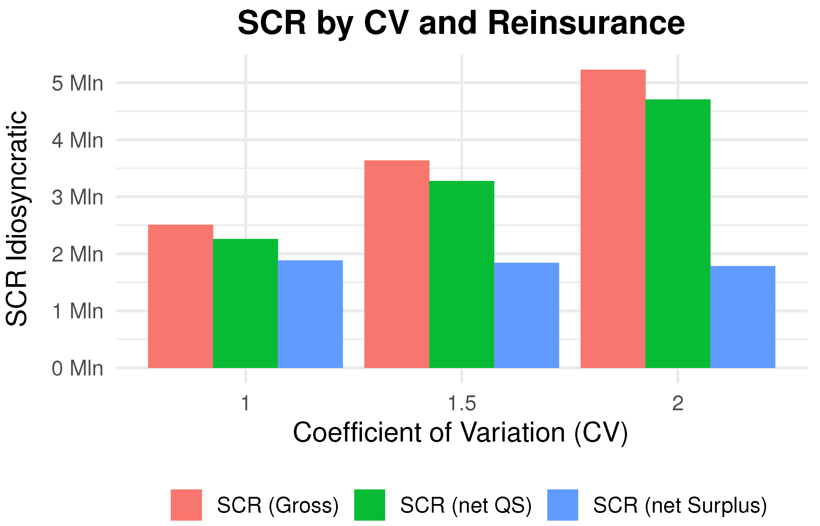
Figure 1. Solvency Capital Requirement (SCR) for idiosyncratic risk with different CV of sums insured.
Risks 13 00203 g001
Figure 2. Solvency Capital Requirement (SCR) for idiosyncratic risk with different Retention Limits.
Risks 13 00203 g002
Figure 3. Profitability at inception and Solvency Capital Requirement (SCR) for idiosyncratic risk at time t, shown relative to the gross and net cases (i.e., without and with reinsurance) across alternative scenarios. The baseline scenario considers a term insurance contract. In each alternative scenario, one of the following parameters is varied: valuation time t, contract duration n, policyholder age at inception x, or initial number of policyholders l 0 . Amounts are reported in millions of EUR.
Risks 13 00203 g003
Figure 4. Percentage reduction in profitability at inception and the Solvency Capital Requirement (SCR) for idiosyncratic risk at time t, relative to the gross (no reinsurance) case, for different proportional reinsurance treaties and varying commission rates c R E .
Risks 13 00203 g004
Figure 5. Capital-to-profit ratio (the ratio of SCR at time t for idiosyncratic risk to the initial profit) under alternative reinsurer pricing rules, where commission rate depends on the ceded risk (as defined by Formula (36) or where additional loadings are applied as a percentage δ of the ceded standard deviation (Formula (37)). Two alternative distributions of insured sums are considered, with a coefficient of variation (CV) of 1 on the left side and 2 on the right side.
Risks 13 00203 g005
Figure 6. Profitability at inception and Solvency Capital Requirement (SCR) for idiosyncratic risk at time t, shown relative to the gross and net cases (i.e., without and with reinsurance) for alternative insurance contract types. Specifically, we consider a term insurance, a pure endowment, and an endowment policy.
Risks 13 00203 g006
Table 1. Outflows and inflows at portfolio-level.
SymbolCash FlowDefinitionWhen Are They Paid?
X τ out : pure k = 1 l 0 X k , τ out : pure C k , τ 1 · I k , τ 1 B · B τ out , τ Sum insured paid out at the end of the year in which death occurs1, 2, …, n
X 0 out : A k = 1 l 0 c k , 0 · γ A · 1 t = 0 · B 0 out , 0 Anticipated acquisition expenses paid out at inception0
X τ out : M k = 1 l 0 C k , τ · γ M · B τ out , τ Anticipated management expenses paid out at the beginning of each year0, 1, …, n 1
X τ in : pure k = 1 l 0 X k , τ in : pure C k , τ · p · B τ in , τ Anticipated pure premiums collected at the beginning of each year0, 1, …, n 1
X τ in : A k = 1 l 0 X k , τ in : A C k , τ · γ A · B τ in , τ Anticipated acquisition expense loadings collected at the beginning of each year0, 1, …, n 1
X τ in : M k = 1 l 0 X k , τ in : M C k , τ · γ M · B τ in , τ Anticipated management expense loadings collected at the beginning of each year0, 1, …, n 1
Table 2. Input characteristics of the numerical analysis.
ParameterValue
Number of policyholders at inception, l 0 10,000
Average sum insured at inception, Mean c 0 100,000
Coefficient of variation of the sum insured, Std c 0 / Mean c 0 0
Cohort policyholders’ age, x50
Contract duration, n10
Valuation time, t5
Second-order demographic baseLee-Carter model, applied to data of the Italian population (age range: 0–100, time range: 2000–2021)
Risk-free rate curveEIOPA curve at the end of year 2024
First-order demographic baseSecond-order q x stressed by 10%
Technical rate2%
Acquisition expenses paid at inception as a percentage
of the insured sums, γ A
1%
Annual management expenses as a percentage
of the insured sums, γ M
0.1%
Retained percentage Quota-Share reinsurance, α 0.9
Retention limit Surplus reinsurance, d90,000
Commission rate, c R E 1
Number of simulations, M10,000,000
Table 3. Best Estimate at inception, characteristics of the simulated distributions of the Claims Development Result (CDR), and the corresponding Solvency Capital Requirement (SCR) at the end of year 5 for idiosyncratic risk, based on 10 million simulations. The SCR has been calculated under three alternative scenarios: Value at Risk (VaR) at a 99.5% confidence level, and Expected Shortfall (ES) at 99% and 99.5% confidence levels.
StatisticGross ReinsuranceNet of Quota-ShareNet of Surplus
Best Estimate at time 0−2750.62−2475.56−2475.56
Standard deviation C D R Idios 593.14534.08534.08
Skewness C D R Idios −0.20−0.20−0.20
SCR (VaR at 99.5%)1665.771499.911499.91
SCR (ES at 99%)1749.941575.701575.70
SCR (ES at 99.5%)1936.441743.621743.62
Best Estimate, standard deviation, and SCRs are in thousands of euros.
Table 4. The results pertain to the baseline scenario, where the coefficient of variation of insured sums is set to 2, and include the Best Estimate at inception, characteristics of the simulated distributions of the Claims Development Result (CDR), and the corresponding Solvency Capital Requirement (SCR) at the end of year 5 for idiosyncratic risk, based on 10 million simulations. The SCR has been calculated under three alternative scenarios: Value at Risk (VaR) at a 99.5% confidence level, and Expected Shortfall (ES) at 99% and 99.5% confidence levels.
StatisticGross ReinsuranceNet of Quota-ShareNet of Surplus
Best Estimate at time 0−2750.62−2475.56−2063.92
Standard deviation C D R Idios 1292.481164.24620.64
Skewness C D R Idios −1.39−1.39−0.34
SCR (VaR at 99.5%)5226.894706.451785.05
SCR (ES at 99%)5517.914968.491858.70
SCR (ES at 99.5%)6282.105656.582040.61
Note: Best Estimate, standard deviation, and SCRs are in thousands of euros.
Disclaimer/Publisher’s Note: The statements, opinions and data contained in all publications are solely those of the individual author(s) and contributor(s) and not of MDPI and/or the editor(s). MDPI and/or the editor(s) disclaim responsibility for any injury to people or property resulting from any ideas, methods, instructions or products referred to in the content.