Quantitative Modeling of Financial Contagion: Unraveling Market Dynamics and Bubble Detection Mechanisms

Abstract

This study explored the complex interplay and potential risk of financial contagion across major financial indices, focusing on the Bucharest Exchange Trading Investment Funds Index (BET-FI), along with global indices like the S&P 500, Nasdaq Composite (IXIC), and Dow Jones Industrial Average (DJIA). Our analysis covered an extensive period from 2012 to 2023, with a particular emphasis on Romania’s financial market. We employed Autoregressive Distributed Lag (ARDL) modeling to examine the interrelations among these indices, treating the BET-FI index as our primary variable. Our research also integrated Exponential Curve Fitting (EXCF) and Generalized Supremum Augmented Dickey–Fuller (GSADF) models to identify and scrutinize potential price bubbles in these indices. We analyzed moments of high volatility and deviations from typical market trends, influenced by diverse factors like government policies, presidential elections, tech sector performance, the COVID-19 pandemic, and geopolitical tensions, specifically the Russia–Ukraine conflict. The ARDL model revealed a stable long-term relationship among the variables, indicating their interconnectedness. Our study also highlights the significance of short-term market shifts leading to long-term equilibrium, as shown in the Error Correction Model (ECM). This suggests the existence of contagion effects, where small, short-term incidents can trigger long-term, domino-like impacts on the financial markets. Furthermore, our variance decomposition examined the evolving contributions of different factors over time, shedding light on their changing interactions and impact. The Cholesky factors demonstrated the interdependence between indices, essential for understanding financial contagion effects. Our research thus uncovered the nuanced dynamics of financial contagion, offering insights into market variations, the effectiveness of our models, and strategies for detecting financial bubbles. This study contributes valuable knowledge to the academic field and offers practical insights for investors in turbulent financial environments.

1. Introduction

In the complex landscape of global financial markets, the phenomenon of financial contagion has emerged as a critical area of investigation, influencing and shaping the interconnectedness of major indices. This research endeavors to delve into the dynamic linkages and potential contagion effects among prominent financial indices, namely the BET-FI, S&P 500, DJIA, and IXIC, with a distinctive emphasis on the unique nuances of the Romanian market. Against the backdrop of the extended timeframe spanning from 2012 to 2023, this study employed sophisticated Autoregressive Distributed Lag (ARDL) modeling methodology to meticulously dissect the complex relationships among these indices. The focal point of examination lies in the BET index, strategically chosen as the dependent variable, offering a granular perspective on the Romanian financial landscape.

Furthermore, this study integrated the Exponential Curve Fitting (EXCF) and Generalized Supremum Augmented Dickey–Fuller (GSADF) models to investigate and detect potential price bubbles formed within the analyzed indices. The analysis of financial bubbles highlights moments of heightened volatility and potential deviations from normal market trends, influenced by various governmental policies, presidential elections, the performance growth of tech companies, the COVID-19 pandemic, and the armed conflict between Russia and Ukraine.

As financial markets continue to evolve in an era of heightened global connectivity, understanding the mechanisms of contagion becomes imperative for risk assessment and effective decision-making. By elucidating the nuanced interdependencies among indices, this research not only contributes to the broader discourse on global financial contagion but also holds particular significance for the Romanian market, providing tailored insights into its susceptibility to external financial shocks. The utilization of advanced modeling techniques such as EXCF and GSADF further enhances the study’s ability to uncover and comprehend unique dynamics, contributing to a comprehensive understanding of the complex financial landscape.

According to Ionescu et al. (2023), Gajurel and Dungey (2023), and Chiriță et al. (2023), financial contagion is a phenomenon wherein an occurrence or alteration in one financial market can trigger chain reactions and disseminate to other markets or economies. This can yield noteworthy ramifications for financial and economic stability. In other words, disruptions or changes in one part of the financial market or economy can have a significant and widespread impact on other markets or sectors, denoting the effect of financial contagion. It is a form of transmission of financial shocks, where events in one country, region, or sector spread rapidly and affect other markets, creating a domino effect.

Analysis of the Romanian stock market has been approached by several researchers with the aim of trying to correlate how certain financial disruptions in the market can create systemic risk events that may manifest as financial contagion. Additionally, the ways in which other stock markets can influence the Romanian market have been examined. For instance, in the research of Davidescu et al. (2023), the effect of financial contagion was analyzed using a Dynamic Conditional Correlation Model. The authors’ findings highlighted that the stock markets of the USA and Germany influence the emerging stock markets of Central and Eastern Europe. There is also a strong link between the dynamics of macroeconomic factors and the evolution of the stock market. For example, Balint and Derecichei (2023) analyzed how the Bucharest Stock Exchange evolves and how market capitalization is influenced by the dynamics of macroeconomic factors. Furthermore, the influence of external factors such as the COVID-19 pandemic has been studied. For example, in the study of Boldeanu et al. (2022), the impact of the pandemic on the Bucharest Stock Exchange was investigated.

The aim of this research was to shed light on the complex dynamics of financial markets and reveal potential connections and reciprocal influences among the analyzed indices. In this context, we formulated several research hypotheses to guide our investigation. We assumed that there are significant interdependencies between the BET-FI index and the S&P 500, IXIC, and DJIA indices, which could lead to financial contagion effects. Additionally, we hypothesized that a detailed analysis of price movements would allow for the identification of financial bubbles, aiding in the understanding of risks and behavioral changes in markets. The primary objective of this study was to assess potential financial contagion effects among these indices and identify causal relationships by detecting price bubbles. Thus, our hypotheses can be formulated as follows:

• RQ1: There is a reciprocal influence between the BET-FI index and the international indices S&P 500, IXIC, and DJIA.
• RQ2: Detecting potential financial contagion effects among these indices highlights how events in one domain can impact and induce changes in other markets.
• RQ3: Identifying and analyzing price bubbles in the movements of the indices helps us understand the factors contributing to market volatility and the potential associated risks.

By selecting the BET-FI as the dependent variable, this research focused on the Romanian financial market, providing a detailed perspective on the specific dynamics of this environment. This enabled an in-depth analysis of the influences and interactions between the BET-FI and the international indices S&P 500, IXIC, and DJIA within the specific context of the Romanian market. Moreover, choosing the BET-FI as the dependent variable brings significant benefits for investors, analysts, and decision-makers in Romania, offering insights into how international events and changes can impact the local financial market. It serves as a valuable tool for anticipating risks and making informed decisions regarding investment portfolios.

This research aligns with the specifics of the Romanian financial market and can contribute to the local literature, addressing elements and factors relevant to the local context. This approach has the potential to highlight the unique features and dynamics of the Romanian market compared to other international markets. Additionally, the methods used in analyzing stock indices can be applied to international markets as well. Therefore, selecting the BET-FI as the dependent variable in the context of financial contagion analysis brings significant advantages for understanding the interactions between the Romanian market and international markets, providing valuable contributions to both the local and international scholarly literature.

This research is structured as follows: Section 2 provides information on the current state of the research. Section 3 presents the methodologies of the EXCF, GSADF, and ARDL models used in the analysis of the selected indices. Section 4 is dedicated to empirical results. This section showcases the financial bubbles detected through the EXCF and GSADF models, as well as the results of the ARDL model. Section 5 is devoted to discussions, conclusions, limitations of the study, and potential directions for future research.

2. The Stage of Knowledge in the Field

2.1. Financial Bubbles in the Context of Economic Crisis

Among the economic systems that have sparked particular interest among complexity science specialists, the financial market holds a privileged position. Financial markets, especially capital markets, can be characterized as complex adaptive systems. They consist of a large number of interdependent and interconnected agents exhibiting emergent group behaviors. These behaviors result from aggregating the individual actions of agents (Nica and Chirita 2021; Scarlat and Chiriță 2019). By combining these individual behaviors, the system can act cohesively at critical points, where significant changes occur due to the accumulation of low-intensity stimuli. These stimuli, when triggered, can propagate in the form of an avalanche. The financial market comprises a variety of specialized markets that facilitate transactions involving various types of financial assets. These markets, such as the money market, capital market, and foreign exchange market, operate relatively autonomously with their own interdependencies within the national economy. Transactions with financial assets occur on these markets, and understanding their specific operating mechanisms is essential for comprehending the financial system as a whole.

Throughout time, there have been numerous economic crises generated by various factors, with many of them originating from financial disruptions or the formation of price bubbles. When not addressed promptly, these events have turned into systemic risk events that propagated like a domino effect throughout the entire global financial–economic network.

The connection between economic crises and financial bubbles is complex and interconnected. Typically, financial bubbles can form when asset prices rapidly increase, surpassing their fundamental values. This rise is often fueled by excessive optimism, speculation, easy access to credit, or a combination of these factors. Also, in the periods leading up to crises, there can be a general sentiment of economic euphoria and a tendency to overvalue assets. This can lead to excessive speculation and investment in certain sectors, contributing to the formation of bubbles. When a financial bubble bursts, asset prices drop sharply, which can lead to significant financial losses for investors and financial institutions. This can trigger a financial crisis, as the decline in asset values impacts the solvency of banks and other financial institutions, causing massive capital withdrawals and credit reductions. Analyses of historical crises with the purpose of understanding the formation of financial bubbles have been conducted in several studies (Hashimoto et al. 2020; Frehen et al. 2013; Michie 2022). Therefore, the following will present some significant economic crises with the aim of highlighting how understanding these historical crises can help us identify and better understand current patterns and trends in the formation of bubbles in emerging markets, such as the Romanian market.

Tulipmania represented a period of speculative frenzy that occurred in the Netherlands between 1636 and 1637 when the prices of tulip bulbs reached extremely high levels, followed by a rapid collapse (Garber 1989). This event unfolded during a period of economic growth in the Netherlands when trade and financial innovations were in full swing (McClure and Thomas 2017). Once introduced to the Netherlands, rare varieties of tulips quickly became highly popular and were regarded as a symbol of social status. Fueled by speculation and people’s desire to increase the prices of these bulbs, special exchanges emerged where individuals could buy and sell options for future tulip bulbs. In February 1637, prices began to decline rapidly, leaving many investors holding valuable assets that became nearly worthless (Garber 2001).

Another period of crisis was the Great Depression that took place between 1929 and 1933, primarily affecting the United States (Eigner and Umlauft 2015). At the heart of this crisis was the collapse of the 1929 stock market, a symbolic event of the collapse of a massive speculative bubble. This collapse generated a massive loss of wealth and triggered a general climate of economic uncertainty (Siklos 2003). However, the Great Depression cannot be reduced to a singular event; it was fueled by other profound factors as well. The fragile banking system, characterized by unit banking and the “too-big-to-fail” concept, contributed to the expansion of the crisis (Temin 2016). Additionally, an unsustainable real estate boom and heavy financial burdens on households and financial institutions further complicated the economic landscape. Accentuated economic disparities heightened social tensions and hindered a return to normalcy. Despite similarities with other crises, the political response to the Great Depression, especially in the United States, was initially marked by inaction and hesitation (Grossman and Meissner 2010; Eigner and Umlauft 2015).

According to Ashton (1996), another crisis named the Suez Crisis, which unfolded in 1956, revolved around the nationalization of the Suez Canal. A critical aspect of this crisis was its ability to create a division between the United States and Britain following their respective policy shifts in March 1956. The British viewed Nasser as a staunch enemy, believing that his plans needed to be thwarted to prevent the undermining of Britain’s position in the Middle East—a region crucial for national survival due to its oil supplies. On the other hand, the U.S. did not perceive Nasser as a threat to anything as vital. While acknowledging Nasser’s unfavorable influence in the region and his seemingly beneficial actions for the Soviet Union, the U.S. maintained a pragmatic approach to dealing with him (Moeller 2016; Ashton 1996).

The 1997 Asian Crisis was a period of severe economic instability that impacted several East Asian countries, including Indonesia, South Korea, Thailand, the Philippines, and Malaysia (Saqib 2001). Triggered by unsustainable financial practices, economic imbalances, and structural weaknesses, the crisis had a global impact, sparking fears of financial contagion. Key consequences included currency depreciation, stock market crashes, and a sudden increase in interest rates. In an attempt to manage the crisis, the International Monetary Fund (IMF) intervened with financial support, imposing stringent conditions for economic and financial reforms, including restructuring the financial sector and reducing budget deficits. The impact on the affected economies was significant, leading to painful repercussions for living standards and employment. The crisis prompted debates on the necessary reforms within the global financial system and the importance of rigorous oversight to prevent similar events in the future (Yin et al. 2023; IMF Staff 1998). The 1997 Asian Crisis represented a transformative period in the evolution of Asian economies, highlighting the need for appropriate measures to prevent and manage financial crises on a global scale.

Also, the East Asian crisis served as a crucial lesson in illustrating the effects of financial contagion (Park and Song 2001). The connection between the two primarily refers to how panic and sudden capital withdrawals in one country triggered the phenomenon in other countries in the region. In other words, financial contagion involves the rapid spread of financial and economic problems from one country to another through a chain of interconnected events. The belief that other East Asian countries could suffer from structural issues similar to those that led to the speculative attack on Thailand prompted a massive capital withdrawal. This phenomenon of the abrupt withdrawal of capital from one country and its impact on other regional economies is what we define as financial contagion in this context. Thus, the East Asian crisis illustrated how events in one country can set off chain reactions in other economies, emphasizing the complex interconnections within the global financial system.

Another significant crisis was the Russian Crisis of 1998, which marked a period of considerable economic turbulence in Russia (Akata 2023). Factors such as substantial external debt, the collapse of commodity prices, and pervasive corruption contributed to this crisis. The critical moment occurred with the abrupt devaluation of the Russian currency, the ruble, in August 1998, and the country’s inability to meet its external debts. The impact was devastating, affecting the banking sector and financial markets and resulting in a substantial increase in unemployment. The Russian government initially attempted austerity measures to stabilize the situation but later sought financial support from the International Monetary Fund, receiving international assistance to overcome the crisis. The Russian crisis brought to light economic vulnerabilities and emphasized the necessity for more robust financial management. Furthermore, it influenced Russia’s relations with the international community and prompted significant changes in the country’s economic policies. Also, the Russian Crisis is interconnected with the phenomenon of financial contagion (Dungey et al. 2006). The abrupt devaluation of the ruble was perceived as a signal of instability and uncertainty in international financial markets. This triggered concerns about the situation in other countries with emerging economies, fueling a sense of insecurity and leading to capital withdrawals from other markets. Additionally, the Russian Crisis exerted significant pressure on other currencies and emerging economies. Investors became more hesitant about exposure to markets deemed high-risk, prompting asset sales and currency depreciations in other countries. The crisis had a broader impact on global financial markets. Investors became more cautious, reevaluating their portfolios and reducing exposures to markets deemed vulnerable. This phenomenon of financial prudence spread to other regions, contributing to a climate of uncertainty globally.

A recent crisis of major significance is the Great Recession of 2007–2009, also known as the Global Financial Crisis. It was a challenging economic period primarily triggered by the U.S. housing crisis and risky financial practices. The global impact was substantial, marked by the collapse of financial markets, rising unemployment, and a decline in economic activity. Governments implemented fiscal stimulus policies, and central banks adopted monetary measures to mitigate the crisis. Long-term effects included financial reforms and extensive debates on risk management. The Great Recession stands out as one of the most impactful economic periods in recent history, shaping global economic policy (Aiyar 2012).

The study of price bubbles has long intrigued economists, leading to a wealth of literature and diverse viewpoints in this area. Wöckl’s (2019) research offers an insightful breakdown of the main research streams in bubble analysis. He first delved into theoretical models, categorizing them into rational and behavioral bubble frameworks. The second part of his study was dedicated to empirical methods for identifying rational bubbles, with a particular focus on innovative detection techniques like recursive unit root tests, fractional integration tests, and regime-switching tests. These approaches primarily utilize advanced methods in stationarity and cointegration, concentrating on asset price time series rather than fundamental factors. This strategy sidesteps the need to validate common hypotheses about rational bubbles or the accuracy of models for asset valuation. Notably, these methods can detect bubbles that collapse periodically. While there is no universal agreement on the optimal theoretical and empirical tools for studying bubbles, empirical research in this field has seen considerable advancements. Applying different bubble detection tests to the same data often yields overlapping results, yet many findings are still inconclusive, marking bubble analysis as a fertile ground for future exploration.

2.2. Current Approaches to Financial Bubbles and Financial Contagion

The stock market experiences influences from a range of factors, encompassing news data, political stability, macroeconomic elements, and unforeseen shocks (Raza et al. 2023). Studies have indicated that these diverse factors can exert a considerable impact on both stock price returns and overall market uncertainty (Nofsinger and Sias 1999). The news-based model posits that the introduction of fresh information, whether it carries a positive or negative connotation, has the potential to alter investors’ expectations, consequently influencing stock market returns.

A review of the relevant literature on financial contagion revealed two distinct approaches: one exploring the spread of financial crises and another focusing on the limitations of associated behaviors. Concepts such as viral marketing and buying decisions are integrated into the interpretation of these phenomena, and the approach specific to financial markets analyzes the impact of the spread of crises, shocks, and disruptions. In certain contexts, these cognitive perspectives can be complementary, providing a more comprehensive understanding of the phenomenon of financial contagion. The term “contagion” was introduced in 1797 by economist David Ricardo, who associated it with the sense of panic that led to the suspension of convertibility. This concept refers to the unfounded fears of the timid part of the community (Hansen 2021).

Kolb (2011), in his research, discussed the concept of financial contagion, which borrows a fundamental meaning from the field of epidemiology. The author recommended considering the significance of this concept in the very nature of the metaphor.

Another study conducted by Paskaleva and Stoykova (2021) focused on the impact of the global financial crisis of 2008 on the capital markets of ten European Union member states. The purpose of that research was to determine whether there is a contagion effect between the Bulgarian capital market and the other markets analyzed during the crisis period and whether these markets were efficient. The methods used included the Dickey–Fuller test for argumentation, the DCC-GARCH model, autoregressive (AR) models, the TGARCH model, and descriptive statistics (Paskaleva and Stoykova 2021).

Elsayed et al. (2023) employed the ARDL model to investigate dynamic co-movements and volatility spillovers between Islamic and conventional financial markets within a dual financial system. Liao and Li (2023), on the other hand, used ARDL to investigate the factors influencing systemic risks in the Chinese financial market and to explore the early identification of indicators for systemic risks.

Țilică (2021) also analyzed the financial contagion effects within distinct economic sectors of post-communist Eastern European markets, focusing on Poland, Romania, and Russia.

Also, Pascal (2020) conducted a study focusing on stability relations within Romania’s major financial markets, including capital, foreign exchange, and monetary markets. That research explored the intensity of connections among these markets, considering them as key indicators of the economy, seen as a complex, adaptive, and dynamic systems in constant flux. The analysis centered on deviations from equilibrium, identifying factors influencing these deviations. That study incorporated market evolution and estimated volatilities, revealing that currency and stock markets are most sensitive to financial shocks. These results were correlated with events, news, and market information to understand investor behavior and the impact of their decisions on markets. Due to instability in certain markets, investors shifted their finances to more reliable markets, causing imbalances.

Additionally, several studies analyzed the situation of financial markets during the 2007–2009 financial crisis, the COVID-19 pandemic, and the Russia–Ukraine War (Wang et al. 2021; Michie 2022; Boldeanu et al. 2022). For instance, Gherghina et al. (2021) conducted a study in which they analyzed the volatility of daily returns of the Romanian stock market based on the BET index, applying the GARCH model. The authors did not identify a causal link between COVID-19 variables and the BET index. A more detailed perspective was realized by Hatmanu and Cautisanu (2021). In their study, they analyzed the impact of COVID-19 on the BET index. The authors used the ARDL model to measure the impact of the pandemic on the Romanian stock market and concluded that there was a long-term negative impact on the BET index. In another study (Insaidoo et al. 2021), an assessment of the impact of the pandemic on the performance of the Ghanaian stock market was conducted using the EGARCH (Exponential Generalized Autoregressive Conditional Heteroscedasticity) model. The authors found that there was a negative relationship between the performance of Ghana’s stock returns and the pandemic that led to an increase in return volatility. Additionally, they highlighted the importance of practical interventions by the government in such contexts.

Regarding the exploration of the effects of the COVID-19 pandemic on stock market volatility, the specialized literature highlights the use of quantitative econometric methods such as the Vector Autoregressive model (Shahzad et al. 2021; Hoshikawa and Yoshimi 2021) and the GARCH model (Gherghina et al. 2021) and its variations like ECARCH, FIGARCH, and GARCH-MIDAS (Bai et al. 2021; Fakhfekh et al. 2023). Additionally, more advanced models have been employed to capture both short-term and long-term relationships and effects, such as the ARDL model (Adam et al. 2021; Javangwe and Takawira 2022; Qamruzzaman and Wei 2018; Nusair and Al-Khasawneh 2022). Among the findings of these analyses, it has been revealed that the pandemic increased the risk of a financial market crash (Z. Liu et al. 2021), unfavorable volatility spillover shocks outweighed favorable ones (Shahzad et al. 2021), there was a higher level of volatility spillover between the U.S. and Chinese equity markets during the pandemic compared to before it (Youssef et al. 2021), and government interventions led to an increase in volatility in stock markets worldwide (Zaremba et al. 2020). Another distinct approach (Contessi and De Pace 2021), considering the most commonly used models, was employed in a study that examined how market instability was propagated during the COVID-19 pandemic. The authors utilized the GSADF model, specifically designed for identifying price bubbles, and observed that in periods characterized by significant instability caused by the pandemic, it served as a means of disseminating and generating instability in stock markets (Contessi and De Pace 2021).

On the other hand, the armed conflict between Russia and Ukraine also influenced the financial market. For example, Yousaf et al. (2022) analyzed the impact of this conflict on the G20 capital markets and concluded that the stock markets in countries such as Hungary, Poland, and Slovakia recorded negative returns in the pre-event days, while countries such as France, Germany, and Romania were negatively affected in the post-invasion days. Another study (Ullah et al. 2023) highlighted the effects of the conflict between Russia and Ukraine on the Russian financial market. The authors used the TVP-VAR and Quantile VAR approaches and concluded that during the conflict period, the risk in this market increased significantly, affecting particularly the oil and gas sector, as well as financial services. Furthermore, the Russian invasion of Ukraine had global market implications. Izzeldin et al. (2023) applied the Markov-switching HAR model to volatility proxies and observed that wheat and nickel were the most affected commodities due to the prominent exporter status of the two countries. In another study (Das et al. 2023), from the perspective of the impact of this conflict, simple linear regression models were employed, and it was concluded that this conflict had a negative impact on stock returns in European markets.

Thus, we can assert that turbulence in financial markets can swiftly manifest as financial crises and even irregularly occurring catastrophes, unexpectedly surfacing about every generation. Nonlinear dynamics seek to demonstrate that these financial market phenomena are as natural as hurricanes, earthquakes, floods, revolutions, and other disturbances in nature and society. Therefore, the financial contagion phenomenon is most fittingly associated with these events in the form of a domino effect that can occur within the financial network. Financial markets, like any complex adaptive system, exhibit complex organization and nonlinear dynamics that generate instability and even chaos. These systems, with a large number of interdependent components and openness to the external environment, naturally tend to undergo change and reorganization, continually adapting their structure and internal dynamics to better withstand environmental disruptions.

Such a conception of complex adaptive systems and their turbulent behavior is gaining widespread recognition, drawing on concepts, theories, and ideas from various scientific disciplines. Our study emphasizes a novel approach that can contribute to the development of the existing literature by combining bubble detection models and utilizing the ARDL model to determine long- and short-term causality relationships, aiming to outline the dynamic landscape of the financial market surrounded by financial contagion effects.

3. Materials and Method

3.1. Methods and Techniques for Detecting Financial Bubbles

An economic bubble is characterized by a rapid increase in the market value of assets, especially their prices, followed by a sudden decrease or contraction, a phenomenon known as a bubble burst (Chiriță et al. 2023). The phenomenon of financial bubbles occurs when asset prices grow rapidly and become disproportionate to their real value. The emergence of these bubbles is often associated with abrupt changes in investor behavior, yet there is still no universally accepted explanation for the primary cause of this phenomenon (Shu et al. 2021).

According to Watanabe et al. (2007a), financial bubbles or crashes are subjects that are increasingly attracting researchers due to their dynamic behavior. Among the authors who have provided a mathematical description of financial bubbles are Johansen and Sornette (2001), who assumed that a crash occurs after the rapid growth of economic indicators, faster than an exponential function (Sornette and Andersen 2002; Johansen and Sornette 2001; Zhou and Sornette 2006). Nevertheless, it has been considered that this proposed method is useful for predicting the end of a bubble, not its beginning. Thus, (Watanabe et al. 2007b) introduced in their article a mathematical definition of bubbles and crashes based on exponential behaviors detected in systematic data analysis.

From a mathematical perspective (Sornette and Cauwels 2014), a financial bubble is defined as the positive difference between real prices and fundamental prices (reasonable values) of assets. The real price can be described by the following mathematical formula (Phillips et al. 2011):

$$p_t={\sum }_{i=1}^{\infty }\frac{E_t\left(q_{t+i}\right)}{{\left(1+r\right)}^i}+a_t$$

(1)

In Equation (1), $p_t$ represents the stock price at a given time $t$, $E_t$ represents the expected sum calculated based on valid information available at time $t$, $q_t$ represents the dividends, and $r$ represents the discount rate. In Equation (1), the rate $r$ is considered constant throughout the period. Thus, the equilibrium price or fundamental value will be obtained. The random value of the bubble that satisfies this condition is determined by $a_t$.

$$a_t=\frac{E_t\left(a_{t+1}\right)}{(1+r)}$$

(2)

In Equation (2), the equilibrium price is described. According to this equation, as confirmed in the specialized literature, there is no concept of a negative bubble from a mathematical perspective. Nevertheless, in the context of this research, we will use the concept of a negative bubble when observing the effects of a sudden decline in the analyzed markets, and the concept of a positive bubble will be employed when the price unexpectedly rises rapidly.

From the perspective of rational expectations economics (Aoki and Nikolov 2012; Martin and Ventura 2018; Michau et al. 2023; Galí 2014), the theory of rational expectations specifies that the price of an asset can be determined through the discounted cash flows it generates. Market prices are formed based on the information available to market participants and economic models relevant to the situation. According to this theory, prices are expected to align with the intrinsic value of the asset, unless there is misinformation in the market that misleads investors. When individuals buy unprofitable stocks with the intention of selling them at a higher price and making a profit in the future, this behavior leads to an increased demand for those stocks, thereby driving up their prices. This phenomenon is known as a rational price bubble. Such bubbles continue to expand until they eventually burst, disrupting all planning and forecasting efforts.

In contrast, the theory of irrational bubbles (H. Liu et al. 2012; Seidens 2018; Baker and Wurgler 2007) posits that price bubbles can occur when irrational speculators, driven by the belief that the asset’s value will keep increasing based on its past performance, artificially drive up its price. In this scenario, the market consists of individuals with limited intellectual perspectives who fail to distinguish between market value and intrinsic value, thus contributing to the formation of a bubble. Within irrational price bubbles, people do not have rational expectations regarding the future benefits and prices of goods. Investment decisions in such situations are not based on information about risk and return, and the market operates on the basis of random and psychological reactions.

3.1.1. Exponential Curve Fitting (EXCF) Method

The Exponential Curve Fitting method is a mathematical technique used to model and analyze experimental data exhibiting exponential decay behavior. Essentially, this method aims to find an exponential function that best fits the observed dataset (Perl 1960; Foss 1970; Ma et al. 2021).

The primary application of this method lies in deducing and analyzing relevant parameters of the exponential function, such as the final equilibrium value, rate constants, or other specific characteristics of the studied phenomenon. This approach can be employed in various fields (Zuo et al. 2022; Zhang et al. 2018), including biological sciences, economics, physics, or any context where data evolution can be described by exponential decay processes.

However, the choice and application of the Exponential Curve Fitting method must be tailored to the specifics of the dataset and consider the underlying nature of the process. It is crucial to consider the complexity of the data and utilize methods that provide relevant, robust, and valid results within the context of the specific research or analysis.

The initial application of the EXCF method for identifying price bubbles in financial assets was proposed by (Watanabe et al. 2007a, 2007b). This approach relies on estimating the parameters ${\omega }_1(i,T_i)$ and $P_0(i,T_i)$ through the analysis of historical data $T_i$, aiming to identify periods when prices exhibit divergence or convergence.

$$P_t-P_{t-1}=\left({\omega }_1\left(i,T_i\right)-1\right)(P_{t-1}-P_0\left(i,T_i\right)+{\epsilon }_t$$

(3)

In Equation (3), the essential parameters are estimated, where $p_t$ denotes the financial asset’s price at time $t$, and ${\epsilon }_t$ represents the error term. The expression ${\omega }_1\left(i,T_i\right)=1$ indicates a scenario in which the price of the financial asset follows a random walk pattern. This means that the price does not exhibit a directional trend but undergoes random variations over time. In such a situation, the parameter $P_0\left(i,T_i\right)$ has limited influence on the price evolution since it is mostly determined by random or unsystematic factors.

On the other hand, when ${\omega }_1\left(i,T_i\right)>1$, this signifies either a significant increase in the value of the financial asset (known as a “bubble”) or a substantial decrease that may lead to a price collapse. The value of the parameter $P_0\left(i,T_i\right)$ in this context serves as a baseline or reference for exponential divergence. When ${\omega }_1\left(i,T_i\right)<1$, this indicates that the price of the financial asset converges toward the value of the parameter $P_0\left(i,T_i\right)$. This suggests that the price does not exhibit a significant upward or downward trend but tends to approach the baseline specified by $P_0\left(i,T_i\right)$. Consequently, the exponential divergence decreases, and the price converges toward the level determined by the same parameter.

Hence, the conditions ${\omega }_1\left(i,T_i\right)=1$, ${\omega }_1\left(i,T_i\right)>1$, ${\omega }_1\left(i,T_i\right)<1$ serve as key indicators in the EXCF model, offering valuable insights into the trends and dynamics of financial asset prices based on exponential divergence and the estimated parameters $P_0\left(i,T_i\right)$ and ${\omega }_1\left(i,T_i\right)=1$.

For identifying the most suitable time interval $T_i$, an AR(p) model is initially estimated using the original data set:

$$P_t={\sum }_{j=1}^p{\varphi }_j{P}_{t-j}+{\epsilon }_t$$

(4)

After establishing the optimal time interval $T_i$, a rolling estimation method is used to detect bubbles or periods of price crashes, following the method proposed by Fantazzini (2019).

The EXCF algorithm implementation and price bubble detection were carried out by Fantazzini (2019) using the “bubble” package in R. In this context, the parameter $P_0\left(i,T_i\right)$ was assigned the first observation from the data sample for the interval $T_i$. Additionally, Equation (4) was reformulated as an AR(p) equation without an intercept, as depicted in Equation (5).

$$P_t-P_0\left(i,T_i\right)={\omega }_1\left(i,T_i\right)[P_{t-1}-P_0\left(i,T_i\right)]+{\epsilon }_t$$

(5)

The EXCF model and the bubble detection algorithm represent a valuable approach for identifying and analyzing price bubbles in financial assets. This method relies on estimating the parameters ${\omega }_1\left(i,T_i\right)$ and $P_0\left(i,T_i\right)$ using historical data and specific detection algorithms. It can contribute to understanding and assessing price trends in the context of financial markets.

3.1.2. Generalized Augmented Dickey–Fuller (GSADF) Test

Considerable attention has been given to studying rational bubbles, which are often associated with financial crises and economic recessions. A widely used theoretical framework for understanding a rapid rise in asset prices is the rational bubble model. This model is based on evaluating a rational bubble through the lens of present value theory, where the intrinsic value of the asset is determined by estimating the expected sum of future dividends discounted to their present value. A detailed approach to this model was presented by Phillips et al. (2011). Phillips et al. (2015a) proposed recursive tests that can detect evidence of explosive behavior in time series $\left\{Y_t\right\},t=1,\dots ,T$. The reason for using recursive tests is that price behavior is dominated by the bubble component. Therefore, we can directly test for the presence of bubbles in prices.

$$Y_t=\mu +\rho Y_{t-1}+{\sum }_{i=1}^p{\varphi }_{rw}^i\mathsf{\Delta }{Y}_{t-1}+{\epsilon }_t$$

(6)

Equation (6) is a mathematical representation of the Augmented Dickey–Fuller (ADF) regression (Phillips et al. 2011).

In a study conducted by Phillips et al. (2015b), hereafter referred to as PSY, they developed a test statistic to address the presence of multiple bubbles in a time series. Specifically, they focused on the scenario where the drift term is greater than 0.5, as this is considered more significant in practical applications. The test they proposed is known as the Generalized Supremum ADF (GSADF) test. This test serves as a measure to determine the presence of explosive behavior in a time series.

The GSADF test is increasingly used for identifying price bubbles. For instance, Tan and Chan (2021) analyzed in their article how the GSADF test proposed by Phillips et al. (2015a) detected and timestamped real estate bubbles in ten major cities in China.

Phillips et al.’s (2015b) approach in their research highlights effective econometric mechanisms for identifying and dating financial bubbles in real time. Simulations conducted by the authors have shown that the GSADF test significantly improves discriminatory power and leads to distinct power gains when multiple bubbles occur. They tested the model on stock market data for the S&P 500 index.

3.2. ARDL Econometric Methodology

The Autoregressive Distributed Lag model is an econometric method used to analyze long-term relationships between variables. It is a cointegration technique that aims to identify the presence of a stable long-term relationship among the analyzed variables. The ARDL model is particularly useful when examining the links between variables that may evolve over time and affect each other in the long run. Although not developed specifically for detecting financial bubbles, it is often used in broader economic and financial analyses to examine how variables evolve in the long term and interact with each other (Nica et al. 2023a, 2023b). Detecting financial bubbles typically involves performing specific analyses, applying methods for testing the existence of bubbles, and assessing their impact on financial markets.

The ARDL model variant introduced by Pesaran and Shin (1998) and Pesaran et al. (2001) functions as a cointegration approach designed to assess the existence of a long-term relationship among variables. This advanced methodology presents various advantages compared to traditional cointegration tests, including those proposed by Engle and Granger (1987), Johansen (1988), Johansen (1991), and Johansen and Juselius (1990).

Philips (2018) notes that the ARDL method is particularly advantageous compared to other techniques because it enables the analysis of cointegration relationships among variables, even when some of them are integrated at order 0 (I(0)) and others at order 1 (I(1)). Pesaran et al. (2001) highlight the use of ARDL in scenarios of mixed integration orders. Additionally, the ARDL bounds test enables the construction of an unrestricted error correction model (ECM) through a linear transformation. According to Asteriou and Hall (2015), an ECM captures the dynamics of both long-term and short-term research variables. Remarkably, empirical evidence consistently attests to the superior performance of the ARDL model. Nkoro and Uko (2016) argue that the issue of endogeneity is less relevant within the ARDL framework due to the absence of residual correlations, indicating that all variables are endogenous. The ARDL model is as follows:

$$R_t=x_0+{\sum }_{i=1}^p{y}_i{R}_{t-i}+{\sum }_{i=0}^q{z}_i{P}_{t-i}+{\epsilon }_t$$

(7)

In Equation (7), the dependent variable $R_t$ is represented as a function of its previous values and the lagged variables of the dependent vector $P_{t-i}$. The coefficients b and c denote short-term coefficients, while y and z refer to the lag numbers for $R_t$ and $P_t$. The term ${\epsilon }_t$ represents the error term.

The ARDL process involves the following steps (Nica et al. 2023a; Androniceanu et al. 2023):

(a)

Verification of data stationarity.

(b)

Selection of the optimal lag length, which involves constructing the unrestricted Vector Autoregressive (VAR) model to identify the most suitable number of lags. An inaccurate choice of the lag length may introduce bias into the outcomes, rendering them inappropriate for forecasting and making inferences.

(c)

Verification of cointegration and development of the Error Correction Model (ECM). The ARDL model was improved by incorporating the bounds test, which examines whether a combination of I(0) and I(1) variables exhibits a long-term relationship. The structure of the ARDL bounds test is delineated by Equation (8):

$$\mathsf{\Delta }{R}_t={\lambda }_0+{\sum }_{i=1}^p{\lambda }_i\mathsf{\Delta }{R}_{t-i}+{\sum }_{i=1}^q{\nu }_i\mathsf{\Delta }{P}_{t-i}+{\tau }_1{R}_{t-1}+{\tau }_2{P}_{t-1}+{\xi }_t$$

(8)

where ${\sum }_{i=1}^p{\lambda }_i\mathsf{\Delta }{R}_{t-i}+{\sum }_{i=1}^q{\nu }_i\mathsf{\Delta }{P}_{t-i}$ constitute the short-term terms and ${\tau }_1{R}_{t-1}+{\tau }_2{P}_{t-1}$ represent the long-term terms. According to Pesaran et al. (2001), if the calculated F-value is statistically significant, the subsequent step involves constructing an Error Correction Model (ECM) to analyze both long-term and short-term dynamics. The significance of the F-value is assessed in comparison to critical values established by (Pesaran et al. 2001). A dynamic ECM can be derived through a simple linear transformation of an ARDL model. This ECM integrates short-term dynamics with long-run equilibrium, preserving crucial long-term information. By doing so, it addresses issues like spurious relationships that may arise when dealing with non-stationary time series (Shrestha and Bhatta 2018). The lagged variables $R_{t-i}$ and $P_{t-i}$ from Equation (8) are replaced with the Error Correction Term (ECT) in Equation (9). The ECM is structured as follows, as outlined in Equation (9):

$$\mathsf{\Delta }{R}_t={\lambda }_0+{\sum }_{i=1}^p{\lambda }_i\mathsf{\Delta }{R}_{t-i}+{\sum }_{i=1}^q{\nu }_i\mathsf{\Delta }{P}_{t-i}+{\tau }_1{ECT}_{t-1}+{\zeta }_t$$

(9)

If $\tau$ falls within the interval [−1, 0] and holds statistical significance, this indicates that the variables are cointegrated.

(d)

Validation and conduction of stability tests.

According to (Nandy and Chattopadhyay 2019; Khalfaoui et al. 2023), a VAR model is a statistical method used to analyze and model the interdependencies among multiple time series variables. This model is commonly employed in econometrics and time series analysis, enabling researchers and analysts to assess how changes in one variable impact the other variables within the system. For instance, Ahelegbey et al. (2021) employed a Vector Autoregressive model in conjunction with a network approach to investigate the dynamics of financial contagion among countries.

The ARDL model emerges as a versatile and powerful econometric tool that proves instrumental in analyzing relationships between variables, especially in scenarios where integration orders vary. Its flexibility allows for the examination of both short-term and long-term dynamics, making it applicable to a wide range of economic and financial studies. ARDL’s utility extends to areas such as detecting cointegration, constructing error correction models, and exploring the interconnectedness of markets. Researchers leverage ARDL to unravel complex interactions, providing valuable insights into systemic risks, contagion effects, and volatility spillovers across diverse financial landscapes. The model’s adaptability and robustness make it a valuable asset in understanding and navigating the complex dynamics of economic and financial systems.

4. Results

In the dynamic world of financial markets, detecting and understanding the complex phenomenon of price bubbles poses a crucial challenge for investors, analysts, and decision-makers in the financial sector. In this context, the use of advanced models such as Exponential Curve Fitting and Generalized Supremum Augmented Dickey–Fuller becomes essential for assessing and anticipating the evolution of prices within benchmark indices like the BET-FI, DJIA, IXIC, and S&P 500. The significance of employing EXCF and GSADF in the analysis of financial indices like the BET-FI, DJIA, IXIC, and S&P 500 becomes evident amidst high volatility and rapid changes in global markets. Identifying price bubbles in these indices is vital for investors and decision-makers, providing them with the opportunity to adjust strategies and effectively manage risks.

On the other hand, the analysis of price bubble detection is complemented by the use of the ARDL model, where the BET-FI serves as the dependent variable, while the S&P 500, DJIA, and IXIC act as independent variables. The ARDL model was employed to assess the relationships between variables, interdependencies, influences, and causality, as well as the effects of financial contagion. The BET-FI, as the dependent variable, represents the BET-FI Index, reflecting the overall performance of the financial market in Romania. Modeling this variable enables an understanding of its impact and interactions with other relevant variables. Thus, the ARDL model can unveil whether and how changes in the independent variables may influence the BET-FI, highlighting connections and interdependencies among financial markets. Additionally, the ARDL model provides the opportunity to analyze both short-term and long-term relationships, allowing the identification of immediate effects and adjustments in the dependent variable’s response to changes in the independent variables. The outcomes of the ARDL model can offer valuable insights for strategic decision-making, risk management, and the development of more effective strategies within financial markets.

The data source, analysis period, and their description are presented in

Table 1. Description of variables and sources.

Variable	Acronym	Description	Source
Bucharest Exchange Trading Investment Funds Index	BET-FI	The BET-FI Index is an indicator of the overall performance of the financial market in Romania, reflecting the movement of stock prices of the most liquid companies listed on the Bucharest Stock Exchange (BVB).	Bucharest Stock Exchange (https://bvb.ro/ accessed on 20 November 2023)
Standard and Poor’s 500	S&P 500	The S&P 500 Index, also known as the S&P 500, is a stock market index representing the financial market in the United States. It reflects the performance of 500 of the largest publicly traded companies listed on American stock exchanges, providing a comprehensive overview of the U.S. capital market.	Yahoo Finance (https://finance.yahoo.com/, accessed on 20 November 2023)
Nasdaq Composite Index	IXIC	The Nasdaq Composite Index encompasses the stocks of a broad number of companies listed on the Nasdaq Stock Market in the United States. It reflects the overall trends in the technology market and the technology sector, including companies involved in information technology, biotechnology, and other related fields.	Yahoo Finance (https://finance.yahoo.com/, accessed on 20 November 2023)
Dow Jones Industrial Average	DJIA	The Dow Jones Industrial Average Index includes the stocks of 30 of the largest and most significant American companies, reflecting the overall performance of the stock market in the United States.	Yahoo Finance (https://finance.yahoo.com/, accessed on 20 November 2023)

.

The data presented in Table 1 were gathered over the period from 2012 to October 2023. Specifically, the dataset for the ARDL model covers the timespan from 2012 to 2022, while the data used for financial bubble detection extends until October 2023. For financial bubble detection, the data used were daily, preserving the actual observed values. For the ARDL model, the data were logarithmically transformed. Logarithmic transformation helps stabilize the variances across different levels of the data, according to Gustafsson and Stockhammar (2019) and Luetkepohl and Xu (2009), making the spread more consistent. This is particularly beneficial when dealing with financial time series data that may exhibit changing levels of volatility over time.

4.1. Detecting Financial Bubbles: EXCF and GSADF Models Unveiled

In the dynamic landscape of financial markets, identifying and managing risks associated with price bubbles is a critical challenge. The use of models such as Exponential Curve Fitting and Generalized Supremum Augmented Dickey–Fuller becomes paramount in understanding price movements and anticipating potential shifts in market behavior. These analytical tools are particularly relevant in the case of key financial indices such as the BET-FI, DJIA, IXIC, and S&P 500.

According to Watanabe et al. (2007a, 2007b) and Cabello Sánchez et al. (2021), EXCF makes a significant contribution to time series analysis, providing insights into market trends and volatility. By fitting exponential curves to price data, EXCF helps highlight significant patterns, facilitating the identification of potential price bubbles and the anticipation of directional changes. On the other hand, GSADF, with its robust approach, according to Peng et al. 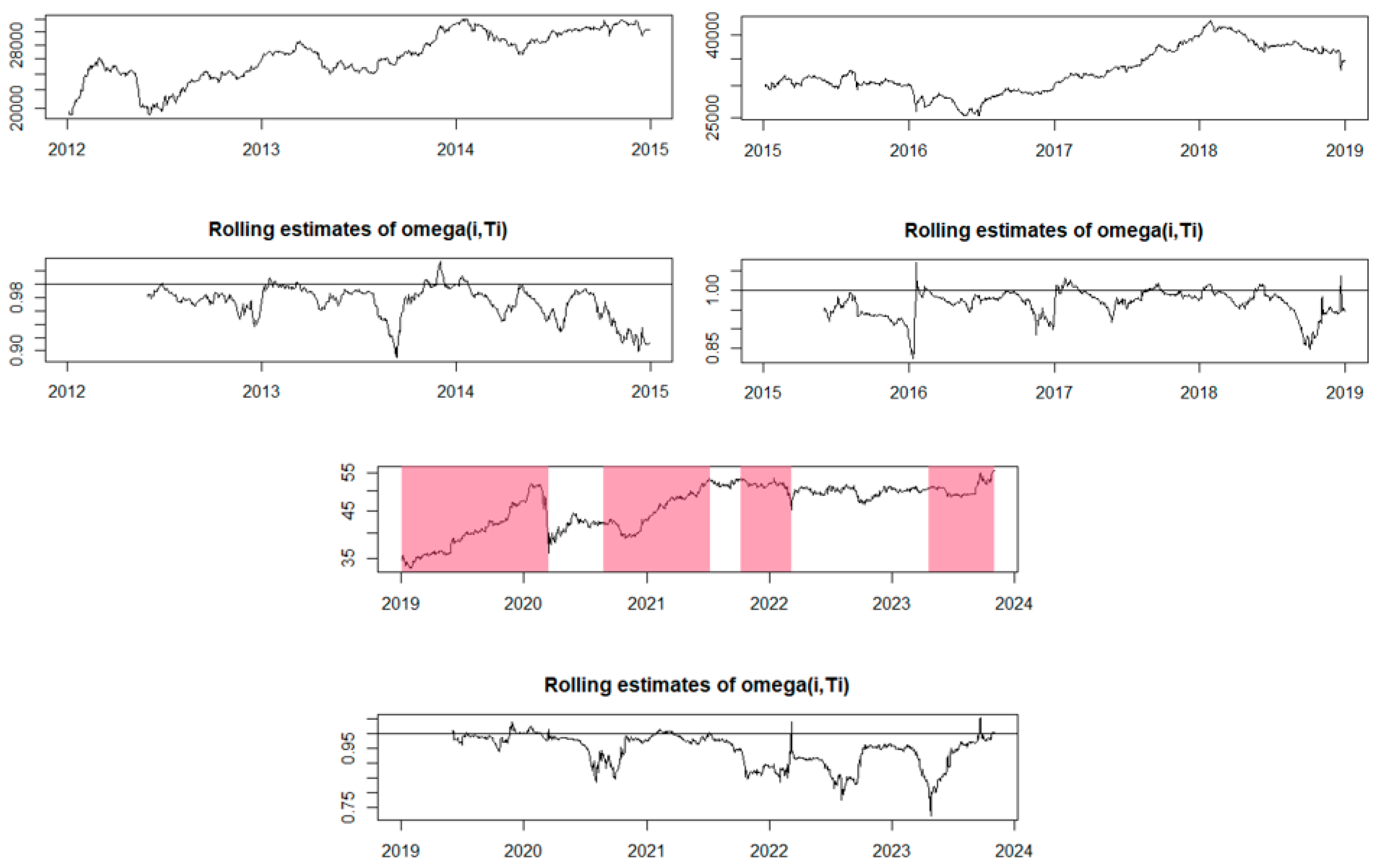(2023) explores the phenomenon of price bubbles and contributes to validating the results obtained with EXCF. By integrating this model into our analysis, we had the opportunity to confirm and strengthen warning signals, adding an additional level of confidence to the process of identifying price bubbles. The importance of this analysis extends beyond the identification and quantification of price bubbles in isolation. As financial markets are interconnected, the phenomenon of financial contagion becomes a crucial component. Identifying a bubble in a major index, such as the S&P 500, can influence the behavior of other indices, such as the BET-FI, DJIA, and IXIC. By using EXCF and GSADF to examine these interdependencies, we gain a broader and more precise view of how changes in one index can propagate and affect the entire financial landscape. The EXCF model uses rolling estimates with the aim of providing information about the variation in volatility and significant changes in the dynamics of the analyzed time series. These estimates offer insight into how volatility changes over time and can help identify periods where it increases significantly, indicating potential points of interest for the analysis of financial bubbles. The interpretation of these estimates is performed in the context of the analyzed time series. When the rolling estimates present higher values, this suggests increased volatility during those periods, which may be associated with potentially significant changes in market prices. Generally, areas with high values of the rolling estimates can draw attention to periods where there is an increased probability of the formation of financial bubbles or significant events in the market.

Through this integrated analysis, we aimed to make a significant contribution to understanding the dynamics of financial markets, allowing investors and decision-makers to approach the risks associated with price bubbles with more confidence and develop more informed strategies in the face of global market challenges.

In Figure 1, the evolution of closing prices for the analyzed indices has been depicted for the period from 2012 to October 2023. The BET-FI reflects the performance of the most liquid companies listed on the Bucharest Stock Exchange, particularly those in the financial sector. The evolution of this index is influenced by the economic conditions in Romania and events specific to the local market. It is observed that throughout the analyzed period, the evolution of this index has been quite volatile, with many periods of growth or decline.

The S&P 500 is one of the most closely monitored indices of the American stock exchange, representing the performance of 500 large companies listed on American exchanges. Its evolution is closely tied to the state of the American economy, government policies, and global trends in financial markets. The S&P 500 index showed relatively steady growth from 2012 until 2015, with a slight decline observed in 2016 followed by subsequent increases. Additionally, three distinct periods of decline with larger amplitudes can be observed in 2017, 2020, and the end of 2022.

The Nasdaq Composite (IXIC) comprises the stocks of a broad range of technology and other sector companies listed on the Nasdaq. The evolution of this index is influenced by technological innovations, the financial results of tech companies, and changes in investor preferences.

The DJIA represents the performance of 30 large and significant companies in the United States. This index is often considered a barometer of the health of the American economy, with an emphasis on industrial and consumer sectors.

Next, we used the EXCF test to detect financial bubbles. This model has a very short execution time compared to GSADF, which can take several hours. GSADF can be considered a more robust option, allowing comparisons between periods identified as the time of a price bubble’s emergence. We used RStudio (version 2023.09.1+494, developed by Posit, PBC) to implement these two methods.

In Figure 2, we can observe that for the period from 2012 to 2018, the model did not identify any financial bubbles. However, during the period from 2019 to 2023, the model identified four potential price bubble formation periods (marked by pink bands). In 2019, a significant increase was noted, indicating the presence of a potential positive bubble, followed by a financial bubble forming at the end of 2020, extending for three quarters into 2021. A positive price bubble occurs when the prices of the analyzed indices rise rapidly and significantly. This can be caused by increased investor interest, speculation, or positive events that are relevant or impactful in the financial market. In a positive bubble, prices can exponentially rise and reach very high levels in a short period. On the other hand, a negative bubble refers to a period when cryptocurrency prices decline rapidly and significantly. This may result from a decrease in investor interest, negative external factors, or normal market corrections after a period of excessive price growth. In a negative bubble, prices can suddenly drop and reach much lower values than those recorded during the previous growth. The end of 2021 and the beginning of 2022 were marked by another period in which a potential price bubble could be identified, this time negative, as it was characterized by an unusual decline, according to the model. Additionally, it appeared that a fourth financial bubble was forming even in 2023.

The EXCF model has a limitation in its ability to accurately distinguish between genuine bubbles and artificial price fluctuations in a dataset. While it can identify apparent price increases, the EXCF test does not provide conclusive evidence to confirm the presence of a genuine positive price trend. To assess the precision of the models in detail and for a more comprehensive comparison, we also conducted the GSADF test. It is noted that the EXCF test has a relatively short processing time, typically requiring only a few seconds on a standard computer. In contrast, the GSADF test requires a longer processing time due to higher computational resource demands. It is essential to emphasize that, although the GSADF test provides more precise and advanced results, it does not offer the same cost efficiency as the EXCF test and requires more powerful equipment for long-term analyses.

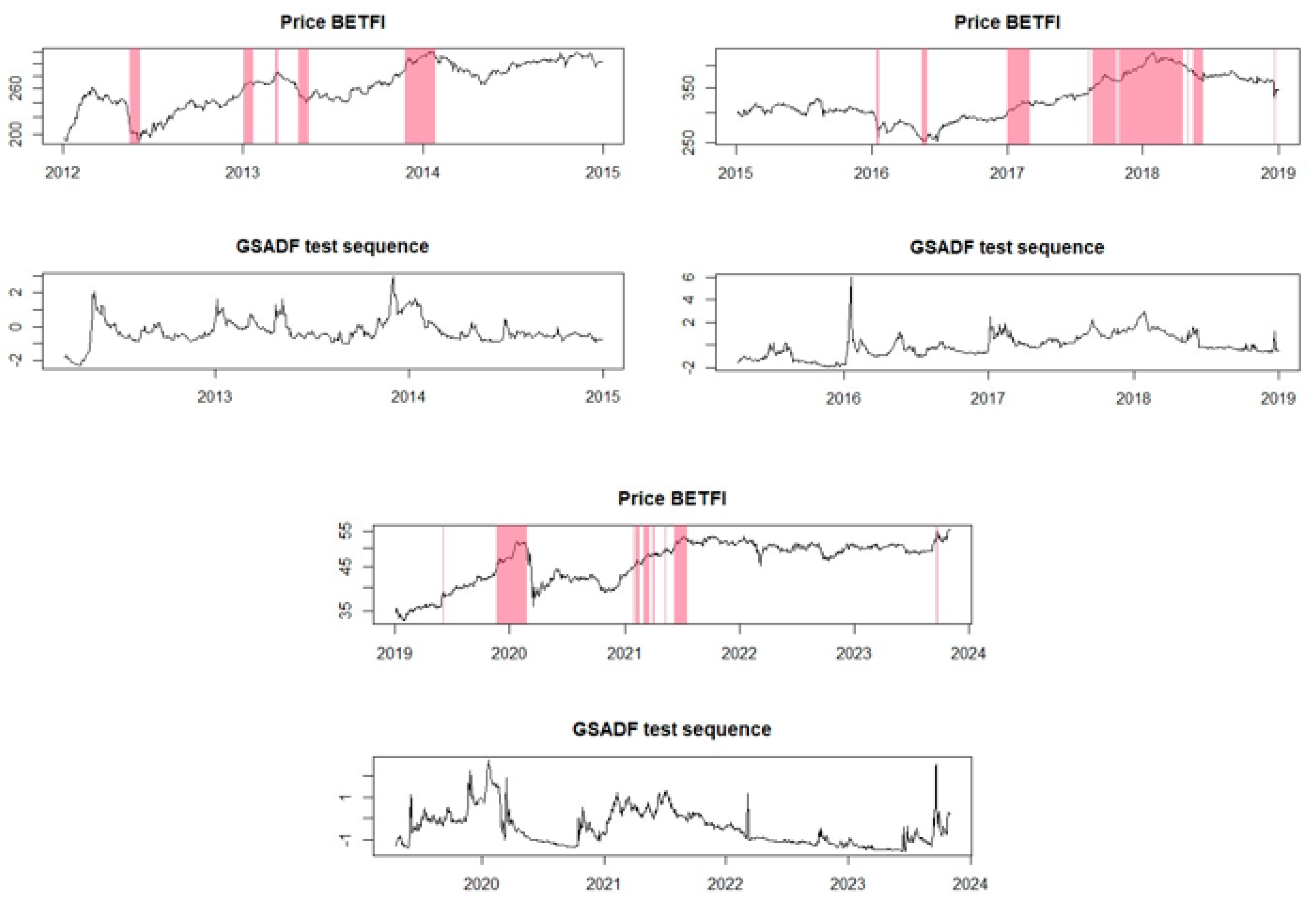
Regarding the financial bubble identification test using the GSADF method, it was conducted as shown in Figure 3. We can observe that there are periods similar to those identified as price bubbles using the EXCF method, but it also brings to light additional periods. For instance, the GSADF model highlighted potential price bubbles during the period 2012–2018, which the EXCF model did not identify. Thus, during this period, 10 time intervals were identified where these financial bubbles occurred. Additionally, the GSADF test confirmed the bubbles from the recent years analyzed, 2019–2023, also identified by the EXCF model.

To understand how these price bubbles of the BET-FI Index formed, we sought various information to identify possible factors underlying the formation of financial bubbles.

At the end of 2009, according to Finance Newspaper (2009), the BET-FI Index, which monitors the performance of five financial investment companies on the Bucharest Stock Exchange, recorded a 6% decline in Wednesday’s session, marking the most significant downturn in the last four months, amid a 4% overall market decline. The BET Index, representing the top ten most liquid companies, depreciated by 3.29%. This development followed a recorded major decline, influenced by the negative trend in European markets.

According to information from Banking News in 2015, the Bucharest Stock Exchange experienced a significant decline, and analysts believed that, in the absence of a rapid recovery in the Chinese economy, a more severe crisis than the one in 2008 could follow. On 24 August 2015, all stock exchanges faced a price shock, driven by the crisis in the Chinese economy, according to specialists’ opinions. This day was dubbed “Black Monday.” Stock exchanges in several Asian countries opened lower due to the dramatic fall of the Shanghai Stock Exchange. Financial market panic began with the depreciation of the yuan, the Chinese national currency. Economists argued that everything was triggered by the decision of major investment funds to withdraw their capital under investor pressures. The Shanghai Stock Exchange closed down 8.5%, the most drastic decline in the last eight years, initiating a domino effect, meaning a financial contagion.

According to the Bucharest Stock Exchange (2023) for the BET-FI Index, 2019 was the year the index registered one of its best rentabilities since its apparition (1995), considering that all of the market indexes had also registered exponential rentability growth (up to 47%, if we consider the BET-TR Index). This immense increase in the rentability of the index was mainly a result of Hidroelectrica being listed in the market, considering its very high importance in the Romanian market. Between late 2020 and late 2021, it seems like the BET-FI Index registered a significant increase due to the fact that the dividends have paid off for investors, showing a 40% return on investment.

It seems like the armed war between Russia and Ukraine triggered a decrease in the financial markets. Russia’s late February invasion of Ukraine caused a global shock within the financial markets, BET-FI included, right in the next month. Yet, until 2022, the BET-FI Index managed to partially recover from this event, mainly due to how the other financial markets evolved, but also due to the dividend’s proposal. Even though the index registered small ups and downs throughout 2021, the beginning of 2022 registered a decrease in the index caused by a “solidarity tax” imposed by the local government, a tax that reduced the index by 3.7% (Bursa.ro 2022).

As for the abovementioned period, Hidroelectrica played a crucial role in how Romania’s financial market evolved during this year. The main reason for the increase that we can observe at the end of the year is the 170,000 investors in the Hidroelectrica company that directly impacted the direction of the local financial markets, the BET-FI included (Forbes.ro 2023).

This analysis indicates that the evolution of the BET-FI Index has been influenced by several key factors, leading to distinct periods of financial bubble formation. For example, in 2019, a significant growth period of the index was observed, marking a potential positive bubble. This was largely attributed to the listing of Hidroelectrica, which held significant importance in the Romanian financial market. Investors benefited from substantial dividends, contributing to the index’s rise. Between the end of 2020 and the end of 2021, the BET-FI Index experienced significant growth, primarily due to dividend payments to investors, yielding a 40% return. This contributed to the formation of a potential positive bubble. Furthermore, the beginning of 2022 was marked by a decline in the index following Russia’s invasion of Ukraine. This geopolitical instability triggered a global shock in financial markets, impacting the BET-FI as well. However, the index managed a partial recovery, reflecting the evolution of other financial markets. Additionally, in 2023, Hidroelectrica continued to play a crucial role in the financial market’s evolution, significantly influencing the BET-FI Index.

In summary, the multiple financial bubbles identified in the analyzed period can be attributed to a complex mix of events, listings of significant companies, geopolitical factors, and government decisions. Each period of growth or decline reflects the specific dynamics of the Romanian financial market and the factors that influenced it during those moments. Furthermore, each period of growth or decline in the BET-FI Index can be understood in the context of financial contagion, where external events and internal decisions have an amplified impact on financial markets, directly influencing the index’s evolution. Financial contagion manifests through the rapid transmission of shocks and instability from one area of financial markets to others.

In Figure 4, the EXCF test was conducted to highlight financial bubbles for the S&P 500 index. In this case, the model identified six periods in which price bubbles formed, spanning from 2015 to 2023.

In 2015, the S&P 500 index experienced varied performance throughout the year. Concerns arose about the global economic growth slowdown, particularly in China (CNBC.com 2015). Weak economic data and volatility in global financial markets raised worries about their impact on American companies and the potential for a recession. Additionally, oil prices significantly declined in 2015, impacting energy sector companies and causing concerns about the overall health of the global economy. This had a negative effect on the stocks of many S&P 500 companies, as a significant number of them are either directly related to or have ties with the energy sector (Yahoo Finance 2016; The Guardian.com 2015).

In 2016 and 2017, the S&P 500 index exhibited positive performance, with relatively limited periods of decline during those years. In the first part of 2016, concerns about the health of the Chinese economy and financial market volatility negatively impacted the S&P 500. However, the market later rebounded, partly due to global economic stimuli. The presidential elections in November 2016 were a significant moment for financial markets. Following the election of the president, the initial market reaction was negative, but a reversal occurred, and the market showed positive trends, fueled by optimism regarding pro-business policies announced by the presidential administration (CNBC.com 2017a).

The year 2017 witnessed a strong rally in financial markets, including the S&P 500, amid expectations of tax cuts, deregulation, and fiscal incentives under the presidential administration. In 2017, the U.S. economy continued to grow, and companies reported robust profits. These factors supported the positive performance of the S&P 500 (CNBC.com 2017b).

Trade tensions between the United States and China escalated in 2018, with the mutual imposition of customs tariffs. Investors were concerned about the potential impacts of these tensions on global economic growth and corporate profitability (International Monetary Fund 2019).

The GSADF model sequence in Figure 5 also illustrates periods during which price bubbles were identified, similar to the EXCF model, starting from the year 2015 but extending until the year 2021. Therefore, we can conclude that the financial bubbles identified for the S&P500 index between 2015 and 2023 were influenced by various factors such as global economic concerns, presidential elections, and economic and trade tensions. All of these events can create panic among investors, leading to immediate decisions that may cause disruptions in the financial market.

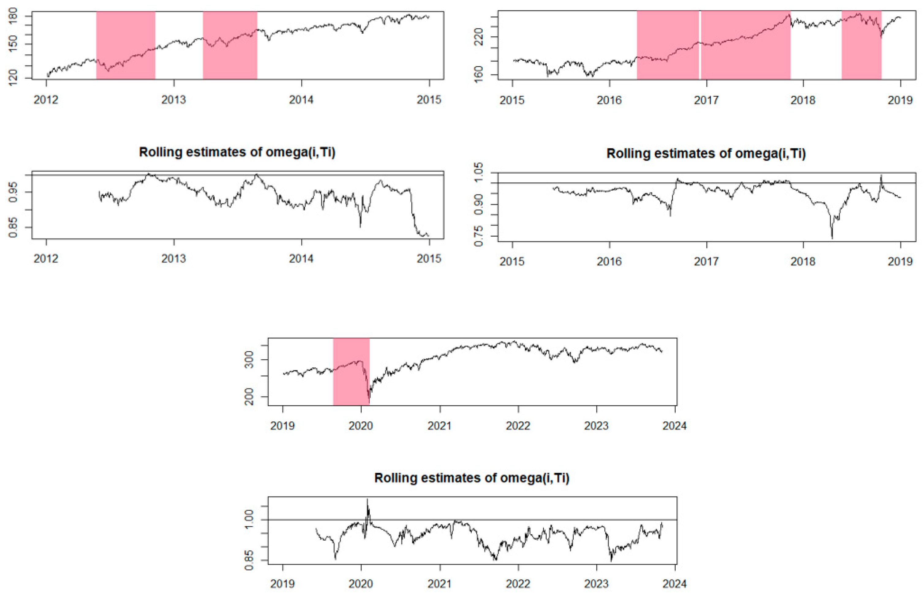
Regarding the IXIC index, the EXCF model was applied in Figure 6. It can be observed that the periods of identified financial bubbles are similar to those identified in the S&P 500 index.

In the first half of 2014, the IXIC index experienced robust growth, marked by significant increases and reaching new highs. The technology sector played a pivotal role in driving this growth, with companies such as Apple, Google, and Facebook delivering strong performances, contributing significantly to the index’s advancement. Additionally, the biotechnology sector saw significant growth during the same period, further adding to the rise of the IXIC. Smaller biotechnology companies recorded notable gains due to progress in drug development and positive results from clinical studies. All of these factors contributed to the formation of price bubbles (Techcrunch.com 2014).

Moreover, the other identified bubbles are justified by the same factors as those for the S&P 500, such as electoral elections, global concerns about economic growth, especially in China, but also factors like the performance growth of the tech sector (International Banker.com 2017). Additionally, the biotechnology and healthcare sectors were active contributors to the index’s volatility. The performance of smaller biotech firms and healthcare companies continued to impact the Nasdaq Composite’s movements.

Furthermore, the explosive growth of cryptocurrencies, especially Bitcoin, has captured the attention and interest of investors. While not directly linked to the IXIC index, this trend reflects an appetite for innovative assets with high growth potential among investors.

The GSADF test for the IXIC index can be identified in Figure 7. Unlike the EXCF model, this test identified fewer price bubbles for the analyzed index.

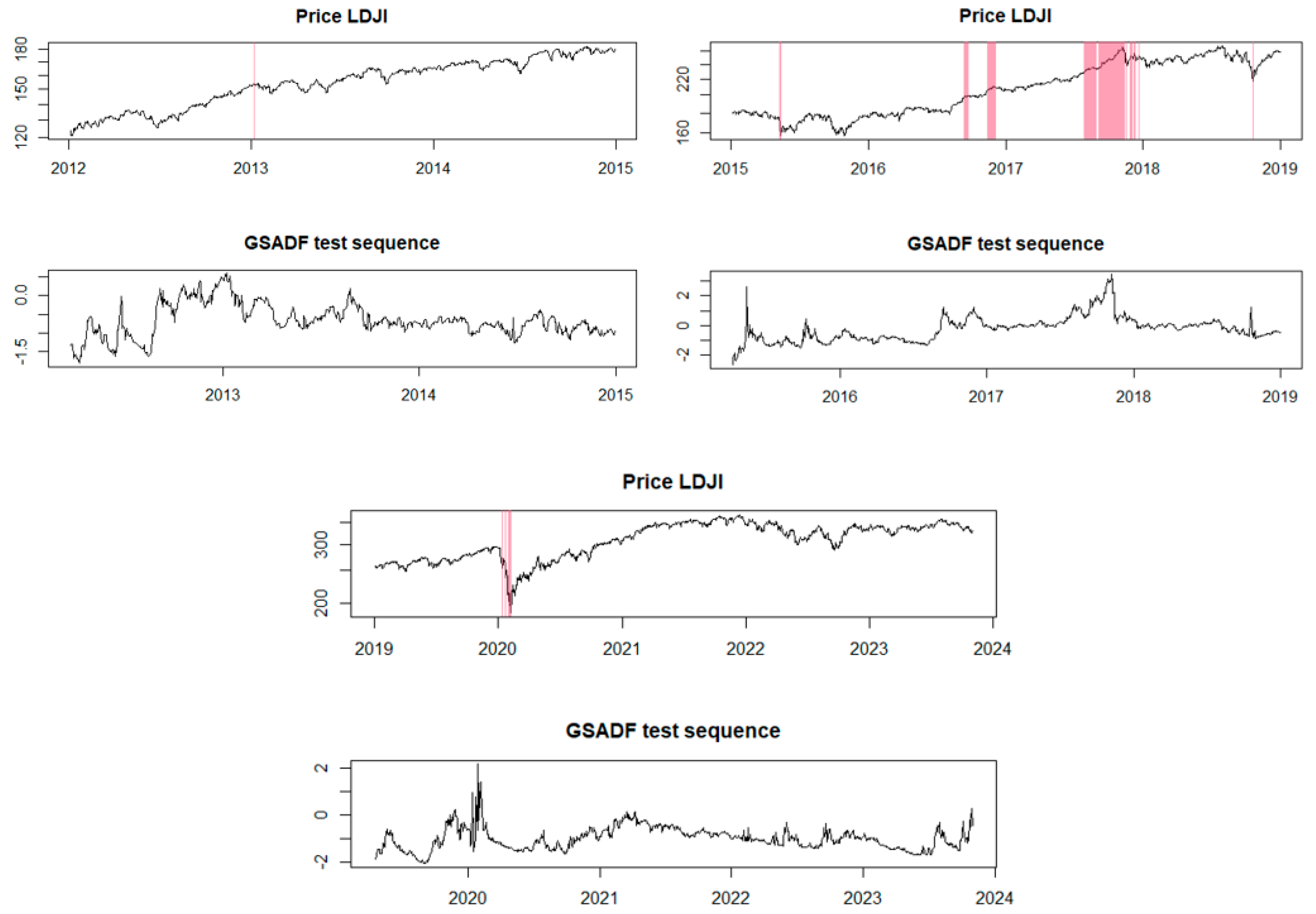
The EXCF model has been tested for the last index analyzed by us, the DJIA index. We observe in Figure 8 that six periods with financial bubbles have been identified. Both positive and negative bubbles are observed.

Additionally, the GSADF test also identified periods in which there were potential price bubbles for the DJIA index. In Figure 9, one can observe the periods marked for these price bubbles, which are relatively similar to the EXCF test but over shorter time frames.

All of these analyses highlight that political tensions, armed conflicts, and economic imbalances in major countries with systemic importance in the global economy, such as China, can generate contagion effects that affect the financial market. Investor panic and changes in investment behavior are also impacted and can contribute to the formation of price bubbles. Additionally, we observed for all of the analyzed indices that during the COVID-19 pandemic period, price bubbles were identified, emphasizing that the pandemic itself represented a factor in the formation of these bubbles.

The analysis in this section concludes with the determination of the Value at Risk (VaR) and Expected Shortfall (ES). The VaR is a measure of the maximum expected loss at a certain confidence level, expressed in percentages. The ES (Expected Shortfall) represents the expected value of losses in case they exceed the specified VaR level. These values can provide investors with useful information about the level of risk associated with the analyzed stock indices.

The graphs in Figure 10 depict the VaR (Value at Risk) and ES (Expected Shortfall) levels for the analyzed indices: BET-FI, S&P 500, IXIC, and DJIA. The blue horizontal line represents the 5% VaR level, while the green horizontal line indicates the 5% ES level. The VaR represents the maximum expected loss in the worst 5% of scenarios, while the ES represents the expected value of losses in the worst 5% of scenarios. The graphs track moments when the returns of the four analyzed indices exceed the estimated risk levels. It is observed that most of the instances where the risk level was exceeded coincide with periods when the analyzed stock indices were in a negative or positive bubble. This may suggest that, despite the financial market being quite volatile, it is not advisable to invest during periods of identified financial bubbles.

4.2. Exploring Stock Index Modeling with ARDL: Insights into Performance Metrics

This study delved into the complex world of financial indices, with a specific focus on the BET-FI as the dependent variable. Through advanced econometric techniques, we aimed to uncover hidden patterns, assess the impact of various factors, and provide valuable predictive insights into the performance of stock indices. According to Nica et al. (2023a), the ARDL model stands out as a flexible instrument for scrutinizing time series data and unraveling relationships among research variables. Its proficiency in addressing both short-term and long-term dynamics, as well as handling cointegration and ensuring robustness, renders it indispensable for empirical research. This section delves into the fundamental steps of applying the ARDL model to our dataset. Descriptive statistics play a crucial role in comprehending and priming the data before implementing the ARDL model.

Table 2. Summary statistics.

Statistics	BET-FI	S&P 500	IXIC	DJIA
Mean	10.45	7.81	8.76	9.97
Median	10.41	7.80	8.74	9.98
Maximum	10.87	8.46	9.65	10.50
Minimum	9.90	7.17	7.94	9.42
Std. Dev.	0.25	0.34	0.48	0.30
Skewness	0.05	0.09	0.14	0.01
Kurtosis	1.98	2.11	1.98	1.81
Jarque–Bera	5.69	4.50	6.15	7.72
Probability	0.08	0.10	0.07	0.06

provides a detailed overview of the basic statistical characteristics of the data distribution for the BET-FI, S&P 500, IXIC, and DJIA indices. Statistics such as mean, median, minimum and maximum values, standard deviation, skewness, kurtosis, and the Jarque–Bera test for normality of skewness and kurtosis are presented. According to the information in Table 2, all indices have median values close to the means, suggesting a relatively symmetric distribution around the central value. Additionally, small standard deviations indicate a relatively tight concentration of values around the mean. Skewness values close to zero indicate a relatively symmetric distribution for the analyzed stock indices, and the kurtosis values suggest that the peaks of the distributions are generally within the normal range, reflecting a moderate concentration around the mean. For all indices, the Jarque–Bera values are significant at a significance level of 0.10 or 0.08, suggesting a small deviation from a normal distribution.

In

Table 3. (a) ADF Unit Root Test (intercept). (b) ADF Unit Root Test (trend and intercept).

(a)
Variables	Level	First Difference	Order of Integration
	t-Statistics	t-Statistics
BET-FI	−1.28 (0.63)	−10.95 (0.00)	I(1)
S&P 500	−1.32 (0.61)	−13.28 (0.00)	I(1)
IXIC	−1.39 (0.58)	−12.40 (0.00)	I(1)
DJIA	−1.09 (0.71)	−12.92 (0.00)	I(1)
(b)
Variables	Level	First Difference	Order of Integration
	t-Statistics	t-Statistics
BET-FI	−3.39 (0.05)	−10.90 (0.00)	I(1)
S&P 500	−3.12 (0.10)	−13.27 (0.00)	I(1)
IXIC	−1.72 (0.73)	−12.41 (0.00)	I(1)
DJIA	−3.66 (0.02)	−12.88 (0.00)	I(1)

, the results of the Augmented Dickey–Fuller test are presented, indicating whether the time series of the analyzed variables has a unit root and providing information about the order of integration required to make these series stationary. At that level, the t-statistics coefficient is −1.28, with a probability (p-value) of 0.63. However, upon applying the first differencing, the t-statistics coefficient becomes significant at −10.95, with a probability of 0.00. This result suggests that the BET-FI variable requires differencing to become stationary, and the order of integration is I(1). Similarly, for the S&P 500, at that level, we have a t-statistics coefficient of −1.32 with a probability of 0.61, and through differencing the data once, the coefficient becomes significant at −13.28, with a probability of 0.00. This also indicates an order of integration of I(1). The same observations hold for the variables IXIC and DJIA. At that level, the t-statistics coefficients are not significant, but they become significant upon differencing the data once, and the order of integration is I(1). In the case of the ADF test, which includes both the intercept and trend, the results are similar. The t-statistics coefficients become significant at that level (with the intercept) and become even more significant upon differencing once. The order of integration for all variables is I(1). According to (Shrestha and Bhatta 2018), an Autoregressive Distributed Lag (ARDL) model represents a regression model based on Ordinary Least Squares (OLS) methodology. It is suitable for analyzing both non-stationary time series and time series with a mixed order of integration. The ARDL model incorporates an adequate number of lags to effectively capture the underlying data-generating process within a general-to-specific modeling framework.

The subsequent step involves determining the suitable lag structure for the ARDL model, as outlined in Figure A1 from Appendix A.

Enders (2014) emphasized the importance of meticulously choosing the optimal lag length before implementing the ARDL model. This step is critical for several reasons, including ensuring the model’s proper alignment with the data. A lag length that is too short could lead to the model missing key dynamics, potentially causing an omitted variable bias.

Table 4. The outcomes of the cointegration bounds test.

Test Statistic	Value	K (Number of Regressors)
F-statistic	6.61	3
Critical value bounds (Finite sample n = 80)
Significance	I(0)	I(1)
10%	2.47	3.31
5%	2.92	3.83
1%	3.90	5.04

displays the outcomes of the cointegration bounds test, designed to explore the existence of long-term causality. The F-statistic, computed at 6.61, exceeds the critical upper bounds associated with I(1), signifying the presence of cointegration among the variables under scrutiny. In this instance, the chosen model is ARDL (1, 0, 2, 0).

The results of the cointegration bounds test (ARDL) indicate that the F-statistic is relevant for analyzing the cointegration among the involved variables. The F-statistic values, along with critical bounds for different significance levels, are presented in Table 4. Since the F-statistic exceeds all critical values for a significance level of 1%, there is cointegration among the analyzed variables at a confidence level of 99%. This suggests a stable, long-term relationship between the respective variables.

The use of the Error Correction Model (ECM) equation is crucial for understanding short-term adjustments toward long-term equilibrium. In

Table 5. The long-run estimated coefficients (restricted constant and no trend).

Variables	Coefficient	t-Statistics	Prob.
S&P 500	1.31	2.04	0.04
IXIC	−0.75	−2.06	0.04
DJIA	0.55	1.42	0.15
C	1.20	0.80	0.12

, it is observed that for each unit increase in the S&P 500, a corresponding increase of 1.31 units in the dependent variable BET-FI is expected in the long term. This result is significant at a 0.05 significance level. Regarding the IXIC index, for each unit increase, a corresponding decrease of 0.75 units in the dependent variable BET-FI is anticipated in the long term. This result is significant at a 0.05 significance level. The constant term, denoted as C, represents the expected value of the dependent variable BET-FI in the long term when all other regressors are zero. Although it is not significant at a 0.05 significance level, it contributes to the baseline level of the dependent variable. Also, in Equation (10), the mathematical form of the error correction term has been represented, indicating the short-term adjustments of the variable BET-FI toward the long-term equilibrium determined by the regressors included in the model.

$$EC=BETFI-(1.31\times SP500-0.75\times IXIC+0.55\times DJIA+1.20)$$

(10)

In

Table 6. The short-run ARDL estimation.

Variables	Coefficient	t-Statistics	Prob.
D(IXIC)	0.16	2.11	0.03
D(IXIC (−1))	0.22	3.37	0.00
CointEq (−1) *	−0.22	−5.84	0.00
R-squared			0.39
Adjusted R-squared			0.39
Log likelihood			246.14
Durbin–Watson stat			1.82
Akaike info criterion			−3.75
Schwarz criterion			−3.67
Hannan–Quinn criterion			−3.71

, the ARDL Error Correction Regression was employed to estimate short-term adjustments within the ARDL model. This type of regression is crucial for assessing the immediate impact of temporary deviations from long-term equilibrium, as well as for studying the dynamics of variables within the model. Thus, we observe that for a one-unit increase in the D(IXIC) (the first difference of the IXIC), a corresponding short-term increase of 0.16 units is expected in the dependent variable BET-FI. This result is significant at a 0.05 significance level. Additionally, a 0.22-unit increase in D(IXIC) in the previous period (a lagged difference of the IXIC) is associated with a significant short-term increase of 0.22 units in the dependent variable BET-FI. This result is significant at a 0.01 significance level. The symbol “*” signifies that this variable is lagged by one period in the regression model. The error correction term indicates adjustments toward long-term equilibrium. A negative coefficient suggests a negative correction toward equilibrium in the short term. This term is significant and contributes to immediate adjustments of the variables. Regarding the model quality metrics, the coefficient of determination (R-squared) indicates the proportion of variance in the dependent variable explained by the model. Measures of the AIC, BIC, and HQC criteria are used to evaluate the model efficiency, with lower values indicating a better model. The Durbin–Watson statistic measures the autocorrelation of residuals, with a value close to two indicating the absence of autocorrelation.

Regarding the diagnosis of coefficients, a coefficient confidence interval test was conducted. The confidence interval (CI) for the variables analyzed in our ARDL model indicates the range in which the respective coefficients are likely to fall with a certain level of confidence. For example, as shown in

Table A2. Coefficient confidence intervals.

		90% CI		95% CI		99% CI
Variables	Coefficient	Low	High	Low	High	Low	High
BET-FI (-1)	0.77	0.69	0.85	0.68	0.87	0.65	0.90
S&P 500	0.29	0.07	0.50	0.03	0.55	−0.05	0.63
IXIC	0.16	0.01	0.32	−0.01	0.34	−0.07	0.40
IXIC (-1)	−0.11	−0.27	0.04	−0.30	0.07	−0.36	0.13
IXIC (-2)	−0.22	−0.33	−0.10	−0.36	−0.08	−0.40	−0.03
DJIA	0.12	−0.02	0.26	−0.05	0.29	−0.10	−0.35
C	0.26	−0.33	0.86	−0.45	0.98	−0.68	1.21

from Appendix A, the estimated coefficient for the BET-FI (−1) is 0.77, and the 99% confidence interval is [0.65, 0.90]. This interval indicates with 99% confidence that the true coefficient of the BET-FI (−1) variable is between 0.65 and 0.90. The values for the all confidence intervals are presented in Table A2 from Appendix A.

To conduct the residuals diagnosis, a histogram–normality test was performed. Figure 11 presents information about the distribution of the residuals. The value of the mean very close to zero indicates that the mean of the residuals is close to zero, which is positive for the accuracy of the model. Similar to the mean, a median close to zero suggests symmetry in the distribution of the residuals. The maximum and minimum values indicate the range in which the residuals fall. The fact that these values are relatively small may suggest a good fit of the model. The low standard deviation value of 0.03 indicates a low dispersion of the residuals around the mean, suggesting a better fit of the model. The Jarque–Bera test checks whether the residuals have a normal distribution. A lower probability suggests a significant deviation from normality. In our model, the probability is 0.09, suggesting that there is not enough evidence to reject the null hypothesis of normality at a significance level of 0.05.

To check for signs of functional misspecification in the model, the Ramsey reset test was employed, and the results are presented in

Table 7. (a) Ramsey reset test. (b) Unrestricted test equation.

(a)
Test	Value	df	Probability
t-statistic	1.04	122	0.29
F-statistic	1.08	(1, 122)	0.29
Likelihood ratio	1.15	1	0.28
F-test summary
Test	Sum of Sq.	df	Mean Squares
Test SSR	0.00	1	0.00
Restricted SSR	0.17	123	0.00
Unrestricted SSR	0.17	122	0.00
LR test summary
Test	Value
Restricted LogL	246.14
Unrestricted LogL	246.72
(b)
Variable	Coefficient	t-Statistic	Probability
BET-FI(-1)	−0.16	−0.18	0.85
S&P 500	−0.07	−0.20	0.83
IXIC	−0.03	−0.15	0.87
IXIC (-1)	0.02	0.15	0.87
IXIC (-2)	0.04	0.15	0.87
DJIA	−0.01	−0.06	0.94
C	6.24	1.08	0.27
FITTED^2	0.05	1.04	0.29
R-squared	0.97
Log likelihood	246.72
F-statistic	797.81
Prob (F-statistic)	0.00

. For the restricted model (original), the probabilities associated with the t-statistics, F-statistic, and likelihood ratio are quite high (0.29 and 0.28). This suggests that there is not enough evidence to reject the null hypothesis of correct model specification. Therefore, the original model seems to be well-specified. Regarding the unrestricted model, probabilities around 0.85 indicate that there is not enough evidence to reject the null hypothesis of correct specification for the unrestricted model either. The high R-squared (97%) indicates a good fit of the data within the unrestricted model.

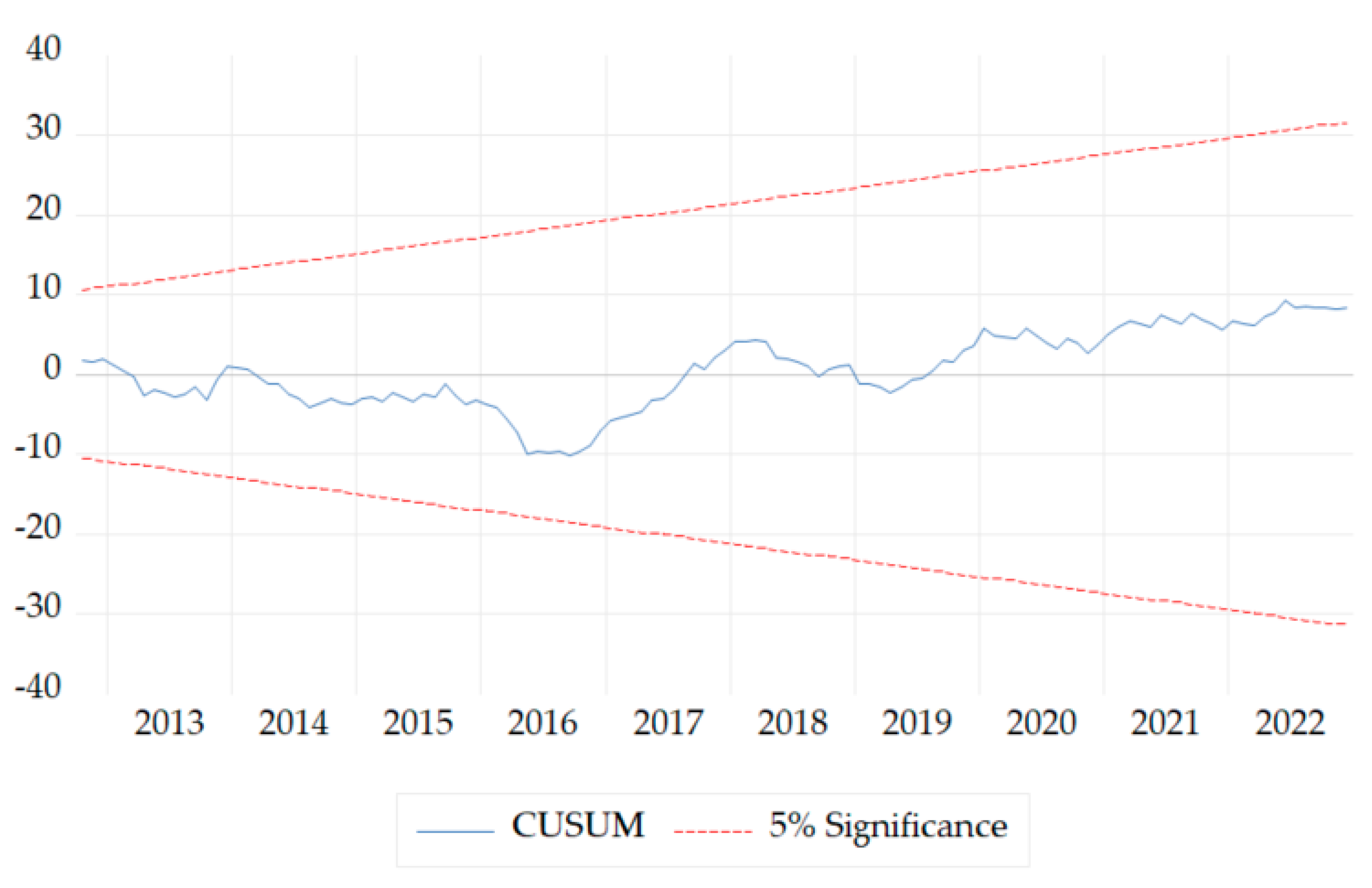
The CUSUM test is a method used to assess the stability of a model over time. In Figure 12, we can observe the blue line (CUSUM) constructed to track the cumulative sums of residuals from the model as we observe new data. There are two critical significance lines (red) at 5%. Given that the CUSUM line does not cross the significance critical lines, this suggests that the model is stable, and there are no significant signs of performance degradation over time.

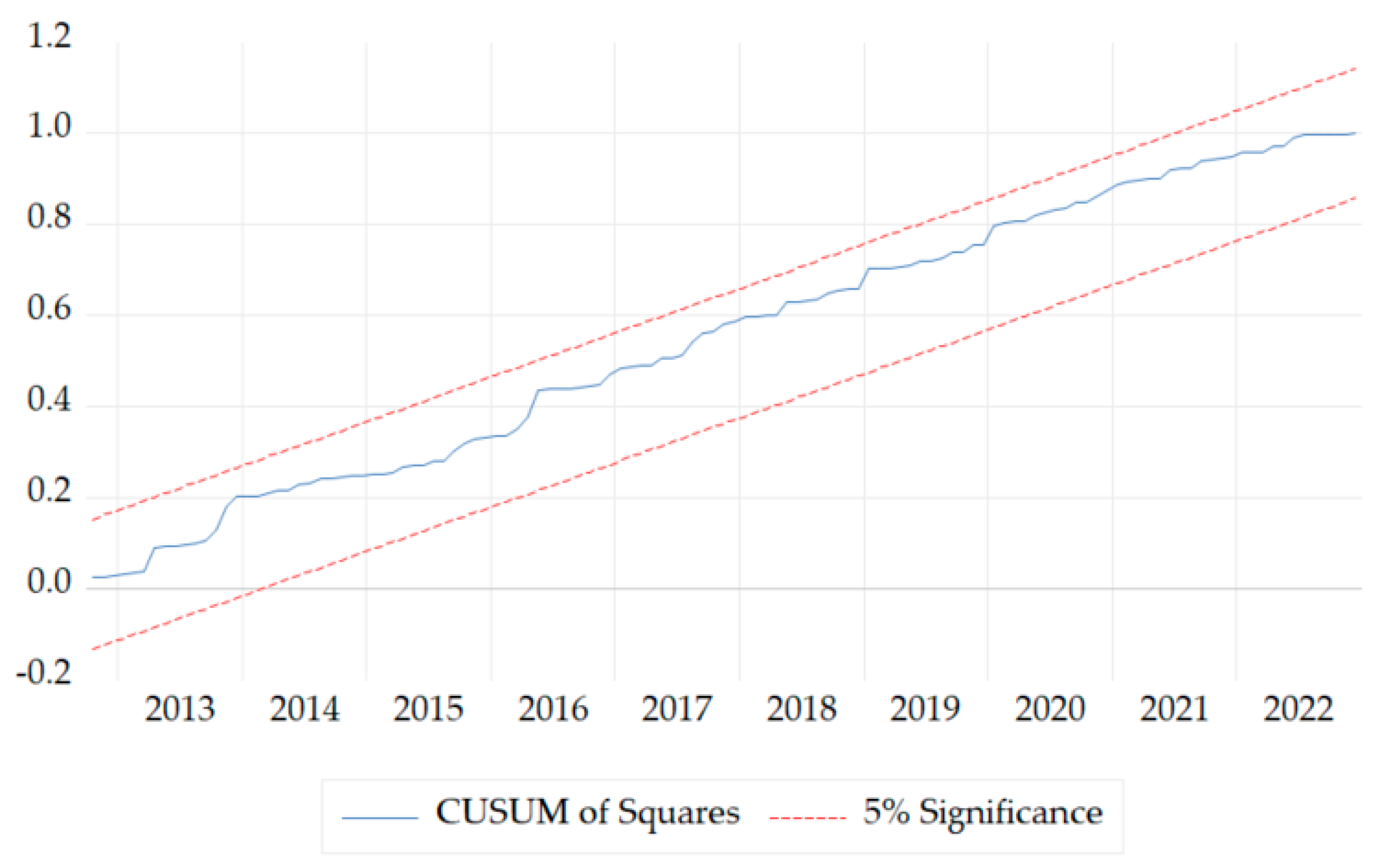
Regarding the graph in Figure 13, CUSUM of squares refers to a CUSUM plot based on the squares of the residuals or the squares of the differences between the observed values and those predicted by the model. This CUSUM plot is used to assess the model’s stability over time concerning the variability of the residuals. If the CUSUM of squares line moves consistently and does not cross the critical significance lines, it indicates stability in the variability of the residuals. Overall, a CUSUM of squares plot provides information about significant changes in residual variability and can help identify moments when the model might require adjustments.

In order to provide a more comprehensive analysis and strengthen the obtained results, the VAR model results from

Table A3. Vector autoregression estimates.

Variables	BET-FI	SP500	IXIC	DJIA
BET-FI (-1)	0.82 (0.10)	−0.03 (0.09)	−0.00 (0.10)	−0.05 (0.09)
BET-FI (-2)	−0.07 (0.09)	−0.01 (0.08)	−0.02 (0.10)	0.00 (0.08)
S&P 500 (-1)	0.11 (0.68)	−0.03 (0.61)	−1.56 (0.71)	−0.73 (0.62)
S&P 500 (-2)	−0.01 (0.68)	0.69 (0.61)	1.13 (0.72)	0.48 (0.62)
IXIC (-1)	0.05 (0.31)	0.30 (0.28)	1.56 (0.33)	1.91 (0.29)
IXIC (-2)	−0.07 (0.32)	−0.06 (0.29)	−0.31 (0.34)	0.02 (0.29)
DJIA (-1)	0.14 (0.42)	0.47 (0.29)	0.70 (0.44)	1.33 (0.38)
DJIA (-2)	−0.01 (0.42)	−0.45 (0.37)	−0.62 (0.45)	−0.35 (0.39)
C	0.82 (0.44)	0.83 (0.39)	0.67 (0.46)	0.93 (0.40)
R-squared	0.96	0.98	0.99	0.98
Adjusted R-squared	0.96	0.98	0.99	0.98
S.E. equation	0.04	0.04	0.04	0.04
Akaike AIC	−3.30	−3.51	−3.19	−3.47
Schwartz SC	−3.10	−3.31	−2.99	−3.27

in Appendix A provides estimates of the lagged effects of variability in stock indices and measures for assessing the model’s quality. According to the values of R-squared and adjusted R-squared, we can confirm that the observed data fit the model. Additionally, the standard error equation shows that the results are precise, considering the very low values. In Figure 14, the variance decomposition using Cholesky factors for different periods and the analyzed stock indices have been illustrated. Numeric values are presented in

Table A1. Variance decomposition using Cholesky factors.

Variables	Period	BET-FI	S&P 500	IXIC	DJIA
BET-FI	1	100.00	0.00	0.00	0.00
	5	88.77	10.34	0.02	0.86
	10	76.09	19.97	1.28	2.64
	15	65.87	22.60	6.93	4.59
	20	57.10	21.58	14.50	6.80
S&P 500	1	29.12	70.87	0.00	0.00
	5	24.46	69.58	4.59	1.35
	10	19.79	55.79	21.92	2.49
	15	16.92	41.85	36.97	4.29
	20	15.30	32.55	45.22	6.91
IXIC	1	28.05	60.48	11.46	0.00
	5	22.16	44.82	30.72	2.27
	10	17.50	31.58	46.56	4.34
	15	15.26	23.44	54.19	7.09
	20	14.09	18.70	56.64	10.55
DJIA	1	28.30	63.02	3.27	5.39
	5	21.21	64.40	2.29	12.08
	10	17.94	58.52	8.45	15.07
	15	15.91	47.57	19.31	17.20
	20	14.58	38.40	27.42	19.58

in Appendix A, representing the percentages of the total variation in each stock index explained by Cholesky factors in different periods. For instance, as observed in Figure 15, for the BET-FI Index in period 1, the entire variation (100%) is explained by the Cholesky factor associated with the BET-FI. In subsequent periods (5, 10, 15, and 20), a gradual reduction in the relative contribution of the Cholesky factor associated with the BET-FI to the total variance is noticeable. Similar to the BET-FI, each stock index has its own associated Cholesky factor. Overall, Cholesky factors associated with the respective stock indices have a significant contribution in period 1. As time progresses, the relative contribution of these factors decreases, suggesting that other factors (other stock indices and additional factors) begin to play a more prominent role in explaining the variation. In subsequent periods, a redistribution of variance among the stock indices is observed, indicating changes in the interactions and their impact on variation. From the perspective of financial contagion effects, Cholesky factors indicate how the variability of one stock index is correlated with others. A strong correlation may suggest that changes in one index are associated with similar or opposite changes in other indices, thereby indicating interdependence.

Historical decomposition using generalized weights is a method employed in time series analysis that decomposes the historical movements of a variable of interest into the contributions of various shocks or structural innovations that occurred in the past (Figure 15). The interpretation of the historical decomposition graph is achieved by analyzing the individual contributions of the factors to the total variation of the variable. Each line or component of the graph represents the relative contribution of a specific factor or shock to the movements of the variable at a particular point in time. For example, the first graph illustrating the decomposition of the BET-FI includes different time series such as “actuals,” “baseline,” “baseline+BET-FI,” “baseline+S&P 500,” “baseline+IXIC,” and “baseline+DJIA.” “Actuals” represents the time series of the BET-FI variable in this case. “Baseline” depicts the evolution of the BET-FI Index in the absence of other factors or additional influences, serving as a baseline for comparison and showing how the variable would evolve if there were no external factors. The other lines represent how the BET-FI evolves, influenced only by the S&P 500 factor (green line), only by the IXIC factor (red line), or only by the DJIA factor (black line). We observed differences between the actuals and baseline, indicating the impact of the other indices or external influences on the actual time series.

According to the results in

Table 8. (a) ARDL model. (b) Performance metrics of the ARDL model.

(a)
Variables	Coefficient	Std. Error	t-Statistics	Prob.
BET-FI(−1)	0.77	0.04	16.03	0.00
S&P 500	0.29	0.13	2.22	0.02
IXIC	0.16	0.09	1.84	0.06
IXIC(−1)	−0.11	0.09	−1.21	0.22
IXIC(−2)	−0.22	0.07	−3.15	0.00
DJIA	0.12	0.08	1.40	0.16
C	0.26	0.36	0.73	0.46
(b)
R-squared	0.97	Mean dependent var		10.45
Adjusted R-squared	0.97	S.D. dependent var		0.24
S.E. of regression	0.03	Akaike info criterion		−3.67
Sum squared resid	0.17	Schwarz criterion		−3.52
Log likelihood	246.14	Hannan–Quinn criterion		−3.61
F-statistic	929.93	Durbin–Watson stat		1.82
Prob (F-statistic)	0.00

, the mathematical form of the ARDL (1, 0, 2, 0) model has been written in Equation (11), where the dependent variable is the BET-FI Index, and the independent variables are the S&P 500, IXIC, and DJIA indices. The specification (1, 0, 2, 0) of the ARDL model means that it uses an autoregressive order of 1, indicating that a previous period of the dependent variable is included; an integration order of 0, meaning that the variables have not been differenced to become stationary; a moving average order of 2, indicating that two moving average terms are included in the model (IXIC(-1) and IXIC(-2)); and the last parameter in the specification, 0, refers to the fact that no seasonal components are included. In the case of BET-FI (-1), the coefficient of 0.77 indicates that an increase by one unit in the BET-FI variable in the previous period is associated with an increase of 0.77 units in the BET-FI variable in the current period. The coefficient for the S&P 500 index is 0.29, suggesting that an increase by one unit in the S&P 500 variable is associated with an increase of 0.29 units in the BET-FI variable. Regarding the IXIC index, the coefficient is 0.16, indicating that an increase by one unit in the IXIC variable is associated with an increase of 0.16 units in the BET-FI variable. The coefficient is −0.11 for IXIC (-1), suggesting that an increase by one unit in the lagged value of the IXIC variable is associated with a decrease of −0.11 units in the BET-FI variable. Also, the coefficient of 0.22 for IXIC (-2) indicates that an increase by one unit in the second lagged values of the IXIC variable is associated with a decrease of −0.22 units in the BET-FI variable. Regarding the DJIA index, an increase by one unit in the DJIA variable is associated with an increase of 0.12 units in the BET-FI variable. According to the results of the model, the equation can be written in accordance with Equation (11).

$$\begin{array}{cc}BETFI=0.77 \times \hfill & BETFI\left(-1\right)+0.29\times SP500+0.16\times IXIC-0.11\times IXIC\left(-1\right)-0.22\times IXIC\left(-2\right)\hfill \\ & +0.12\times DJIA+0.26\hfill \end{array}$$

(11)

From the perspective of the ARDL model’s performance, the R-squared value is 0.97, indicating that the model explains approximately 97% of the variation in the dependent variable. The F-statistic value indicates that the model is globally significant, and the Durbin–Watson test suggests that the residuals do not have significant autocorrelation. The low values of the AIC, Schwarz, and log-likelihood metrics indicate a good model, with these metrics used to evaluate the efficiency of the model. Regarding the prediction of the dependent variable, it has been illustrated in Figure 16.

To assess the forecast quality, metrics such as RMSE (root mean squared error), MAE (mean absolute error), MAPE (mean absolute percent error), bias proportion, covariance proportion, and Theil’s U2 coefficient were used. RMSE measures the dispersion between the predicted and observed values. The lower the RMSE value, the higher the model’s accuracy. MAE is the average of the absolute differences between the forecasts and observations. A lower value indicates higher accuracy. MAPE measures the percentage of absolute error relative to the observed values. Theil’s coefficient compares the variability of the forecasts to the variability of the observations. A lower value suggests a more precise forecast. Bias proportion indicates the percentage of average error (bias) relative to the mean of observations. A very low value indicates no tendency to over- or under-estimate forecasts. Covariance proportion indicates the percentage of covariance between the forecasts and observations relative to the variance of the observations. A high value, close to one, suggests good agreement between the forecasts and observations. Theil’s U2 coefficient provides a measure of forecast quality relative to a simple base forecast (e.g., the mean). A lower value indicates better accuracy, and a value of 1.29 suggests that our forecast is better than a simple base forecast.

5. Discussion, Conclusions, and Policy Recommendations

Our study comprehensively and in detail addresses the complex interactions and potential risk of financial contagion among major financial indices, with a specific focus on the financial market of Romania. This offers a new and in-depth perspective on the dynamics of financial markets, which is essential in today’s globally interconnected context. Additionally, covering an extended period (2012–2023) allows for a comprehensive evaluation of long-term trends and the impact of major events such as the COVID-19 pandemic or geopolitical tensions, with our results being consistent with other research that has analyzed how the pandemic has affected financial markets. The behavior of investors, such as panic or fear, is quickly evident when certain events occur, like the pandemic crisis. Zhang et al. (2020) support in their study the fact that financial markets have been strongly impacted by the pandemic context and have recommended political interventions to stabilize the capital markets.

The use of the EXCF and GSADF models is based on their superior ability to identify and analyze price bubbles in financial indices. Unlike the GARCH model, which is excellent for assessing volatility and has been widely used in analyzing the volatility of financial markets, EXCF and GSADF are specifically designed to detect bubbles and periods of asset overvaluation, possessing the capability to capture more subtle and complex market dynamics that can predict the formation of bubbles. The choice of these methods is based on a careful review of the current state of knowledge in which numerous studies (Phillips et al. 2015a; Phillips et al. 2015b; Li et al. 2020; Liaqat et al. 2019; Dinçer et al. 2021) have demonstrated the usefulness of these methods in detecting price bubbles.

The EXCF method for the BET-FI, IXIC, and S&P500 indices highlights a potential financial bubble in 2023, which could be justified by the panic created among investors due to the Russia–Ukraine armed conflict, as also supported by Yousaf et al. (2022) in their study that the armed conflict has strongly affected the financial market.

In the dynamic world of financial markets, detecting and understanding the complex phenomenon of price bubbles is a crucial challenge for investors, analysts, and decision-makers in the financial sector. In this context, the use of advanced models such as EXCF and GSADF becomes essential for evaluating and anticipating price movements within benchmark indices such as the BET-FI, DJIA, IXIC, and S&P 500. The significance of employing EXCF and GSADF in analyzing financial indices like the BET-FI, DJIA, IXIC, and S&P 500 becomes evident amid high volatility and rapid changes in global markets. The results of applying the EXCF and GSADF methods have highlighted that various geopolitical events, the COVID-19 pandemic, or sudden changes in the national and global economy can generate instability in the financial market, both in Romania and worldwide. Our findings are consistent with other current research, even though their authors used different methods to analyze financial bubbles. Identifying price bubbles in these indices is vital for investors and decision-makers, providing them with the opportunity to adjust their strategies and manage risks efficiently. On the other hand, the analysis of price bubble detection is complemented by using the ARDL model, where the BET-FI serves as the dependent variable, while the S&P 500, DJIA, and IXIC act as independent variables. The ARDL model was used to assess the relationships among variables, interdependencies, influences, causality, and financial contagion effects. The BET-FI, as the dependent variable, represents the BET-FI index, reflecting the overall performance of the financial market in Romania. Modeling this variable allows for understanding its impact and interactions with other relevant variables. Thus, the ARDL model can reveal whether and how changes in independent variables can influence the BET-FI, highlighting connections and interdependencies between financial markets. Additionally, the ARDL model provides the opportunity to analyze relationships in the short and long term, allowing the identification of immediate effects and adjustments in the dependent variable’s response to changes in independent variables. The results of the ARDL model can offer valuable insights for making strategic decisions, managing risks, and developing more effective strategies in financial markets.

As financial markets are interconnected, the phenomenon of financial contagion becomes a crucial component. Identifying a bubble in a major index, such as the S&P 500, can influence the behavior of other indices, such as the BET-FI, DJIA, and IXIC. By using EXCF and GSADF to examine these interdependencies, we have gained a broader and more precise view of how changes in one index can propagate and affect the entire financial landscape.

The EXCF model uses continuous estimates to provide information about volatility variation and significant changes in the dynamics of the analyzed time series. These estimates offer insight into how volatility changes over time and can help identify periods where it increases significantly, indicating potential points of interest for the analysis of financial bubbles. Interpreting these continuous estimates is performed in the context of the analyzed time series. When continuous estimates show higher values, this suggests increased volatility in those periods, which may be associated with significant potential changes in market prices. Overall, areas with high values of continuous estimates can draw attention to periods where there is an increased probability of a financial bubble formation or significant market events. Through this integrated analysis, we aimed to make a significant contribution to understanding the dynamics of financial markets, enabling investors and decision-makers to approach the risks associated with price bubbles with greater confidence and develop more informed strategies in the face of global market challenges.

ARDL Error Correction Regression was applied to analyze short-term adjustments within the ARDL model. The findings revealed that a one-unit increase in the first difference of the IXIC corresponds to a significant short-term increase of 0.16 units in the dependent variable BET-FI, at a 0.05 significance level. Moreover, a 0.22-unit increase in the lagged difference of the IXIC in the previous period is associated with a substantial short-term increase of 0.22 units in the BET-FI, significant at a 0.01 significance level. The error correction term indicates adjustments toward long-term equilibrium, with a negative coefficient signifying a negative correction in the short term. This term is significant and contributes to immediate adjustments of the variables.

The Error Correction Model equation plays a crucial role in understanding short-term adjustments toward long-term equilibrium. The analysis in Table 5 revealed that a one-unit increase in the S&P 500 is associated with a significant long-term increase of 1.31 units in the dependent variable BET-FI, with a 0.05 significance level. Conversely, for each unit increase in the IXIC index, a significant long-term decrease of 0.75 units in the BET-FI is anticipated at the 0.05 significance level. While the constant term is not statistically significant at the 0.05 level, it contributes to the baseline level of the BET-FI.

Additionally, the results of the cointegration bounds test demonstrated the relevance of the F-statistic for analyzing cointegration among the variables. The F-statistic exceeds critical values for a 1% significance level, indicating cointegration among the variables with a 99% confidence level. This implies a stable long-term relationship between the analyzed variables, providing valuable insights into their interconnected dynamics.

The application of historical decomposition using generalized weights in time series analysis provides a nuanced understanding of the historical movements of the BET-FI variable. A graphical representation allows for the dissection of these movements into contributions from various shocks or structural innovations. By examining different components such as “actuals,” “baseline,” and factors like the S&P 500, IXIC, and DJIA, we can discern the individual influences of each factor on the BET-FI over time. The method illuminates how the variable would evolve in isolation and highlights the impact of external influences, contributing to a comprehensive analysis of the historical dynamics of the BET-FI in the context of multiple contributing factors.

The results of the analysis using the ARDL (1, 0, 2, 0) model revealed complex relationships between the BET-FI and the other variables, namely the S&P 500, IXIC, and DJIA. The obtained coefficients provide insights into the impact and direction of changes in these variables on the BET-FI. Notably, the positive coefficient for BET-FI (−1) indicates a positive correlation between the previous values of the BET-FI and the current ones. For the S&P 500, a positive coefficient suggests a positive association between its increase and positive evolution of the BET-FI. In the case of the IXIC, a positive coefficient for the IXIC and negative coefficients for IXIC (−1) and IXIC (−2) indicate a positive influence in the current period and a negative influence in previous periods. Lastly, for the DJIA, a positive coefficient suggests a positive correlation between its increase and the evolution of the BET-FI.

These results highlight the complex interconnections between the BET-FI and the other variables, providing essential information for understanding the dynamics of financial markets and making appropriate adjustments to investment strategies.

In summary, the ARDL (1, 0, 2, 0) model revealed complex relationships between BET-FI and the mentioned indices. The coefficients indicate positive correlations, suggesting that changes in the S&P 500, IXIC, and DJIA impact the BET-FI, and vice versa. The model’s specifications consider autoregressive, moving average, and integration orders, providing a comprehensive understanding of the reciprocal influences among these indices (RQ1). The identification of cointegration among the variables, as indicated by the F-statistic in the cointegration bounds test, signifies stable long-term relationships. This supports the hypothesis that events affecting one index, such as the S&P 500, can indeed influence others, including the BET-FI, DJI, and IXIC. The interconnected dynamics of these indices demonstrate the potential for financial contagion effects (RQ2). The use of models such as Exponential Curve Fitting (EXCF), Generalized Supremum Augmented Dickey–Fuller (GSADF), and ARDL Error Correction Regression contributes to detecting and analyzing price bubbles. These models offer insights into the factors contributing to market volatility and the potential risks associated with deviations from long-term equilibrium. The historical decomposition using generalized weights further dissects movements, allowing a nuanced understanding of the impact of external influences on the indices, aiding in risk assessment (RQ3).

The analyses conducted provide comprehensive insights into the reciprocal influences, financial contagion effects, and the presence of price bubbles among the BET-FI index and international indices, contributing valuable information for investors, analysts, and decision-makers in navigating the dynamic landscape of financial markets.

Our study may also have certain limitations. As observed in our analyses, financial markets can be influenced by a wide range of external factors such as geopolitical events, government policies, and global economic conditions. All of these factors cannot be fully encompassed in a single study, which may be a limitation of our research. Additionally, it is known that stock indices can exhibit a high level of correlation, which can influence the interpretation of results. There are several studies (Aabo et al. 2017; Rishi 2022; Zhang et al. 2020; Junior et al. 2015) that support the idea that the strong correlation among stock indices can be justified by the fact that these indices are often influenced by global factors and major economic events. The indices analyzed in our study reflect the performance of important economic sectors and can be subject to similar influences, such as changes in the global economy, government policies, and significant international events. Additionally, these indices often encompass large and influential companies from various sectors of the economy, which can lead to strong correlations between them. Furthermore, the behavior of investors in the global market can have a significant impact on these indices, contributing to the tight correlations. For this reason, we chose the ARDL model, accompanied by a series of analyses to confirm the validity of the model. Furthermore, financial markets are dynamic and can evolve over time. Our conclusions may not capture these future changes, given the high degree of uncertainty characterizing these markets.

Regarding future research directions, we will proceed with the analysis of contagion effects by also considering macroeconomic indicators, geopolitical events, and other relevant financial instruments. This could provide a more comprehensive understanding of the factors influencing these indices. Such an approach may lead to more accurate forecasts and a better comprehension of the potential risks.

References

1. Aabo, Tom, Christos Pantzalis, and Jung Chul Park. 2017. Idiosyncratic Volatility: An Indicator of Noise Trading? Journal of Banking & Finance 75: 136–51. [Google Scholar] [CrossRef]
2. Adam, Prima, Eko Cahyono, Hendra Millia, Bambang Abapihi, Nur Mukhtar, and Lilis La Ome. 2021. Statistical Analysis on the Effect of Exchange Rate on Stock Price in Indonesia: An Application of ARDL and IGARCH Models. Journal of Physics: Conference Series 1899: 012117. [Google Scholar] [CrossRef]
3. Ahelegbey, Daniel Felix, Paolo Giudici, and Shatha Qamhieh Hashem. 2021. Network VAR Models to Measure Financial Contagion. The North American Journal of Economics and Finance 55: 101318. [Google Scholar] [CrossRef]
4. Aiyar, Shekhar. 2012. From Financial Crisis to Great Recession: The Role of Globalized Banks. American Economic Review 102: 225–30. [Google Scholar] [CrossRef]
5. Akata, Doğancan. 2023. 1998 Russian Financial Crisis. In Black Swan: Economic Crises, Volume II. Edited by Bernur Açıkgöz. Accounting, Finance, Sustainability, Governance & Fraud: Theory and Application. Singapore: Springer Nature Singapore, pp. 145–56. [Google Scholar] [CrossRef]
6. Androniceanu, Armenia, Irina Georgescu, Ionuț Nica, and Nora Chiriță. 2023. A Comprehensive Analysis of Renewable Energy Based on Integrating Economic Cybernetics and the Autoregressive Distributed Lag Model—The Case of Romania. Energies 16: 5978. [Google Scholar] [CrossRef]
7. Aoki, Kosuke, and Kalin Nikolov. 2012. Bubbles, Banks and Financial Stability. European Central Bank Working Paper Series (1495). Available online: https://www.ecb.europa.eu/pub/pdf/scpwps/ecbwp1495.pdf (accessed on 20 November 2023).
8. Ashton, Nigel John. 1996. The Suez Crisis. In Eisenhower, Macmillan and the Problem of Nasser. Edited by Nigel John Ashton. London: Palgrave Macmillan UK, pp. 81–102. [Google Scholar] [CrossRef]
9. Asteriou, Dimitrios, and Stephen G. Hall. 2015. Applied Econometrics, 3rd ed. Berlin: Springer. [Google Scholar]
10. Bai, Lan, Yu Wei, Guiwu Wei, Xiafei Li, and Songyun Zhang. 2021. Infectious Disease Pandemic and Permanent Volatility of International Stock Markets: A Long-Term Perspective. Finance Research Letters 40: 101709. [Google Scholar] [CrossRef]
11. Baker, Malcolm, and Jeffrey Wurgler. 2007. Investor Sentiment in the Stock Market. Journal of Economic Perspectives 21: 129–51. [Google Scholar] [CrossRef]
12. Balint, Cristina Ioana, and Alexandra Derecichei. 2023. The Effects of the Macroeconomic Factors on the Bucharest Stock Exchange during the COVID-19 Pandemic. Studia Universitatis Babes Bolay-Negotia 68: 37–58. [Google Scholar] [CrossRef]
13. Boldeanu, Florin-Teodor, Adriana Veronica Litră, José Antonio Clemente-Almendros, and Ileana Tache. 2022. The Link Between Stock Exchange Sectors and Indices: Implications During the COVID-19 Pandemic. SAGE Open 12: 215824402211427. [Google Scholar] [CrossRef]
14. Bucharest Stock Exchange. 2023. The Romanian Capital Market Surges by 10 Percent in the First 6 Months to Reach a New All-Time High. Bucharest Stock Exchange. Available online: https://m.bvb.ro/AboutUs/MediaCenter/PressItem/Nou-maxim-istoric-pentru-piata-de-capital-din-Romania-dupa-o-crestere-de-10-procente-in-primele-6-luni/5896 (accessed on 20 November 2023).
15. Bursa.ro. 2022. The Year 2022 Brought Back BSE Investors with Their Feet on the Ground. Bursa.Ro. Available online: https://www-bursa-ro.translate.goog/anul-2022-a-readus-investitorii-de-la-bvb-cu-picioarele-pe-pamant-26008846?_x_tr_sl=ro&_x_tr_tl=en&_x_tr_hl=ro (accessed on 20 November 2023).
16. Cabello Sánchez, Javier, Juan Antonio Fernández Torvisco, and Mariano R. Arias. 2021. TAC Method for Fitting Exponential Autoregressive Models and Others: Applications in Economy and Finance. Mathematics 9: 862. [Google Scholar] [CrossRef]
17. Chiriță, Nora, Camelia Delcea, Ionuț Nica, Simona-Liliana Crăciunesc, and Ştefan-Andrei Ionescu. 2023. Financial Contagion and Identifying Speculative Frenzies: Unraveling Price Bubbles in Cryptocurrency Markets. Theoretical and Applied Economics 30: 21–40. [Google Scholar]
18. CNBC.com. 2015. TRADER TALK What Happened during the Aug 24 ‘Flash Crash’. Available online: https://www.cnbc.com/2015/09/25/what-happened-during-the-aug-24-flash-crash.html (accessed on 20 November 2023).
19. CNBC.com. 2017a. The Lack of Volatility in the Markets One Year after Trump’s Election Is the Trade No One Saw Coming. Available online: https://www.cnbc.com/2017/11/07/market-volatility-has-eluded-everyone.html (accessed on 22 November 2023).
20. CNBC.com. 2017b. The Market Rally Started without Trump, and Could Continue without Him. Available online: https://www.cnbc.com/2017/03/02/the-surprise-reason-the-trump-stock-market-rally-cant-continue.html (accessed on 22 November 2023).
21. Contessi, Silvio, and Pierangelo De Pace. 2021. The International Spread of COVID-19 Stock Market Collapses. Finance Research Letters 42: 101894. [Google Scholar] [CrossRef]
22. Das, Bijoy Chandra, Fakhrul Hasan, Soma Rani Sutradhar, and Sujana Shafique. 2023. Ukraine–Russia Conflict and Stock Markets Reactions in Europe. Global Journal of Flexible Systems Management 24: 395–407. [Google Scholar] [CrossRef]
23. Davidescu, Adriana AnaMaria, Eduard Mihai Manta, Razvan Gabriel Hapau, Mihaela Gruiescu, and Oana Mihaela Vacaru (Boita). 2023. Exploring the Contagion Effect from Developed to Emerging CEE Financial Markets. Mathematics 11: 666. [Google Scholar] [CrossRef]
24. Dinçer, Hasan, Anton Lisin, Gözde Gülseven Ubay, and Çağatay Çağlayan. 2021. Identifying the Best Financing Sources for Renewable Energy Companies in Latin American Countries. In Strategic Approaches to Energy Management. Edited by Serhat Yüksel and Hasan Dinçer. Contributions to Management Science. Cham: Springer International Publishing, pp. 1–12. [Google Scholar] [CrossRef]
25. Dungey, Mardi, Renée Fry, Brenda González-Hermosillo, and Vance Martin. 2006. International Contagion Effects from the Russian Crisis and the Ltcm Near-Collapse. IMF Working Paper 2: 48. [Google Scholar]
26. Eigner, Peter, and Thomas S. Umlauft. 2015. The Great Depression(s) of 1929–1933 and 2007–2009? Parallels, Differences and Policy Lessons. SSRN Electronic Journal 2: 3–53. [Google Scholar] [CrossRef]
27. Elsayed, Ahmed H., Habib Ahmed, and Mohamad Husam Helmi. 2023. Determinants of Financial Stability and Risk Transmission in Dual Financial System: Evidence from the COVID Pandemic. Journal of International Financial Markets, Institutions and Money 85: 101784. [Google Scholar] [CrossRef]
28. Enders, Walter. 2014. Applied Econometric Time Series, 4th ed. Hoboken: John Wiley & Sons, Inc. [Google Scholar]
29. Engle, Robert F., and Clive W. J. Granger. 1987. Co-Integration and Error Correction: Representation, Estimation, and Testing. Econometrica 55: 251. [Google Scholar] [CrossRef]
30. Fakhfekh, Mohamed, Ahmed Jeribi, and Marwa Ben Salem. 2023. Volatility dynamics of the Tunisian stock market before and during the COVID-19 outbreak: Evidence from the GARCH family models. International Journal of Finance & Economics 28: 1653–66. [Google Scholar] [CrossRef]
31. Fantazzini, Dean. 2019. Quantitative Finance with R and Cryptocurrencies. Moscow: Independently Published. [Google Scholar]
32. Finance Newspaper. 2009. The Biggest Drop at BVB in the Last Four Months. A Single Share Closed on the Plus Side. Zf.Ro. Available online: https://www.zf.ro/zf-24/cea-mai-mare-cadere-la-bvb-din-ultimele-patru-luni-o-singura-actiune-a-inchis-pe-plus-5060432 (accessed on 22 November 2023).
33. Forbes.ro. 2023. Record Advance on the Bucharest Stock Exchange in the First 11 Months of 2023: The BET Index Increased by 26%. Forbes.Ro. Available online: https://www.forbes.ro/avans-record-pe-bursa-de-valori-bucuresti-in-primele-11-luni-din-2023-indicele-bet-a-crescut-cu-26-363738 (accessed on 22 November 2023).
34. Foss, Stephen D. 1970. A Method of Exponential Curve Fitting by Numerical Integration. Biometrics 26: 815. [Google Scholar] [CrossRef]
35. Frehen, Rik G. P., William N. Goetzmann, and K. Geert Rouwenhorst. 2013. New Evidence on the First Financial Bubble. Journal of Financial Economics 108: 585–607. [Google Scholar] [CrossRef]
36. Gajurel, Dinesh, and Mardi Dungey. 2023. Systematic Contagion Effects of the Global Finance Crisis: Evidence from the World’s Largest Advanced and Emerging Equity Markets. Journal of Risk and Financial Management 16: 182. [Google Scholar] [CrossRef]
37. Galí, Jordi. 2014. Monetary Policy and Rational Asset Price Bubbles. American Economic Review 104: 721–52. [Google Scholar] [CrossRef]
38. Garber, Peter. 1989. Tulipmania. Journal of Political Economy 97: 535–60. [Google Scholar] [CrossRef]
39. Garber, Peter. 2001. Famous First Bubbles. The Fundamentals of Early Manias. London: MIT Press. [Google Scholar]
40. Gherghina, Ștefan Cristian, Daniel Ștefan Armeanu, and Camelia Cătălina Joldeș. 2021. COVID-19 Pandemic and Romanian Stock Market Volatility: A GARCH Approach. Journal of Risk and Financial Management 14: 341. [Google Scholar] [CrossRef]
41. Grossman, Richard, and Christopher Meissner. 2010. International Aspects of the Great Depression and the Crisis of 2007: Similarities, Differences, and Lessons. Oxford Review of Economic Policy 26: 318–38. [Google Scholar] [CrossRef]
42. Gustafsson, Oskar, and Pär Stockhammar. 2019. Variance Stabilizing Filters #. Communications in Statistics-Theory and Methods 48: 6155–68. [Google Scholar] [CrossRef]
43. Hansen, Kristian Bondo. 2021. Financial Contagion: Problems of Proximity and Connectivity in Financial Markets. Journal of Cultural Economy 14: 388–402. [Google Scholar] [CrossRef]
44. Hashimoto, Ken-ichi, Ryonghun Im, and Takuma Kunieda. 2020. Asset Bubbles, Unemployment, and a Financial Crisis. Journal of Macroeconomics 65: 103212. [Google Scholar] [CrossRef]
45. Hatmanu, Mariana, and Cristina Cautisanu. 2021. The Impact of COVID-19 Pandemic on Stock Market: Evidence from Romania. International Journal of Environmental Research and Public Health 18: 9315. [Google Scholar] [CrossRef]
46. Hoshikawa, Takeshi, and Taiyo Yoshimi. 2021. The Effect of the COVID-19 Pandemic on South Korea’s Stock Market and Exchange Rate. The Developing Economies 59: 206–22. [Google Scholar] [CrossRef]
47. IMF Staff. 1998. The Asian Crisis: Causes and Cures. International Monetary Fund. Available online: https://www.imf.org/external/pubs/ft/fandd/1998/06/imfstaff.htm (accessed on 22 November 2023).
48. Insaidoo, Michael, Lilian Arthur, Samuel Amoako, and Francis Kwaw Andoh. 2021. Stock Market Performance and COVID-19 Pandemic: Evidence from a Developing Economy. Journal of Chinese Economic and Foreign Trade Studies 14: 60–73. [Google Scholar] [CrossRef]
49. International Banker.com. 2017. The Success of Technology Stocks in 2017. Available online: https://internationalbanker.com/technology/success-technology-stocks-2017/ (accessed on 22 November 2023).
50. International Monetary Fund. 2019. The Impact of US-China Trade Tensions. Available online: https://www.imf.org/en/Blogs/Articles/2019/05/23/blog-the-impact-of-us-china-trade-tensions (accessed on 22 November 2023).
51. Ionescu, Ștefan, Nora Chiriță, Ionuț Nica, and Camelia Delcea. 2023. An Analysis of Residual Financial Contagion in Romania’s Banking Market for Mortgage Loans. Sustainability 15: 12037. [Google Scholar] [CrossRef]
52. Izzeldin, Marwan, Yaz Gülnur Muradoğlu, Vasileios Pappas, Athina Petropoulou, and Sheeja Sivaprasad. 2023. The Impact of the Russian-Ukrainian War on Global Financial Markets. International Review of Financial Analysis 87: 102598. [Google Scholar] [CrossRef]
53. Javangwe, Kudakwashe Zvitarise, and Oliver Takawira. 2022. Exchange Rate Movement and Stock Market Performance: An Application of the ARDL Model. Cogent Economics & Finance 10: 2075520. [Google Scholar] [CrossRef]
54. Johansen, Anders, and Didier Sornette. 2001. Finite-Time Singularity in the Dynamics of the World Population, Economic and Financial Indices. Physica A: Statistical Mechanics and Its Applications 294: 465–502. [Google Scholar] [CrossRef]
55. Johansen, Søren. 1988. Statistical Analysis of Cointegration Vectors. Journal of Economic Dynamics and Control 12: 231–54. [Google Scholar] [CrossRef]
56. Johansen, Søren. 1991. Estimation and Hypothesis Testing of Cointegration Vectors in Gaussian Vector Autoregressive Models. Econometrica 59: 1551. [Google Scholar] [CrossRef]
57. Johansen, Søren, and Katarina Juselius. 1990. Maximum likelihood estimation and inference on cointegration—With applications to the demand for money. Oxford Bulletin of Economics and Statistics 52: 169–210. [Google Scholar] [CrossRef]
58. Junior, Leonidas, Asher Mullokandov, and Dror Kenett. 2015. Dependency Relations among International Stock Market Indices. Journal of Risk and Financial Management 8: 227–65. [Google Scholar] [CrossRef]
59. Khalfaoui, Rabeh, Shawkat Hammoudeh, and Mohd Ziaur Rehman. 2023. Spillovers and Connectedness among BRICS Stock Markets, Cryptocurrencies, and Uncertainty: Evidence from the Quantile Vector Autoregression Network. Emerging Markets Review 54: 101002. [Google Scholar] [CrossRef]
60. Kolb, Robert W. 2011. Financial Contagion. The Viral Threat to the Wealth of Nations. Hoboken: John Wiley & Sons, Inc. [Google Scholar]
61. Li, Yan, Julien Chevallier, Yigang Wei, and Jing Li. 2020. Identifying Price Bubbles in the US, European and Asian Natural Gas Market: Evidence from a GSADF Test Approach. Energy Economics 87: 104740. [Google Scholar] [CrossRef]
62. Liao, Xin, and Wen Li. 2023. Research on the Tail Risk Contagion in the International Commodity Market on the China’s Financial Market: Based on a Network Perspective. Kybernetes. [Google Scholar] [CrossRef]
63. Liaqat, Ayesha, Mian Sajid Nazir, and Iftikhar Ahmad. 2019. Identification of Multiple Stock Bubbles in an Emerging Market: Application of GSADF Approach. Economic Change and Restructuring 52: 301–26. [Google Scholar] [CrossRef]
64. Liu, Hongqi, Tianbing Jia, Chaoqing Yuan, and Yifan Zhang. 2012. Research on Irrational Bubbles in the Stock Market Based on the Perspective of Generalized Virtual Economy. Kybernetes 41: 897–907. [Google Scholar] [CrossRef]
65. Liu, Zhifeng, Toan Luu Duc Huynh, and Peng-Fei Dai. 2021. The Impact of COVID-19 on the Stock Market Crash Risk in China. Research in International Business and Finance 57: 101419. [Google Scholar] [CrossRef]
66. Luetkepohl, Helmut, and Fang Xu. 2009. The Role of Log Transformation in Forecasting Economic Variables. SSRN Electronic Journal 6: 3–31. [Google Scholar] [CrossRef]
67. Ma, Hongmei, Cheng Peng, Jinying Gan, and Yonghong Deng. 2021. An Optimization Algorithm for Exponential Curve Model of Single Pile Bearing Capacity. Geotechnical and Geological Engineering 39: 3265–69. [Google Scholar] [CrossRef]
68. Martin, Alberto, and Jaume Ventura. 2018. The Macroeconomics of Rational Bubbles: A User’s Guide. Annual Review of Economics 10: 505–39. [Google Scholar] [CrossRef]
69. McClure, James E., and David Chandler Thomas. 2017. Explaining the Timing of Tulipmania’s Boom and Bust: Historical Context, Sequestered Capital and Market Signals. Financial History Review 24: 121–41. [Google Scholar] [CrossRef]
70. Michau, Jean-Baptiste, Yoshiyasu Ono, and Matthias Schlegl. 2023. Wealth Preference and Rational Bubbles. European Economic Review 156: 104496. [Google Scholar] [CrossRef]
71. Michie, Jonathan. 2022. The Coming Financial Crisis. International Review of Applied Economics 36: 291–301. [Google Scholar] [CrossRef]
72. Moeller, Esther. 2016. The Suez Crisis of 1956 as a Moment of Transnational Humanitarian Engagement. European Review of History: Revue Européenne d’histoire 23: 136–53. [Google Scholar] [CrossRef]
73. Nandy, Suparna, and Arup Kr Chattopadhyay. 2019. ‘Indian Stock Market Volatility’: A Study of Inter-Linkages and Spillover Effects. Journal of Emerging Market Finance 18: S183–212. [Google Scholar] [CrossRef]
74. Nica, Ionuț, and Nora Chirita. 2021. Holistic Approach of Complex Adaptive Systems. Theory, Applications and Case Studies. Chisinau: LAP Lambert Academic Publishing. Available online: https://www.morebooks.shop/shop-ui/shop/product/978-620-3-30709-2 (accessed on 22 November 2023).
75. Nica, Ionuț, Irina Georgescu, Camelia Delcea, and Nora Chiriță. 2023a. Toward Sustainable Development: Assessing the Effects of Financial Contagion on Human Well-Being in Romania. Risks 11: 204. [Google Scholar] [CrossRef]
76. Nica, Ionuț, Nora Chiriță, and Camelia Delcea. 2023b. Towards a Sustainable Future: Economic Cybernetics in Analyzing Romania’s Circular Economy. Sustainability 15: 14433. [Google Scholar] [CrossRef]
77. Nkoro, Emeka, and Aham Kelvin Uko. 2016. Autoregressive Distributed Lag (ARDL) Cointegration Technique: Application and Interpretation. Journal of Statistical and Econometric Methods 5: 1–3. [Google Scholar]
78. Nofsinger, John R., and Richard W. Sias. 1999. Herding and Feedback Trading by Institutional and Individual Investors. The Journal of Finance 54: 2263–95. [Google Scholar] [CrossRef]
79. Nusair, Salah A., and Jamal A. Al-Khasawneh. 2022. Impact of Economic Policy Uncertainty on the Stock Markets of the G7 Countries:A Nonlinear ARDL Approach. The Journal of Economic Asymmetries 26: e00251. [Google Scholar] [CrossRef]
80. Park, Yung Chul, and Chi-Young Song. 2001. Financial Contagion in the East Asian Crisis: With Special Reference to the Republic of Korea. In International Financial Contagion. Edited by Stijn Claessens and Kristin J. Forbes. Boston: Springer, pp. 241–65. [Google Scholar] [CrossRef]
81. Pascal, Carmen Emilia. 2020. An Analysis of Romanian Capital, Forex and Monetary Markets: Volatilities and Contagion. International Journal of Management Science and Business Administration 6: 41–50. [Google Scholar] [CrossRef]
82. Paskaleva, Mariya, and Ani Stoykova. 2021. Globalization Effects on Contagion Risks in Financial Markets. SHS Web of Conferences 92: 03021. [Google Scholar] [CrossRef]
83. Peng, Yushan, Menglin Ni, and Xiaoying Wang. 2023. Identifying Price Bubbles in Copper Market: Evidence from a GSADF Test Approach. PLoS ONE 18: e0290983. [Google Scholar] [CrossRef]
84. Perl, William. 1960. A Method for Curve-Fitting by Exponential Functions. The International Journal of Applied Radiation and Isotopes 8: 211–22. [Google Scholar] [CrossRef]
85. Pesaran, M. Hashem, and Yongcheol Shin. 1998. An Autoregressive Distributed-Lag Modelling Approach to Cointegration Analysis. In Econometrics and Economic Theory in the 20th Century: The Ragnar Frisch Centennial Symposium. Edited by Steinar Strøm. New York: Cambridge University Press, pp. 371–413. [Google Scholar] [CrossRef]
86. Pesaran, M. Hashem, Yongcheol Shin, and Richard J. Smith. 2001. Bounds Testing Approaches to the Analysis of Level Relationships. Journal of Applied Econometrics 16: 289–326. [Google Scholar] [CrossRef]
87. Philips, Andrew Q. 2018. Have Your Cake and Eat It Too? Cointegration and Dynamic Inference from Autoregressive Distributed Lag Models. American Journal of Political Science 62: 230–44. [Google Scholar] [CrossRef]
88. Phillips, Peter C. B., Shuping Shi, and Jun Yu. 2015a. Testing for multiple bubbles: Historical episodes of exuberance and collapse in the S&P 500. International Economic Review 56: 1043–78. [Google Scholar] [CrossRef]
89. Phillips, Peter C. B., Shuping Shi, and Jun Yu. 2015b. Testing for multiple bubbles: Limit theory of realtime detectors. International Economic Review 56: 1079–134. [Google Scholar] [CrossRef]
90. Phillips, Peter C. B., Yangru Wu, and Jun Yu. 2011. Explosive Behavior in the 1990s Nasdaq: When Did Exuberance Escalate Asset Values? SSRN Electronic Journal 52: 201–26. [Google Scholar] [CrossRef]
91. Qamruzzaman, Md., and Jianguo Wei. 2018. Financial Innovation, Stock Market Development, and Economic Growth: An Application of ARDL Model. International Journal of Financial Studies 6: 69. [Google Scholar] [CrossRef]
92. Raza, Shahid, Sun Baiqing, Pwint Kay-Khine, and Muhammad Ali Kemal. 2023. Uncovering the Effect of News Signals on Daily Stock Market Performance: An Econometric Analysis. International Journal of Financial Studies 11: 99. [Google Scholar] [CrossRef]
93. Rishi, Taran. 2022. Stock Market Analysis Using Linear Regression. Paper presented at the Jepson Undergraduate Conference on International Economics, Cedar Falls, IA, USA, April; Volume 4, p. 4. Available online: https://scholarworks.uni.edu/jucie/vol4/iss1/4 (accessed on 22 November 2023).
94. Saqib, Omar F. 2001. The East Asian Crisis in Kindleberger-Minsky’s Framework. Brazilian Journal of Political Economy 21: 277–85. [Google Scholar] [CrossRef]
95. Scarlat, Emil, and Nora Chiriță. 2019. Cibernetica Sistemelor Economice (Cybernetics of Economic Systems), 3rd ed. Bucharest: Economica. [Google Scholar]
96. Seidens, Sebastian. 2018. Asset Pricing Bubbles Under Rational Expectations. SSRN Electronic Journal 1: 1–12. [Google Scholar] [CrossRef]
97. Shahzad, Syed Jawad Hussain, Muhammad Abubakr Naeem, Zhe Peng, and Elie Bouri. 2021. Asymmetric Volatility Spillover among Chinese Sectors during COVID-19. International Review of Financial Analysis 75: 101754. [Google Scholar] [CrossRef]
98. Shrestha, Min B., and Guna R. Bhatta. 2018. Selecting Appropriate Methodological Framework for Time Series Data Analysis. The Journal of Finance and Data Science 4: 71–89. [Google Scholar] [CrossRef]
99. Shu, Min, Ruiqiang Song, and Wei Zhu. 2021. The 2021 Bitcoin Bubbles and Crashes—Detection and Classification. Stats 4: 950–70. [Google Scholar] [CrossRef]
100. Siklos, Pierre L. 2003. Understanding the Great Depression in the United States versus Canada. In The World Economy and National Economies in the Interwar Slump. Edited by Theo Balderston. London: Palgrave Macmillan UK, pp. 27–57. [Google Scholar] [CrossRef]
101. Sornette, Didier, and Jørgen Vitting Andersen. 2002. A Nonlinear Super-Exponential Rational Model of Speculative Financial Bubbles. International Journal of Modern Physics C 13: 171–87. [Google Scholar] [CrossRef]
102. Sornette, Didier, and Peter Cauwels. 2014. Financial Bubbles: Mechanisms and Diagnostics. SSRN Electronic Journal 14–28: 2–26. [Google Scholar] [CrossRef]
103. Tan, Ruoying, and Tze-Haw Chan. 2021. Applying GSADF to Test Housing Bubble in China. Paper presented at the 2nd International Conference on Computing and Data Science, Stanford, CA, USA, January 28–29; pp. 1–7. [Google Scholar] [CrossRef]
104. Techcrunch.com. 2014. Apple Beats in Q2 2014 with $45.6B Revenue, $10.2B Profit and $11.62 EPS. Available online: https://techcrunch.com/2014/04/23/apple-q2-2014/?guce_referrer=aHR0cHM6Ly93d3cuZ29vZ2xlLmNvbS8&guce_referrer_sig=AQAAADyR-95E_VuSJXURxaKpm2tMaWclUUmGZ7GdprLmP8V4wehSYVVxH0eeT9VvjDDPgR5PQqyreOLOqg3oFG-sVAYV5W32w8vcq6dhpz0gqeJT_6a0QFRud4ruLhj3TTyKRuTKsDiW-XRsv_bdKC3EBSjciu9PUVG6Gct31d3dxCkg&guccounter=2 (accessed on 22 November 2023).
105. Temin, Peter. 2016. Great Depression. In Banking Crises. Edited by Garett Jones. London: Palgrave Macmillan UK, pp. 144–53. [Google Scholar] [CrossRef]
106. The Guardian.com. 2015. Fear and Uncertainty on Wall Street: Investors, Buckle up for a Bumpy Ride. Available online: https://www.theguardian.com/business/2015/jul/09/us-china-markets-volatility-greece-puerto-rico (accessed on 22 November 2023).
107. Țilică, Elena Valentina. 2021. Financial Contagion Patterns in Individual Economic Sectors. The Day-of-the-Week Effect from the Polish, Russian and Romanian Markets. Journal of Risk and Financial Management 14: 442. [Google Scholar] [CrossRef]
108. Ullah, Mirzat, Kazi Sohag, Shabeer Khan, and Hafiz M. Sohail. 2023. Impact of Russia–Ukraine Conflict on Russian Financial Market: Evidence from TVP-VAR and Quantile-VAR Analysis. Russian Journal of Economics 9: 284–305. [Google Scholar] [CrossRef]
109. Wang, Chunlei, Dake Wang, Jaffar Abbas, Kaifeng Duan, and Riaqa Mubeen. 2021. Global Financial Crisis, Smart Lockdown Strategies, and the COVID-19 Spillover Impacts: A Global Perspective Implications From Southeast Asia. Frontiers in Psychiatry 12: 643783. [Google Scholar] [CrossRef]
110. Watanabe, Kota, Hideki Takayasu, and Misako Takayasu. 2007a. Extracting the Exponential Behaviors in the Market Data. Physica A: Statistical Mechanics and Its Applications 382: 336–39. [Google Scholar] [CrossRef]
111. Watanabe, Kota, Hideki Takayasu, and Misako Takayasu. 2007b. A Mathematical Definition of the Financial Bubbles and Crashes. Physica A: Statistical Mechanics and Its Applications 383: 120–24. [Google Scholar] [CrossRef]
112. Wöckl, Ines. 2019. Bubble Detection in Financial Markets—A Survey of Theoretical Bubble Models and Empirical Bubble Detection Tests. SSRN Electronic Journal, 2–25. [Google Scholar] [CrossRef]
113. Yahoo Finance. 2016. Aug. 24, 2015 Flash Crash Part of Wall St. History. Available online: https://finance.yahoo.com/news/aug-24-2015-flash-crash-142252551.html?guce_referrer=aHR0cHM6Ly93d3cuZ29vZ2xlLmNvbS8&guce_referrer_sig=AQAAAMVs47w3Xqs-9Yf_VSoIY87zGHTltA2KxfewGcnvXBIYum8uZXfHJOV_IFyTkq6QnDBgRHORKm9rOpJ8vDUxXZRwuq0x3tCrLPoZqi80957H67MX_DeVOokvj3i2CL5eP9u6fT5tqC_QgkWIJJPlwBgWxcTXza3xhcZIUJDC5v9j&guccounter=2 (accessed on 22 November 2023).
114. Yin, Fang, Xiao Hong, and Lin Yao. 2023. The Global Financial Crisis and Economic Growth: An Analysis of the East Asian Economies. Pancasila International Journal of Applied Social Science 1: 46–60. [Google Scholar] [CrossRef]
115. Yousaf, Imran, Ritesh Patel, and Larisa Yarovaya. 2022. The Reaction of G20+ Stock Markets to the Russia–Ukraine Conflict ‘Black-Swan’ Event: Evidence from Event Study Approach. Journal of Behavioral and Experimental Finance 35: 100723. [Google Scholar] [CrossRef]
116. Youssef, Manel, Khaled Mokni, and Ahdi Noomen Ajmi. 2021. Dynamic Connectedness between Stock Markets in the Presence of the COVID-19 Pandemic: Does Economic Policy Uncertainty Matter? Financial Innovation 7: 13. [Google Scholar] [CrossRef]
117. Zaremba, Adam, Renatas Kizys, David Y. Aharon, and Ender Demir. 2020. Infected Markets: Novel Coronavirus, Government Interventions, and Stock Return Volatility around the Globe. Finance Research Letters 35: 101597. [Google Scholar] [CrossRef]
118. Zhang, Dayong, Min Hu, and Qiang Ji. 2020. Financial Markets under the Global Pandemic of COVID-19. Finance Research Letters 36: 101528. [Google Scholar] [CrossRef]
119. Zhang, Delin, Zhiping Chen, and You Li. 2018. Fatigue Life Analysis of Storage Tanks In-Service Based on Exponential Curve Settlement Prediction Model. In Volume 5: High-Pressure Technology; ASME Nondestructive Evaluation, Diagnosis and Prognosis Division (NDPD); Rudy Scavuzzo Student Paper Symposium and 26th Annual Student Paper Competition. V005T10A008. Prague: American Society of Mechanical Engineers, p. 5. [Google Scholar] [CrossRef]
120. Zhou, Wei-Xing, and Didier Sornette. 2006. Is There a Real-Estate Bubble in the US? Physica A: Statistical Mechanics and Its Applications 361: 297–308. [Google Scholar] [CrossRef]
121. Zuo, Kai, Hang Zuo, and Xuege Zhang. 2022. An Exponential Curve Model and Its Application in Forecasting Private Car Ownership of China. Journal of Mathematics 2022: 6850263. [Google Scholar] [CrossRef]
Figure 1. The evolution of the daily closing prices of the BET-FI, S&P 500, IXIC, and DJIA indices.
Risks 12 00036 g001
Figure 2. The EXCF method for the BET-FI Index.
Risks 12 00036 g002
Figure 3. The GSADF method for the BET-FI Index.
Risks 12 00036 g003
Figure 4. The EXCF method for the S&P500 index.
Risks 12 00036 g004
Figure 5. The GSADF method for the S&P500 index.
Risks 12 00036 g005
Figure 6. The EXCF method for the IXIC index.
Risks 12 00036 g006
Figure 7. The GSADF method for the IXIC index.
Risks 12 00036 g007
Figure 8. The EXCF method for the DJIA index.
Risks 12 00036 g008
Figure 9. The GSADF method for the DJIA index.
Risks 12 00036 g009
Figure 10. VaR (Value at Risk) and ES (Expected Shortfall) for α = 5 % .
Risks 12 00036 g010
Figure 11. Histogram–normality test of model residuals.
Risks 12 00036 g011
Figure 12. Graph depicting CUSUM for assessing the stability of coefficients in the ARDL model at a 5% significance level.
Risks 12 00036 g012
Figure 13. Graph depicting CUSUM of squares for assessing the stability of coefficients in the ARDL model at a 5% significance level.
Risks 12 00036 g013
Figure 14. Variance decomposition using Cholesky factors.
Risks 12 00036 g014
Figure 15. Historical decomposition using generalized weights.
Risks 12 00036 g015
Figure 16. Forecast of the BET-FI.
Risks 12 00036 g016