Nonparametric Testing for Information Asymmetry in the Mortgage Servicing Market

Abstract

Our objective is to test for evidence of information asymmetry in the mortgage servicing market. Does the sale of mortgage servicing rights (MSR) by the initial lender to a second servicing institution unveil any residual asymmetric information? We are the first to analyze the originator’s selling choice of MSR. We use a large sample of U.S. mortgages that were securitized through the private-label channel during the period of January 2000 to December 2013 (more than 5 million observations). We propose a new nonparametric instrumental variable testing procedure to account for potential endogeneity. For robustness, we present parametric analyses to corroborate our results using instrumental variables. Our empirical results provide strong support for the presence of second-stage asymmetric information in the mortgage servicing market during the period of analysis and before the risk retention reform of 2014.

1. Introduction

Rapid development of financial markets and advances in structured finance have enabled lenders to overcome the traditional lending scheme by removing mortgages they originate from their balance sheets before the scheduled maturity through securitization. Securitization enables mortgage originators to sell mortgage-related cash flows to third-party investors in the form of liquid interest-bearing securities traded on financial markets (commonly known as Mortgage-Backed Securities, MBSs). The two main advantages of securitization for banks are to improve liquidity and to reduce regulatory capital requirements. The process of securitization involves numerous entities, such as the mortgage servicer (Gorton and Metrick 2012).

Once the securitization process is achieved and the underlying MBSs are sold to investors, the mortgage servicer ensures the ongoing management and upkeep of interest payments. In general, the main task of a mortgage servicer is collecting principal and interest payments from borrowers and passing the proceeds on to the underlying MBS investors in the secondary market. These cash flows are passive claims linked to the pool of mortgages packaged by the Special Purpose Vehicle (SPV) and held by MBS investors. Typically, the mortgage originator can act as the servicer of the deal by guaranteeing the connection of cash-flow streams between borrowers and MBS investors. However, originators are also able to further modify the borrower’s default risk by selling the underlying mortgage servicing rights (MSRs) to a third party, hereafter referred to as the MSR purchaser or new servicer. In such cases, the new servicer replaces the originator in ensuring ongoing mortgage management; borrowers become directly linked to the new servicer, to whom they make debt payments.

In case of borrower delinquency, the servicing cost of mortgages increases significantly as the servicer incurs additional costs related to managing these loans, which can significantly reduce the profitability of the servicing activity. For instance, the mortgage servicer is required to deploy additional resources to investigate and collect delinquent payments, to perform loss mitigation activities, or to manage a foreclosure process. Mortgage servicers could incur additional significant costs related to unreimbursed foreclosure costs and real-estate owned losses. For these reasons, servicing inferior-quality mortgages could hinder the performance of mortgage servicing.

The main objective of this study is to test for evidence of information asymmetry in the mortgage servicing market. We are the first to analyze the following main question: Does selling the mortgage servicing rights unveil any residual asymmetric information in the servicing market? In a typical principal-agent relationship, we hypothesize that the mortgage originator (the agent) possesses an informational advantage over the MSR purchaser (the principal) in the market for mortgage servicing rights. This privileged information about both loan risk characteristics and borrower credit quality is collected at the time of the original mortgage underwriting, and the originator could have inducements to adversely exploit this information asymmetry. It is now well documented that soft information is private and not verifiable by the principal (Agarwal and Hauswald 2010; Bubb and Kaufman 2014; Filomeni 2024; Gete and Reher 2021; Passmore and Sparks 2024; Agarwal and Ben-David 2018; Liberti and Petersen 2018). Mortgage originators can transmit quantitative information about loan risk and borrower quality, but it is very difficult or costly for the MSR purchaser to access the soft information that may affect the loan default probability.

Although a large body of theoretical and empirical literature has examined asymmetric information through the securitization process (see Ambrose et al. 2005; Keys et al. 2010, 2012; Agarwal et al. 2012; Krainer and Laderman 2014; Malekan and Dionne 2014; Albertazzi et al. 2015; Elul 2016, among many others), we are the first to investigate this second-stage asymmetric information problem. The above-mentioned studies focus on information asymmetry between lenders and investors at the first stage of securitization. The main research question for most studies that test for asymmetric information through the securitization process is investigating the originators’ decision to securitize a given loan. For instance, most studies compare the ex-ante risk characteristics as well as the ex-post default likelihood of mortgages that the originator chooses to securitize versus those kept on its balance sheet. In this study, we focus on mortgages that have already been securitized. We consequently dig deeper into the data as we scrutinize these securitized mortgages to test for second-stage information asymmetry. The previous estimations of asymmetric information in the securitization market may have underestimated the information problem in the securitization market by not taking into account this intermediary or second-stage information problem between the originator and the servicer.

To empirically test for evidence of asymmetric information in the market for mortgage servicing rights, we analyze the originator’s selling choice of MSRs using a large sample of U.S. mortgages that were issued and securitized through the non-agency channel during the period of January 2000 to December 2013. In the first step, we contrast the ex-ante risk profile of mortgages for which the originator chooses to sell the underlying servicing rights to a third party with those for which it chooses to hold and service. In the second step, we compare the ex-post default risk of observably similar mortgages. Our econometric methodology is merely nonparametric in the sense that we do not make any restrictive assumptions about either the conditional distribution of the originator’s MSR selling decision or the functional form of the relationship between the decision to switch the mortgage servicer and the mortgage default risk. The main advantage of this methodology is that inferences about the distribution are made purely from the data, and the density estimation is thus more data-driven than it would be if the density function were constrained to fall in a given parametric family. Our methodology is inspired by the nonparametric test of asymmetric information proposed by Su and Spindler (2013). The test is mainly driven by kernel density estimation methods. We are also the first to propose a new nonparametric two-stage instrumental variable testing procedure to account for potential endogeneity. For robustness, we employ the nonparametric testing procedure of Chiappori and Salanié (2000). We also present a battery of parametric analyses to corroborate our results after controlling for observable risk characteristics, econometric misspecification errors, and endogeneity issues using the instrumental variable estimation procedure developed by Dionne et al. (2009, 2015).

Our empirical results provide strong support for the presence of second-stage residual asymmetric information in the mortgage servicing market. After controlling for available hard information, we obtain a significant positive association between the lenders’ decision to switch the servicer of the deal and the average probability of mortgage default. For instance, our results show that the higher the likelihood of switching the mortgage servicer, the higher the probability that the borrower defaults.

Our evidence suggests that originating lenders are indeed taking advantage of privileged information about both loan risk characteristics and borrower credit quality, which they obtain at the time of the original underwriting. Since this information is not observable by the second servicing institution, it seems clear that asymmetric information influences the decision of mortgage originators about whether to keep servicing mortgages they originate or to sell the underlying servicing rights to a third party. Two explanations based on contract theory are possible. First, the originator may be retaining superior-quality loans with a low probability of default in its servicing portfolio and, conversely, selling lemons with a high default risk, an outcome related to adverse selection. Alternatively, the transfer of mortgage servicing rights may be reducing the originator’s efforts to screen applicants and monitor borrowers, as soon as the underlying servicing rights are planned to be sold to another servicer; an outcome related to moral hazard. Separating the two information problems, as Keys et al. (2012, rule of thumb with GSE loans) and Dionne et al. (2013, with insurance dynamic data) do with parametric modeling, is beyond the scope of this paper.

Our contribution must be considered as an additional motivation for the 2014 change in regulation of the securitization market. The new retention program destinated to increase the skin in the game of the originators should not only reduce the effect of the first stage of asymmetric information between the originator and the investors but also reduce incentives for the originator to transfer the management of bad loans to independent servicers.

The remainder of this paper proceeds as follows. Section 2 introduces the servicing activity and briefly describes the income stream of mortgage servicers. We also present and discuss the main risks that mortgage servicers encounter. We introduce the nonparametric kernel density estimation techniques in Section 3 and present the proposed nonparametric information asymmetry test in Section 4. Section 5 describes the data as well as the variables used in our study. Section 6 reports the main empirical results of the nonparametric testing procedure. For robustness, we also report the results of commonly used parametric tests with instrumental variables. Finally, we extend our nonparametric test to account for potential endogeneity. Section 7 concludes the paper.

2. Overview of the Mortgage Servicing Activity

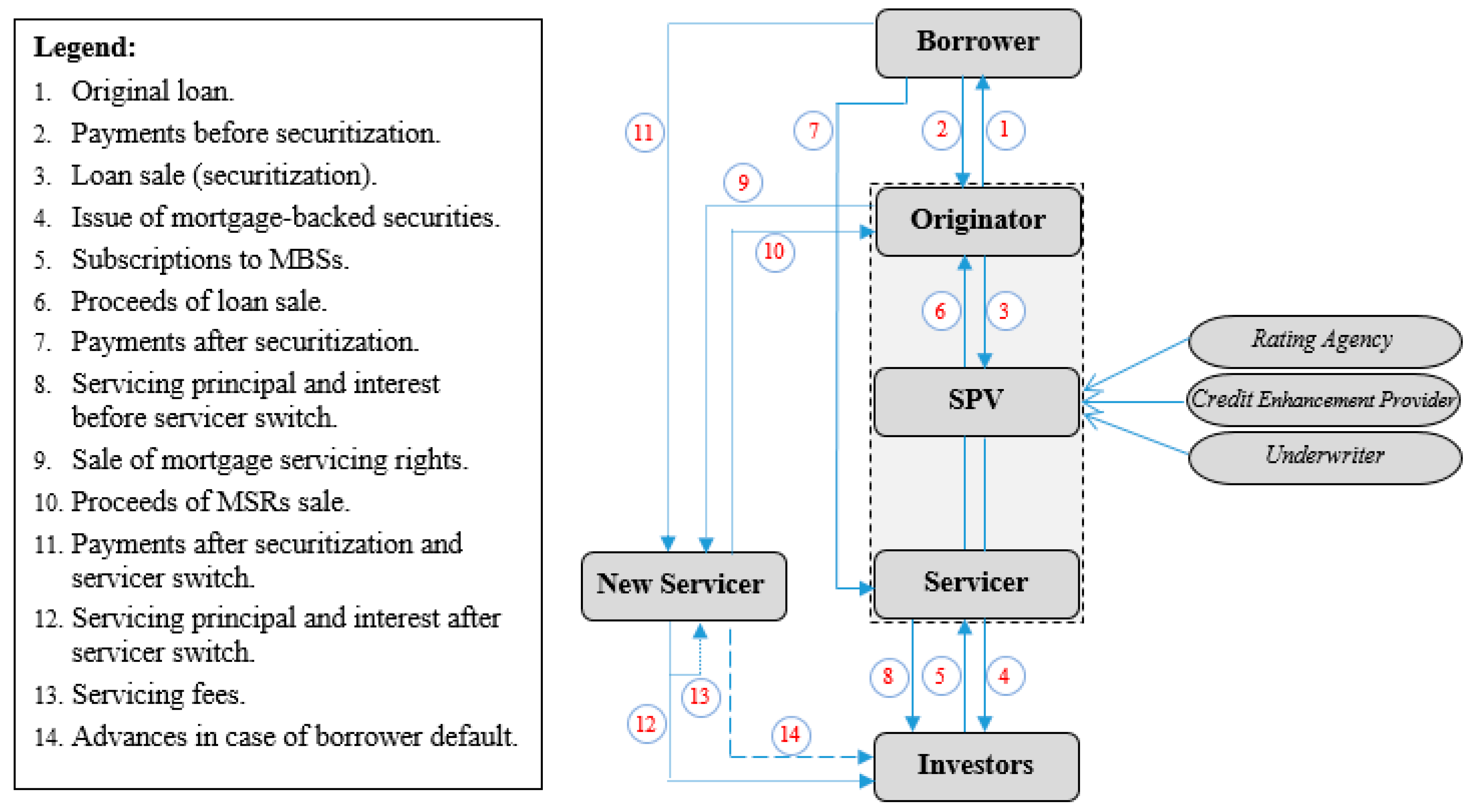
2.1. Representation of Mortgage Servicing Process

Figure 1 shows the various contracted parties involved in the mortgage servicing process along with the generated cash flows in every step. A typical mortgage lending process starts with a borrower applying for a mortgage in order to buy a property or to refinance an existing mortgage to take advantage of lower interest payments. Usually, the mortgage originator is a commercial bank, a credit union, or a non-depository retail lender. Whatever the case, the mortgage originator manages the complete loan-granting process. Based on its information set, the originating lender expends effort to assess the borrower’s reliability and creditworthiness. Eventually, if the borrower meets the lending requirements, the mortgage application is approved, and funds are released as represented by cash flow 1 in Figure 1. The debt payments in the absence of securitization are represented by cash flow 2.

This securitization is defined as the process whereby illiquid loans extended to borrowers are converted into liquid securities traded on financial markets. This process is summarized in steps 3 to 6. In the first step of the securitization process, the originating institution transfers the mortgage to a special purpose vehicle defined as a legally separate entity created to handle the securitization process. The mortgage transfer is marked by cash flow 3. This process of handling securitization involves external parties such as the underwriter that assists with the sale, the credit enhancement agency, and the credit rating agency that rates the interest-bearing securities. Once the tradable MBS are created and rated, the SPV sells them to investors, as depicted in cash flows 4 to 5. Finally, the SPV uses the proceeds of the MBSs sale to pay back the entity that originated the underlying debt, as illustrated by cash flow 6.

Once the securitization process is completed, the mortgage servicer ensures ongoing management and the upkeep of the payments. The main task of a mortgage servicer is collecting principal and interest payments from the borrower (cash flow 7) and passing the proceeds along to the underlying MBS investors in the secondary market (cash flow 8). Thus, as the borrower makes interest and principal payments, the servicer of the deal ensures that the cash flows are paid back to investors in accordance with the terms laid out in the securities prospectus. The mortgage originator can act as the servicer of the deal or it can sell the mortgage servicing rights (MSR) to a third party involved in this process, hereafter referred to as the new servicer or the MSR purchaser.

The sale of mortgage servicing rights and the corresponding cash proceeds are indicated by cash flows 9 and 10, respectively. In this case, the buyer of the mortgage servicing rights replaces the original servicer of the deal and ensures the ongoing mortgage management. Therefore, borrowers become directly linked to the new servicer to whom they continue making monthly debt payments (cash flow 11) that the former passes along to the MBS investors in the secondary market, as indicated by cash flow 12. Customarily, in return for these services, the new mortgage servicer is paid a monthly fee generally specified as a fixed percentage of the declining unpaid balance of the underlying mortgage loan. The new servicer is also entitled to collect other fees such as float income, late payment fees, and other ancillary income. All these income streams are represented by cash flow 13. Finally, if a delinquent borrower defaults on a loan and stops making monthly payments due to financial distress, the new mortgage servicer is required to advance funds to MBS investors in the secondary market in keeping with the terms and conditions of the loan servicing contract, as indicated by cash flow 14.

At this point, it is crucial to note that neither the new mortgage servicer nor MBS investors in the secondary market observe all the information that the originating lender possesses. In fact, information detained by the lender could be classified into two main forms: hard and soft (Agarwal and Hauswald 2010; Keys et al. 2010, 2012; Malekan and Dionne 2014; Agarwal and Ben-David 2018; Liberti and Petersen 2018, among others). Hard information includes quantitative records of data such as credit scores and financial records. Soft information includes information that cannot be quantified or stored such as opinions, and self-made judgments. In such an environment, the originating lender could (partially) provide hard information to a third party while soft information is privately held.

2.2. Cash Flows and Risks of the Servicer 1

The most important source of revenue for a mortgage servicer is the servicing fee, generally specified as a fixed percentage of the declining unpaid balance of the underlying mortgage. Servicers do not collect servicing fee revenue for non-performing loans for which borrowers are delinquent.

There are three main risks associated with the mortgage servicing activity: prepayment risk, default risk, and operational risk. The prepayment risk is defined as the possibility of an early, unscheduled, full repayment of the loan. The default risk is defined as the hazard that a borrower will be unable to honor the required principal and/or interest payments on the mortgage agreement in a timely manner. The risks due to the operational side of the servicing business are of an entirely different nature. For example, in servicing the deal, there is the possibility that the initial mortgage was made based on fraudulent information. In this study, we focus on the risk of borrower default.

3. The Nonparametric Estimation Framework

3.1. Motivation for Nonparametric Methods

The primary advantage of nonparametric estimation methods is robustness, as they can be applied in a broader range of situations even where the parametric conditions of validity are not met. Another notable advantage of nonparametric approaches is the ability to handle various data types (e.g., continuous, ordinal, and ranked data) even if the data comprise outliers, anomalies widely recognized to seriously affect the routine of parametric tests. Finally, as shown by Su and Spindler (2013), nonparametric tests may have stronger power than parametric tests.

Our empirical analysis considers the nonparametric kernel density estimation (KDE) technique to estimate the probability density function (PDF) of random variables drawn from unspecified probability distributions. Although we will assume that the distribution has a deterministic PDF, the estimation methodology will be entirely data-driven in the sense that data will be allowed to speak for themselves more than would be the case if the PDF were constrained to fall in a given parametric family.

3.2. Multivariate Kernel Density Estimation with Mixed Data Types

Consider a continuous random variable $X^c$ with a probability density function $f_{X^c}$. Let ${\left\{X_i^c\right\}}_{i=1}^n$ represents a sample of $n$ independent and identically distributed i.i.d. data points drawn from an unknown probability distribution family. Technically, a kernel $k(·)$ is defined as a function that weights sampled observations $X_i^c$ based on their distance from a specific evaluation point $x^c$ within a fixed range known as the bandwidth, $h$. The weights given by the kernel function to observations in the sample are known as local weights. The nonparametric estimator ${\widehat{f}}_{X^c}$ is commonly referred to as the Rosenblatt–Parzen estimator (Rosenblatt 1956; Parzen 1962).

For multivariate data under the i.i.d. assumption, the kernel-based estimator of the joint PDF is expressed as the product of univariate kernel functions. The considered approach uses the concept of “generalized product kernels” (Li and Racine 2007; Racine 2008). Accordingly, the estimator of the joint PDF of $q$ continuous variables can be written as follows:

$${\widehat{f}}_{X^c}\left(x_1^c,x_2^c,\dots ,x_q^c\right)={\displaystyle \frac{1}{n}}\sum _{i=1}^n\prod _{s=1}^q{\widehat{h}}_s^{-1}k\left({\displaystyle \frac{X_{i,s}^c-x_s^c}{{\widehat{h}}_s}}\right).$$

(1)

We use $X_{i,s}^c$ to denote the $s$-th component of the $q$-dimensional space of continuous regressors, where $s=\left\{1,\dots q\right\}$ and $i=\left\{1,\dots n\right\}$. ${\widehat{h}}_s$ refers to the estimated bandwidth of the $s$-th regressor. For the purpose of this paper, we consider the case where $X$ is a vector containing a mix of discrete and continuous variables. Let $X=(X^c,X^d)$ define the ensemble of $q$ continuous and $p$ discrete random variables. The joint density function for both categorical and continuous data using the generalized kernel product method can be formulated as follows:

$${\widehat{f}}_X\left(x_1^c,\dots ,x_q^c,x_1^d,\dots ,x_p^d\right)={\displaystyle \frac{1}{n}}\sum _{i=1}^n\prod _{s=1}^q{{\widehat{h}}_s}^{-1}k\left({\displaystyle \frac{X_{i,s}^c-x_s^c}{{\widehat{h}}_s}}\right)·\prod _{r=1}^{p}l\left(X_{i,r}^d,x_r^d,{\widehat{\gamma }}_r\right),$$

(2)

where $l\left(·\right)$ is a weighting kernel function that depends on the estimated bandwidth $\left(\widehat{\gamma }\right)$. $X_{i,r}^d$ denotes the $r$-th component of the $p$-dimensional space of discrete regressors, $r=\left\{1,\dots p\right\}$ and $i=\left\{1,\dots n\right\}$. The mixed-type kernel allows for having a nonparametric counterpart for discrete choice parametric models such as probit and logit.

3.3. Conditional Kernel Density Estimation for Information Asymmetry Test

The core of our information asymmetry test is the estimation of the conditional density function. Let $f_{Y|X}$ denotes the conditional density function of $Y$ given $X$. Since our dependent variable $Y$ is discrete, the conditional kernel-based estimator is given by:

$${\widehat{f}}_{Y|X}\left(y|x^c,x^d\right)={\displaystyle \frac{\frac{1}{n}\sum _{i=1}^{n}K\left(X_i^c,x^c\right)·L\left(X_i^d,x^d\right)·l\left(Y_i,y,{\widehat{\gamma }}_y\right)}{\frac{1}{n}\sum _{i=1}^{n}K\left(X_i^c,x^c\right)·L\left(X_i^d,x^d\right)}},$$

(3)

where, for expositional simplicity, $K\left(X_i^c,x^c\right)=\prod _{s=1}^q{\widehat{h}}_s^{-1}k\left({\displaystyle \frac{X_{i,s}^c-x_s^c}{{\widehat{h}}_s}}\right)$ denotes the standard product kernel of $s$ continuous variables. Similarly, $L\left(X_i^d,x^d\right)=\prod _{r=1}^{p}l\left(X_{i,r}^d,x_r^d,{\widehat{\gamma }}_r\right)$ denotes the product kernel functions of $r$ discrete variables. Note that $x^c$ and $x^d$ are $p\times 1$ and $q\times 1$ vectors of evaluation points, respectively. $l\left(Y_i,y,{\widehat{\gamma }}_y\right)$ denotes the univariate kernel density estimator for discrete variable $Y$ with an estimated bandwidth ${\widehat{\gamma }}_y$. For the purpose of the information asymmetry testing procedure, our object of interest is the cumulative distribution function (CDF) estimated by the kernel-based density estimation approach. Let $F_{Y|X}$ denotes the conditional CDF of $Y$ given $X$. A nonparametric estimate of $F_{Y|X}$ is given by the following expression:

$${\widehat{F}}_{Y|X}\left(y|x^c,x^d\right)={\displaystyle \frac{\frac{1}{n}\sum _{i=1}^{n}K\left(X_i^c,x^c\right)·L\left(X_i^d,x^d\right)·I\left(Y_i\le y\right)}{\frac{1}{n}\sum _{i=1}^{n}K\left(X_i^c,x^c\right)·L\left(X_i^d,x^d\right)}},$$

(4)

where $I\left(Y_i\le y\right)$ denotes an indicator function. This equation represents the core of the nonparametric test proposed by Su and Spindler (2013). In Section 4, we provide a detailed description of the testing procedure along with the hypothesis to be tested. The estimated value for the bandwidth (denoted $\widehat{h}$ for the continuous variable kernel and $\widehat{\gamma }$ for the discrete variable kernel) is the value minimizing the integrated mean square error, or IMSE, simply defined as a measure of the discrepancy between the estimated density ${\widehat{f}}_h$ and the true density f:

$$\begin{array}{ll}{IMSE}_{{\widehat{f}}_h\left(x\right)}& =E\left\{\int {\left({\widehat{f}}_h\left(y\right)-f\left(y\right)\right)}^{2}dy\right\}\\ & =\int {Biais\left({\widehat{f}}_h\left(y\right)\right)}^{2}dy+\int Var\left({\widehat{f}}_h\left(y\right)\right)dy.\end{array}$$

(5)

The optimal bandwidth is a function of the second derivative of the true density, which is unknown in the model. The bandwidth approximation methods use some underlying assumptions about the true density, which are useful in an application with a large number of variables or a large sample size, as in our empirical application.

4. Nonparametric Information Asymmetry Test

We want to test if the data contains residual asymmetric information effects in the relationship between mortgage default and the decision to use a new servicer. We hypothesize that their informational advantage influences the behavior of mortgage originators by selling mortgage servicing rights. Formally, let $Y$ denote the dependent variable or outcome, $X$ the set of exogenous control variables, and $Z$ a decision variable. In our context of mortgage servicing, $Y$ refers to the event of default mortgage, $X$ includes mortgage risk characteristics and borrower credit quality variables that are observable by both parties (hard information), while $Z$ denotes the originator’s decision to sell the mortgage servicing rights rather than to keep servicing. In a principal-agent context, the decision variable, $Z$, should provide no useful information on mortgage default if and only if the prediction of $F\left(Y\right)$ given $X$ and $Z$ jointly coincides with its prediction given $X$ alone (Dionne et al. 2001, 2006). If this is the case, the information asymmetry hypothesis is rejected. The above statement could be formally written in terms of conditional probability functions:

$$F\left(Y/X,Z\right)=F\left(Y/X\right),$$

(6)

where $F\left(Y/X,Z\right)$ denotes the conditional cumulative density function (CDF) of mortgage default. Equation (6) means that the original lender’s action to switch the servicer or to continue servicing the deal does not convey any additional information useful in predicting the probability of default of a given mortgage as long as all loan and borrower observable risk characteristics (hard information) reveal all necessary information to compute the CDF of mortgage default.

Given a set of $n$ i.i.d. randomly drawn observations ${\{Y_i,Z_i,X_i^c,X_i^d\}}_{i=1}^n$, the nonparametric test is resumed in comparing the following two conditional CDF estimates $\widehat{F}\left(y|x^c,x^d,z=1\right)$ and $\widehat{F}\left(y|x^c,x^d,z=0\right)$ as presented in Equation (4) but augmented by the decision variable Z as follows:

$$\widehat{F}\left(y|x^c,x^d,z\right)={\displaystyle \frac{\frac{1}{n}\sum _{i=1}^{n}K\left(X_i^c,x^c\right)·L\left(X_i^d,x^d\right)·I\left(Y_i\le y\right)·I\left(Z_i=z\right)}{\frac{1}{n}\sum _{i=1}^{n}K\left(X_i^c,x^c\right)·L\left(X_i^d,x^d\right)·I\left(Z_i=z\right)}}.$$

(7)

A test statistic measures the variation in $\widehat{F}\left(y|x^c,x^d,z\right)$ across possible values of $z$ and different observations as follows:

$$D^{*}=\sum _{i=1}^n{\left[\widehat{F}\left(y_i|x_i^c,x_i^d,z_i=1\right)-\widehat{F}\left(y_i|x_i^c,x_i^d,z_i=0\right)\right]}^2·a\left(x_i^c\right),$$

(8)

where $a(·)$ is a uniformly bounded nonnegative weight function with compact support that lies within the support of $X_i^c$. This quantity serves to perform trimming in areas of sparse support of the continuous conditioning variable. It can be formulated as follows:

$$a\left(x_i^c\right)=\prod _{s=1}^{q}I\left(q_s\left(0.025\right)\le X_{i,s}^c\le q_s\left(0.975\right)\right),$$

(9)

where $q_s\left(\alpha \right)$ denotes the $\alpha$-$\mathrm{t}\mathrm{h}$ sample quantile of the $s$-$\mathrm{t}\mathrm{h}$ component of $X_i^c$ and $q$ is the total number of continuous variables. The test statistic $D^{\mathrm{*}}$ in Equation (8) could be viewed as the difference between the expected probability of default depending on whether the originator switches the servicer or not. We can show that $D^{\mathrm{*}}$ is asymptotically normally distributed under the null hypothesis of independence. We implement a bootstrap procedure to obtain the corresponding p-values. In Section 6.3, we propose an extension of the test in order to consider a causal relationship between Z and Y.

5. Data, Variables, and Summary Statistics

5.1. Data Source and Sample Construction

To empirically test for asymmetric information in the mortgage servicing market, we use a large data set provided by MBSData, LLC, River Edge NJ. The data comprise U.S. mortgages that were securitized through the non-agency channel. Mortgages securitized through the private-label channel have fundamental risk characteristics that make them riskier than average. In general, mortgages securitized through this channel do not conform to the prudent lending guidelines set by the government-sponsored enterprises (GSE) Freddie Mac, Fannie Mae, and Ginnie Mae. For example, most of the mortgages do not meet the GSE requirements in terms of loan size (e.g., jumbo loans with original loan amounts exceeding the conforming loan limits), documentation (e.g., loans with no or low level of documentation), and loan-to-value ratios (e.g., LTV ratio above 80%).

Owing to the lack of a government guarantee, holding these private-label securities carries a significantly higher risk than carrying the agency counterparts. For instance, without government back-up, private-label mortgage originators rely on both credit rating agencies and credit enhancements to attract MBS investors and convince them that the underlying mortgage is safe. The non-agency market had witnessed tremendous growth during the pre-crisis period. For instance, the outstanding quantity of non-agency mortgages grew from roughly $600 billion at the end of 2003 to $2.2 trillion at its peak in 2007, according to JP Morgan. The bad risk management of this tremendous growth in the non-agency market is widely recognized by both researchers and practitioners as being one of the main triggers of the financial crisis.

Our dataset consists of mortgages issued between January 2000 and December 2013. The initial sample consists of more than 25 million mortgages that were originated throughout the U.S. and granted by diverse types of lenders ranging from top investment banks to regional small retailers. The yearly distribution of loan origination follows a pattern similar to that observed in the entire U.S. mortgage market. The MBSData, LLC database consists of two main datasets. The first static file reports detailed information collected at the time of mortgage origination. For instance, it reports the borrower’s FICO credit score, loan-to-value (LTV) ratio, loan purpose, payment type, initial interest rate, private insurance coverage, etc. It also provides information regarding the property backing the loan, which includes the house value, state, city, and zip code. For the originating entity, the database reports the originating lender’s name and type, the name of the original mortgage servicer, as well as the most recently updated servicer name. The second dynamic file reports information that has been collected over the loan lifetime on a monthly basis. Key variables recorded in the monthly remittance files are the current loan balance, current interest rate, next due date, and a monthly delinquency code (current, paid-off, +30, +60, or +90 days delinquent, in foreclosure, in bankruptcy, or real estate owned). The dataset also provides information on losses and loan modification. Loss files mainly report loan-level loss amount, loss severity, recovery amount, loan liquidation proceeds, and current value at liquidation.

While constructing our sample, we impose several restrictions in order to create a homogenous loan sample. We focus on mortgages in a first-lien position on the property securing the mortgage and exclude second mortgages and home equity lines of credit (HELOCs). Our choice is primarily motivated by the fact that first-lien mortgages have priority over all other subsequent claims (i.e., second-lien or junior) on a property in the event of borrower default. We restrict our attention to single-family owner-occupied homes and exclude multifamily and/or non-owner occupied properties. We also exclude loans whose main purpose is designated as home improvement and retain loans with the main purpose identified as a house purchase or refinancing an existing mortgage (both cash-out and no cash-out). We also exclude planned unit developments (PUDs) and mobile homes. All these restrictions result in a final sample including 5,591,353 distinct observations that originated between January 2000 and December 2013 and were tracked until December 2015 on a monthly basis.

5.2. Variables and Hypotheses

The main variable of interest in our empirical analysis is the mortgage servicer switching indicator, denoted as Switch_Servicer. This variable is a dummy indicator that equals 1 if the originating lender sells the mortgage servicing right to another servicer and 0 if the lender continues servicing the mortgage it originates. The second most important variable of interest is the standard Default dummy variable, which denotes whether a given mortgage becomes 90+ days delinquent (i.e., when a loan is first reported as the borrower having missed three or more consecutive monthly payments). For robustness, we also report results with 60+ days delinquent in the online Appendix A.

The set of covariates includes several explanatory variables recorded at the time of origination. All variables are defined in

Table A1. Variable definition and source.

Name	Type	Description	Source
Switch Servicer	Binary	Denotes the decision of the originating lender to sell or to retain the mortgage servicing right of a given loan. Takes the value of 1 if the originator decides to sell the underlying MSR and 0 if he retains the MSR and continues servicing the loan.	MBSData
Default	Binary	Denotes mortgage default. Takes the value of 1 if the borrower of a given mortgage misses three or more consecutive monthly payments (i.e., when the mortgage status is first labeled as 90+ days delinquent).	MBSData
FICO score	Continuous	The borrower’s FICO score created and calculated by the Fair Isaac Corporation. It measures the credit quality of borrowers by taking into account an individual’s payment history, length of credit history, current level of indebtedness, and types of credit used by the borrower.	MBSData
FICO660	Binary	Takes the value of 1 if the borrower’s FICO score is above 660 and 0 otherwise. In general, a FICO score above 660 indicates that the individual has a good credit history.	MBSData
LTV	Continuous	The loan-to-value ratio calculated as the percentage of the first-lien mortgage to the total value of the property. It is one of the key risk factors used by U.S. lenders when qualifying borrowers for a mortgage. A high LTV ratio mirrors a loan with a low down payment for which the borrower has little equity stake in the property.	MBSData
LTV80	Binary	Takes the value of 1 if the LTV ratio is equal to or higher than 80%.	MBSData
DTI	Continuous	The debt-to-income ratio calculated as the fraction of monthly mortgage payments to the borrower’s monthly income. DTI measures the borrower’s ability to honor periodic debt payments as it compares debt payments to the borrower’s income.	MBSData
No/Low doc.	Binary	Takes the value of 1 if the documentation level is labelled “missing” or “low”, and 0 otherwise. No- or low documentation mortgages designate loans for which the lender did not gather a sufficient level of information on the borrower’s reliability and credit worthiness.	MBSData
ln Amount	Continuous	The natural logarithm of the initial balance of the mortgage. Does not include either interest, taxes, or fees.	MBSData
Interest	Continuous	The interest rate was initially applied at the time of original underwriting. Higher interest rates usually reflect loans granted to borrowers with inferior credit quality, which increase their monthly debt payments.	MBSData
ARM	Binary	Takes the value of 1 if the loan type is an adjustable-rate mortgage and 0 if fixed-rate mortgage. ARM indicates whether the interest rate of a given mortgage is fluctuating over time based on a benchmark index plus an additional spread, called an ARM margin.	MBSData
ARM margin	Continuous	A fixed component added to the interest rate for ARM mortgages. The margin is constant throughout the lifetime of the mortgage, while the benchmark index fluctuates over time according to general market conditions.	MBSData
Balloon	Binary	Takes the value of 1 if the mortgage has a balloon payment structure, 0 otherwise. Balloon mortgagors make only interest payments during the lifetime of the loan. At the term end, the borrower repays the entire principal at once.	MBSData
GSE conforming	Binary	Takes the value of 1 if the lender follows the GSEs’ lending guidelines and 0 otherwise. Following the GSEs’ recommendations, we classify a mortgage as conforming if the borrower’s FICO score is above 660 and the loan amount is below the conforming loan limit in place at the time of origination and the LTV is either less than 80% or the loan has private mortgage insurance in the case that the LTV ratio is above 80%. Since conforming loans meet the GSE lending standards, the conforming dummy variable indicates whether the mortgage was eligible to be sold to the GSEs at origination.	MBSData
Subprime	Binary	Denotes subprime mortgages. A mortgage is labelled “Subprime” at origination if the borrower’s FICO score is lower than 580 or the LTV ratio is higher than 90%.	MBSData
Prime	Binary	Denotes prime mortgages. A mortgage is considered as “Prime” if the borrower’s FICO score is higher than 660 and the LTV ratio is lower than 80%.	MBSData
Prep. Penalty	Binary	Equals to 1 if the mortgage contract includes a prepayment penalty clause and 0 otherwise. Accordingly, the borrower will pay a penalty if he chooses to pre-pay the loan within a certain time period. The penalty is based on the remaining mortgage balance and the number of months worth of interest.	MBSData
Purchase	Binary	Takes the value of 1 if the loan purpose is labeled “Purchase” a property and 0 otherwise.	MBSData
Refin. cash-out	Binary	Equals to 1 if the loan is granted for the purpose of refinancing an existing loan with “cash-out”. A cash-out refinance mortgage is a new loan in which the amount is greater than the existing mortgage amount, which will be refinanced. Since the borrower refinances for more than the amount owed, he/she takes the difference in cash.	MBSData
Refin. no cash-out	Binary	Equals to 1 if the loan is granted for the purpose of refinancing an existing loan with “no-cash-out”. A no-cash-out refinance mortgage is a new loan in which the amount is equal to or lower than the existing mortgage amount. The main purpose of such loans is usually to lower the interest rate charge on the loan.	MBSData
Service fee	Continuous	The servicing fee that the servicer of the deal charges as compensation for costs he bears. It is expressed as a fixed percentage of the declining balance of the mortgage.	MBSData
Age at default	Continuous	The age-at-default is measured as the total number of months since origination when the default is first recorded.	MBSData
Default N	Binary	Denoting the fraction of mortgages that default within N months since origination.	MBSData
Income	Continuous	The annual growth rate of personal income, which is defined as an individual’s total earnings from wages, investment interest, and other sources. The seasonally unadjusted U.S. real disposable (after deducting tax) personal income data is retrieved from the US. Bureau of Economic Analysis’ web site.	bea.gov
Divorce	Continuous	The annual divorce rate calculated as the ratio of the number of marriages contracted and ended in divorce to the number of all marriages contracted in the same year. The divorce rate is commonly used as an indicator of social stress in the society. The seasonally unadjusted divorce rate is retrieved from the U.S. Census Bureau’s web site.	census.gov
GDP growth	Continuous	The annual growth rate of the U.S. Real Gross Domestic Product. The real GDP is collected from the Federal Reserve Bank of St. Louis’ web site.	stlouisfed.org
HPI growth	Continuous	The annual growth rate of the House Price Index for the U.S. We use the seasonally unadjusted purchase-only HPI index retrieved from the Federal Reserve Bank of St. Louis’ web site.	stlouisfed.org
σ interest	Continuous	The interest rate volatility calculated as the volatility on the 1-Year Treasury Constant Maturity Rate over the 24 months before origination. The monthly seasonally unadjusted treasury rate is collected from the Federal Reserve Bank of St. Louis’ web site.	stlouisfed.org
Credit spread	Continuous	The yield spread between AAA and Baa bond indexes. It is calculated as the interest rate difference between Moody’s Aaa and Baa Corporate Bond Yields. Both variables are seasonally unadjusted, recorded on a monthly basis, and retrieved from the Federal Reserve Bank of St. Louis’ web site.	stlouisfed.org
Judicial	Binary	Takes the value of 1 if the state laws require judicial procedures to foreclose on a mortgage and 0 if not. The variable is compiled based on information from the National Center for State Courts’ web site.	ncsc.org
SRR	Binary	Stands for Statutory Right of Redemption and takes the value of 1 if the state has statutory redemption laws. The variable is compiled based on information from the National Center for State Courts’ web site.	ncsc.org

of the online Appendix A. The first variable we consider is the borrower’s FICO score. In general, the FICO score measures individuals’ creditworthiness by taking into account their payment history, length of credit history, current level of indebtedness, and types of credit used. The score ranges from 300 to 850, and, typically, a FICO score above 660 is indicative of a good credit history. We expect that the originator will keep servicing mortgages with high FICO scores.

The second independent variable is the loan-to-value ratio, LTV, calculated by lenders as the percentage of the first-lien mortgage to the total appraised value of the purchased property. The LTV ratio is one of the key risk factors used by U.S. lenders when qualifying borrowers for a mortgage. In the United States, mortgagors with LTV ratios higher than 80% are required to buy private mortgage insurance to protect the lender from the default risk, which increases the cost of borrowing. The LTV ratio also measures the equity stake of borrowers in a given property. The higher the LTV ratio, the lower the down payment, so the lower the borrower’s equity stake in that house. Since a high LTV ratio mirrors a risky mortgage, where the borrower holds a lower equity stake in a given house, we expect the lender’s decision to switch the servicer of the deal will be positively correlated with the LTV ratio.

Another key explanatory variable in our analysis is no/low documentation, a dummy variable indicating whether the lender has collected the required level of documentation on the borrower. Typically, a borrower is asked to fill out a credit application and provide several statements and proofs of employment status and income when applying for a loan. Based on this documentation, the lender expends effort to assess the borrower’s creditworthiness. Therefore, a no/low documentation loan is a loan for which the lender has not gathered a sufficient level of information on the borrower’s income. In terms of default risk, we can presume that no/low documentation loans will default more frequently.

The next independent variable is the ARM indicator; ARM stands for adjustable-rate mortgages (commonly referred to as variable-rate mortgages). The ARM variable indicates whether the interest rate paid on the outstanding balance of a given mortgage varies according to a specific benchmark. Usually, the initial interest rate is fixed for a period of time, after which it is reset periodically, often every month. The interest rate paid by the borrower is usually based on a benchmark plus an additional spread, called the ARM margin. In terms of risk, ARM-type mortgages transfer part of the interest-rate risk from the lender to the borrower. Indeed, these mortgages are generally used when interest rates fluctuate and are difficult to predict (which makes fixed-rate mortgages, FRMs, difficult to obtain). In terms of servicing choice, a positive statistical relationship is expected between terms of servicing choice and interest rate.

We also include a GSE conforming indicator to denote loans that obey the GSEs’ lending guidelines. The GSE_conforming dummy variable indicates whether the mortgage was eligible to be sold to the GSEs at origination. Following the GSEs’ recommendations, we classify a mortgage as conforming if the borrower’s FICO score is above 660 and the loan amount is below the conforming loan limit in place at the time of origination and the LTV is either less than 80 percent or the loan has private mortgage insurance if the LTV is greater than 80 percent. Given that conforming loans meet the GSE lending standards, we expect a negative correlation with the default event. Indeed, falling within the GSE prudence guidelines should significantly reduce the probability of default. Regarding the choice of switching the servicer, we presume that both signs are plausible. On the one hand, being GSE-conforming increases the ease of finding a buyer of the underlying MSRs. For instance, because these loans are originated following the GSE standards, it would be easier to find buyers of the securitized pool of loans in the market. Thus, a positive sign is expected. On the other hand, being GSE-conforming increases the probability that the lender will be paid back as scheduled. Lenders may therefore keep these good-quality loans on their balance sheets because the risk of default on these loans is significantly low. Therefore, the sign of the conforming coefficient is an empirical matter.

5.3. Descriptive Statistics

We start the empirical analysis by providing summary statistics of some of the key variables used in our analysis. Since we are focusing on the non-agency market, we pay special attention to the role of credit scores, loan-to-value ratios, the amount of documentation collected by the lender, and some interest rate features.

Table A2. Summary statistics by origination year. The table reports summary statistics for the sample of U.S. mortgages originated over the period from January 2000 to December 2013. The mortgages have been securitized through the non-agency channel. The first row reports statistics over the 2000–2013 study period for the total sample of 5,591,353 distinct mortgages, while the next rows report statistics by origination year. The first two columns, Volume (in %) and Volume (in $B), refer to the total origination volume expressed in percentage of the total sample and in US$ billions, respectively. FICO score abbreviates the borrower’s Fair Isaac Corporation score attributed at origination. FICO.660 denotes the fraction of loans granted to borrowers with FICO scores higher than 660. LTV abbreviates the initial loan-to-value ratio. LTV.80 denotes the fraction of loans with LTV ratios higher than 80%. DTI stands for the debt-to-income ratio. No/Low doc. indicates whether the originator collected either no or low documentation. Interest rate is the coupon rate applied at origination. Balloon denotes balloon payment mortgages. ARM and ARM margin denote adjustable-rate mortgages and the corresponding margin. GSE conf. denotes the fraction of loans that conform to the Government-Sponsored Enterprises’ prudent lending guidelines. Prep. Penalty measures the fraction of loans with prepayment penalties.

Origination Year	Volume (in %)	Volume (in $B)	FICO Score	FICO. 660	LTV Ratio	LTV. 80	DTI	No/Low Doc.	Interest Rate	Balloon	ARM	ARM Margin	GSE Conf.	Prep. Penalty
All period	100.0	1509.1	657.12	0.48	76.93	0.60	38.65	0.47	6.97	0.06	0.63	5.00	0.17	0.49
2000	1.05	8.87	615.49	0.31	78.20	0.62	38.65	0.34	10.08	0.07	0.34	6.13	0.17	0.41
2001	2.47	32.07	648.33	0.47	76.87	0.56	37.74	0.29	8.56	0.03	0.36	6.09	0.23	0.33
2002	5.74	69.08	644.97	0.42	77.47	0.58	37.84	0.33	7.92	0.02	0.54	5.92	0.21	0.38
2003	11.46	170.89	670.12	0.56	75.14	0.51	36.95	0.38	6.60	0.01	0.49	5.18	0.25	0.31
2004	16.93	232.68	657.75	0.49	77.60	0.60	36.81	0.44	6.30	0.00	0.70	4.75	0.19	0.52
2005	27.28	411.36	658.81	0.49	76.97	0.62	38.33	0.51	6.51	0.02	0.69	4.91	0.16	0.53
2006	27.11	422.92	650.45	0.44	77.44	0.63	39.90	0.52	7.44	0.15	0.66	5.07	0.12	0.57
2007	7.79	153.39	668.92	0.56	75.92	0.56	39.17	0.57	7.32	0.12	0.52	4.50	0.15	0.47
2008	0.02	0.60	717.06	0.80	73.25	0.44	36.59	0.40	7.16	0.03	0.48	3.13	0.03	0.17
2009	0.00	0.21	774.60	1.00	53.11	0.06	36.00	0.30	4.79	0.00	0.83	2.04	0.03	0.00
2010	0.01	0.43	772.33	1.00	61.78	0.17	32.48	0.02	4.93	0.00	0.08	1.64	0.01	0.21
2011	0.02	1.17	770.62	1.00	66.60	0.23	32.98	0.17	4.72	0.00	0.06	1.83	0.01	0.16
2012	0.06	2.79	773.08	1.00	66.42	0.20	34.00	0.03	4.06	0.00	0.02	2.25	0.00	0.13
2013	0.06	2.67	771.14	1.00	66.24	0.19	30.80	0.00	3.91	0.00	0.01	2.53	0.00	0.01

reports descriptive statistics over the entire study period from January 2000 to December 2013 as well as segmented by origination year.

Table A3. Summary statistics by loan type and status. The table reports summary statistics for the sample of 5,591,353 U.S. mortgages originated over the period from January 2000 to December 2013. The mortgages have been securitized through the non-agency channel. The table breaks down the sample by payment type (FRM vs. ARM), loan type (prime vs. subprime), financial crisis era (before vs. after), default status, and servicer switch status. FICO score abbreviates the borrower’s Fair Isaac Corporation score at origination. FICO.660 denotes the fraction of loans granted to borrowers with a FICO score higher than 660. LTV abbreviates the initial loan-to-value ratio. LTV.80 denotes the fraction of loans with LTV ratios greater than 80%. DTI stands for the debt-to-income ratio. No/Low doc. indicates whether the originator collected either no or low documentation. Interest rate is the coupon rate applied at origination. Balloon denotes balloon payment mortgages. ARM and ARM margin denote adjustable-rate mortgages and the corresponding margin. Subprime and prime are subprime loan classifiers. GSE conf. denotes the fraction of loans conforming to the GSEs’ lending guidelines. Prep. Penalty indicates the fraction of mortgages with a prepayment penalty. Service fee is the mortgage servicer fee expressed as a percentage of the remaining balance. Switch servicer indicates the fraction of mortgages for which the originator switched the servicer of the deal. Default denotes the fraction of mortgages in default. Age at default is the average age of defaulting mortgages. Default 12, Default 18, and Default 24 refer to the fraction of loans defaulting within 12, 18, and 24 months since origination, respectively.

	All	Payment Type		Loan Type		Financial Crisis		Default		Switch Servicer
		FRM	ARM	Prime	Subprime	Before	After	No	Yes	No	Yes
FICO score	657.12	678.00	644.84	730.93	634.87	655.92	671.02	669.62	635.77	660.62	654.23
FICO.660	0.48	0.61	0.41	1.00	0.33	0.48	0.57	0.55	0.37	0.51	0.46
LTV	76.93	73.89	78.73	63.48	80.99	77.04	75.72	74.86	80.48	76.49	77.30
LTV.80	0.60	0.48	0.67	0.00	0.78	0.60	0.55	0.53	0.72	0.58	0.61
DTI	38.65	37.64	39.08	35.71	39.10	38.60	39.09	37.63	39.91	38.02	38.95
No/Low doc.	0.47	0.46	0.48	0.63	0.43	0.46	0.55	0.45	0.50	0.49	0.45
Interest rate	6.97	7.10	6.89	5.57	7.39	6.94	7.26	6.71	7.41	6.86	7.05
Balloon	0.06	0.04	0.08	0.01	0.08	0.06	0.12	0.03	0.11	0.04	0.08
ARM	0.63	0.00	1.00	0.45	0.68	0.64	0.52	0.59	0.70	0.59	0.66
ARM margin	5.00	.	5.00	2.86	5.42	5.03	4.50	4.80	5.27	4.93	5.04
Subprime	0.77	0.66	0.83	0.00	1.00	0.77	0.72	0.70	0.89	0.75	0.78
Prime	0.23	0.34	0.17	1.00	0.00	0.23	0.28	0.30	0.11	0.25	0.22
GSE Conf.	0.17	0.25	0.12	0.56	0.05	0.17	0.15	0.21	0.10	0.19	0.15
Prep. Penalty	0.49	0.34	0.58	0.24	0.57	0.50	0.46	0.42	0.63	0.49	0.50
Purchase	0.37	0.30	0.42	0.22	0.42	0.38	0.30	0.36	0.40	0.36	0.39
Refin. cash-out	0.47	0.49	0.45	0.46	0.47	0.46	0.51	0.46	0.47	0.49	0.45
Refin. no cash-out	0.16	0.21	0.13	0.31	0.11	0.15	0.19	0.18	0.12	0.15	0.16
Service fee	0.44	0.38	0.47	0.33	0.47	0.44	0.39	0.42	0.46	0.41	0.46
Switch servicer	0.55	0.50	0.58	0.52	0.56	0.56	0.44	0.18	0.50	0.00	1.00
Default	0.37	0.30	0.41	0.18	0.43	0.35	0.54	0.00	1.00	0.26	0.62
Age at default	36.64	45.25	32.98	47.72	35.21	37.41	30.81	.	36.64	38.07	35.47
Default 12	0.11	0.06	0.12	0.03	0.12	0.10	0.12	.	0.11	0.09	0.12
Default 18	0.23	0.15	0.26	0.08	0.24	0.22	0.26	.	0.23	0.20	0.24
Default 24	0.35	0.24	0.40	0.15	0.38	0.34	0.44	.	0.35	0.32	0.37

breaks down the sample by payment type (FRM vs. ARM), loan type (prime vs. subprime), before/after financial crisis, default status, and servicer switch status.

The first two columns of Table A2 provide a comprehensive picture of the evolution of the non-agency segment of the mortgage market over the 14-year study period. At first glance, mortgage origination has witnessed two major trends explained by the financial crisis. First, the market expanded rapidly from 2000 to 2006 and reached its highest level just before the financial crisis. Afterwards, mortgage origination plunged dramatically. During 2008 and 2009, the market also sustained a dramatic drop in origination of new mortgages. After the financial crisis (2010 and beyond), origination increased slightly but remained far from its level before the financial crisis.

The third column of Table A2 displays the average FICO credit score in the sample. The average credit score is 4 points lower than the 660 threshold. The evolution of the FICO credit score over the years is interesting. For instance, borrowers’ credit quality was below the 660 threshold before the financial crisis (655) but above it afterwards (671). The credit score averaged 615 and 644 in years 2000 and 2002. However, after the crisis, credit quality improved significantly as the average FICO score is consistently higher than 770 in the 2010–2013 period.

Figure A1 and Figure A2 of the online Appendix A examine the evolution of borrowers’ credit quality. They depict the evolution of FICO scores by payment type (ARMs vs. FRMs) and by loan type (prime vs. subprime). As shown in Figure A1, ARM borrowers have lower credit scores than FRM borrowers, on average. For example, in 2002, the average FICO scores for ARMs and FRMs were 619 and 672, respectively. This trend is almost verified for the period before the financial crisis, after which the difference in credit scores is reduced to 10 points. Table A3 shows that the ARM-FRM FICO score differential over the study period is about 34 points, statistically significant at the 1% level. Figure A2 suggests that, unsurprisingly, the average credit score for subprime loans is significantly lower than for prime loans. For illustration, in 2002 the average FICO score for subprime loans is almost 120 points lower than for prime borrowers (616 versus 735). Table A3 indicates that over the study period, the average FICO scores for prime and subprime borrowers are 731 and 635, respectively. The difference of 96 FICO points is statistically significant at the 5% level. After the financial crisis, the average credit score tended to improve each year, mainly due to the drop in subprime lending. As column 4 of Table A2 indicates, almost all loans originated after the financial crisis have a credit score higher than 660.

Regarding the loan-to-value (LTV) ratio of sampled mortgages, columns 5 and 6 of Table A2 show that the average LTV ratio in the sample is 77% and that 60% of loans in the sample have an LTV ratio higher than 80%. Regarding the evolution of the LTV ratio over the years, the LTV ratio plunged significantly soon after the financial crisis. For instance, column 6 of Table A2 shows that more than 60% of loans have an LTV ratio higher than 80% throughout the pre-crisis period. However, this proportion drops to almost 20% in the 2010–2013 post-crisis period. We further split our sample according to payment type (ARMs versus FRMs) and loan type (prime versus subprime). Table A3 shows the results over the entire studied period.

We also investigate the lender’s effort to gather all documentation required at the date of original underwriting. The statistics show that lenders did not gather sufficient documentation on applicants in almost half of the cases (47% of the time, lenders granted funding to borrowers but gathered little or no documentation on borrowers’ income and employment status). Yearly statistics show that this practice of granting funding without the required documentation increased steadily in the early 2000s. As shown in Figure A3, the high proportion of no/low documentation is mainly driven by the practice in the subprime segment; this proportion peaked at 70% from 2005 through 2007.

In general, the lending strategy appears to radically change after the financial crisis. This shift in lending strategy entailed (i) increasing loans granted for borrowers with good credit quality, (ii) reducing loans with a small down payment (LTV ratio higher than 80%), and (iii) reducing the proportion of loans granted with insufficient documentation. These changes in underwriting patterns are consistent with lenders looking for new ways to limit risk exposure after the financial crisis.

To motivate our empirical analysis, we contrast the ex-ante risk characteristics of mortgages for which the originator chooses to sell the underlying servicing rights to another servicer with mortgages that it chooses to continue to service. Overall, we note that, for 54.7 percent of the sampled mortgages (3,060,083 mortgages), the originator chooses to switch the mortgage servicer. For the remaining loans (45% of the sample), the originator keeps servicing mortgages it originates and holds them in its servicing portfolio until maturity. Table A3 shows that the average servicing fee is 44 bp, which does not change very much before and after the crisis. On average, lenders in the sample tend to charge significantly higher fees than the average servicing fees applied by the GSEs and the FHA/VA, at 25 bp and 19 bp, respectively.

Regarding the borrower’s credit quality, the results show that lenders tend to keep servicing loans granted to borrowers with superior credit quality. For illustration, the average credit score for loans held in the originator’s servicing portfolio is 661, while the average credit score for loans for which the lender decides to switch servicing is 654, namely 3 basis points below the sample average. The two-sample mean difference (untabulated) is 6.39 points, statistically significant at the 1% level. Table A3 also shows that the fraction of loans granted for borrowers with FICO scores higher than the 660 threshold is significantly larger for loans held in a portfolio (51% for non-switch versus 46% for switch).

These results indicate that lenders switch servicing of the deal for loans that are riskier and keep servicing mortgages that are less risky. For instance, the pool of loans for which the servicer has changed is characterized by higher loan-to-value ratios and slightly higher debt-to-income ratios. Regarding the subprime loan type, the primary statistics are not informative in that the propensity to switch the servicer of the deal is 52% for prime loans and slightly higher, at 56%, for subprime loans. The results also suggest that 15% of loans for which the servicer is switched follow the GSEs’ prudent lending guidelines, whereas this percentage increases to 20% for loans held in the originator’s servicing portfolio. The proportion of loans that conform to the GSE lending guidelines at origination represents only 17% of the sample.

To summarize, based on the observable risk characteristics of originated mortgages, these preliminary results are consistent with the evidence of lenders selling MSR rights for low-quality loans to other servicers and retaining high-quality mortgages in their own servicing portfolios. To better understand the originators’ motive to switch the servicing of the deal, we further break down the mortgage sample by default status. The statistics show that, not surprisingly, lower FICO scores, higher LTV ratios, higher debt-to-income ratios, and higher interest rates are the risk characteristics that are more likely to be associated with the default outcome. For instance, 55% of loans that never entered delinquency are granted to borrowers with FICO scores above the 660 thresholds. In addition, 72% of loans identified as being in default exhibit an LTV ratio higher than 80%. Not surprisingly, following the GSE guidelines significantly reduces the observed default frequency in that only 10% of defaulting loans follow the GSE prudent lending guidelines.

Contrasting the distribution of loans that were chosen for servicer switch with the default outcome yields additional interesting findings. When comparing the default propensities between the switch and non-switch groups, the results show that 50% of loans defaulting have the servicer switched, compared with 18% of loans in the non-default category. In general, these preliminary results suggest a positive association between the originator’s decision to switch servicers and the default outcome.

6. Empirical Results

6.1. Nonparametric Methods

We consider two nonparametric testing procedures proposed to isolate the evidence of asymmetric information in the automobile insurance market. The first approach, from Chiappori and Salanié (2000), is based on a sequence of Pearson’s ${\mathsf{\chi }}^2$ nonparametric test of independence (see also the recent extension by Maliar and Salanié 2023). The second approach is mainly driven by kernel density estimation techniques and was proposed by Su and Spindler (2013).

6.1.1. The Chiappori and Salanié (2000) Method

We investigate the relationship between the originator (agent)’s action to sell the mortgage servicing right of a given mortgage and the likelihood of mortgage default. The null hypothesis to be tested is that there is no significant residual correlation between the decision to switch the servicer of the deal and the mortgage default event. Since the testing methodology considers only binary variables, we convert continuous variables into dummies. The final set of explanatory variables are FICO660, LTV80, ARM, no/low documentation, balloon, GSE conforming, subprime, and prepayment penalty. We use various variable inclusion configurations for robustness purposes. The upper part of

Table 1. Results of the Chiappori and Salanié nonparametric test. The table reports the results of the Chiappori and Salanié (2000) nonparametric testing methodology. The overall sample includes 5,591,353 U.S. mortgages originated over the period from January 2000 to December 2013. The mortgages have been securitized through the non-agency channel. The upper panel of the table reports 10 different configurations of the control variables. The table displays the number of variables included in each configuration as well as the resulting number of cells. KS p-value is the p-value of the Kolmogorov-Smirnov nonparametric test. χ²₍₁₎ crit. value is the theoretical value of the χ² distribution at the 5% significance level. Rejection rate provides the frequency of rejection of the null hypothesis of independence among all individual cells. S value is the sum of individual test statistics among all cells.

Configuration	I	II	III	IV	V	VI	VII	IIX	IX	X	XI
FICO.660	Yes	Yes	Yes	Yes	Yes	Yes	Yes	Yes	Yes	Yes	Yes
LTV.80	Yes	Yes	Yes	Yes	Yes	Yes	Yes	Yes	Yes	Yes	Yes
ARM	Yes	Yes	Yes	Yes	Yes	Yes	Yes	Yes	Yes	Yes	Yes
No/Low doc.	-	Yes	Yes	Yes	Yes	Yes	Yes	Yes	Yes	Yes	Yes
Balloon	-	-	Yes	-	-	-	Yes	Yes	Yes	Yes	Yes
GSE Conf.	-	-	-	Yes	-	-	Yes	-	-	Yes	-
Subprime	-	-	-	-	Yes	-	-	Yes	-	-	Yes
Prep. penalty	-	-	-	-	-	Yes	-	-	Yes	Yes	Yes
# variables	3	4	5	5	5	5	6	6	6	7	7
# cells (M)	8	16	32	32	32	32	64	64	64	128	128
Method 1:
KS p-value	0.00	0.00	0.00	0.00	0.00	0.00	0.00	0.00	0.00	0.00	0.00
Method 2:
χ2(1) crit. value	3.84	3.84	3.84	3.84	3.84	3.84	3.84	3.84	3.84	3.84	3.84
Rejection rate	0.75	1.00	0.81	0.92	1.00	0.91	0.75	0.81	0.83	0.73	0.83
Method 3:
χ2(M) crit. value	15.51	26.30	46.19	46.19	46.19	46.19	84.82	84.82	84.82	124.34	124.34
S value	6388.6	4491.4	6840.3	5577.2	4491.4	9638.9	7628.9	6840.3	11,089.8	11,230.5	11,089.8

displays the different configurations that we use to define the set of control variables to be included in the analysis.

The testing procedure could be summarized in the following steps. First, we select a set of $m$ control variables. Since variables are binary, we construct $M=2^m$ cells in which mortgages have the same values of a selected control variable. We then conduct the Pearson’s ${\mathsf{\chi }}^2$-test of independence in each cell. This procedure produces $M$ Pearson’s test statistics.

Table 1 displays the results of Chiappori and Salanié’s (2000) testing procedure. The table reports the number of control variables included in each configuration and the total number of cells. We first examine p-values of the Kolmogorov-Smirnov (KS) test. Clearly, using all possible combinations, we unequivocally reject the null hypothesis at the 1% significance level. Using the second method, the rejection rate of the null hypothesis of independence in individual cells is high for all configurations. For instance, almost all test statistics within individual cells exceed the ${\mathsf{\chi }}_{\left(1\right)}^2$ critical value of 3.84 (at a 5% significance level). The highest rejection rate is reached with configuration II, which includes four control variables FICO660, LTV80, ARM, and NoLow_doc. The latter method confirms these findings where the aggregate test statistic is above the critical values of the ${\mathsf{\chi }}_{\left(\mathrm{M}\right)}^2$ theoretical distribution according to all configurations.

6.1.2. The Su and Spindler (2013) Method

We begin by documenting how well kernel-based estimation fits our data. Figure A4 and Figure A5 in the online Appendix A display histograms for two continuous variables: the borrower’s FICO score and LTV ratio. For comparison, histograms are augmented with curves of the nonparametric kernel-based estimator and that of the parametric normal density function. From the two figures, it is clear that the kernel-based PDF much better fits the actual data than the parametric counterpart does. For illustration, the histogram of the LTV ratio suggests that loans with LTV ratios falling in the 75–80% interval are over-represented in the sample. The parametric normal density underestimates that proportion by 5.5%, whereas the KDE provides better estimates.

Figure A6 highlights the key role of the bandwidth smoothing parameter in the estimation and displays the sensitivity of the kernel density estimation technique fitting to the data. The figure displays the KDE fitting for three different values of the bandwidth: high, optimal, and low values. It is obvious that failing to select the optimal bandwidth could be costly since it may result in over-fitting or under-fitting. In fact, the bandwidth, as a smoothing parameter, controls the size of the neighborhood around a given point of estimation. We use the Maximum Likelihood Cross-Validation (MLCV) method to estimate the bandwidth from the sample by optimizing the loss objective function on the true density. The estimation results show that the optimal bandwidth values are 3.357 for the FICO score and 0.716 for the LTV based on the MLCV method. These values of optimal bandwidths suggest a significant kernel density estimate because the bandwidths are higher than zero. We also include additional discrete binary control variables such as indicator variables for the ARM payment type, balloon loan type, no/low documentation, Subprime, and GSE conformity indicator. For all discrete variables, optimal bandwidth values are within the [0, 1] interval, which, according to Li and Racine (2007) and Racine (2008), means that variables are relevant to the model.

To display the results of the nonparametric testing framework, we use graphical representations where the borrower’s FICO continuous variable serves as a support. Our choice is motivated by the fact that FICO represents a direct measure of a borrower’s credit quality that the originator may use to assess the likelihood of default. Thus, this variable could be directly linked to both mortgage default and the originator’s decision to switch the servicer.

Figure A7 displays the conditional probability of mortgage default using the kernel density estimation method. Conditional means that the probability of mortgage default is conditional on observed risk characteristics for both borrower and mortgage. For comparison purposes, Figure A7 displays fitted values of a linear parametric model. This model suggests a statistically significant negative coefficient for the FICO score when predicting mortgage default in a linear-imposed relationship. The kernel density estimation corroborates this finding.

Now we turn to the core of the nonparametric test for asymmetric information. Figure 2 displays the estimated probability of mortgage default conditional on all observed risk characteristics observed at the time of original underwriting. Moreover, the conditioning set for the estimated probability is now augmented with the agent (originator)’s action to switch the servicer of the deal. Formally, the figure displays two plots that correspond to $\widehat{f}\left(y_i|x_i^c,x_i^d,z_i=1\right)$ and $\widehat{f}\left(y_i|x_i^c,x_i^d,z_i=0\right)$, respectively. In simple words, the plots labelled “Switched” and “No Switched” refer to the probability of mortgage default conditional on various control variables and the originator’s decision to switch or not the servicer of the mortgage.

Both plots show that the conditional probability of mortgage default decreases as the borrower’s credit quality improves. However, the plots display a significant shift in the estimated default likelihood when the conditioning set accounts for the agent’s action to switch the mortgage servicer. For illustration, mortgages granted for borrowers with an average FICO credit score of 550 display an estimated likelihood of mortgage default of 40% if the mortgage servicer was not switched. However, all other things held constant, changing the decision to switch the servicer of the deal increases the estimated probability of mortgage default by 10%. This 10% increase in the conditional probability of mortgage default is also observed over all FICO score intervals. This evidence suggests that the decision to switch the servicer increases the occurrence of mortgage default by almost 10%, other characteristics being equal. Note that mortgages under consideration share almost many characteristics since they belong to the same FICO score cohort. The only variable that makes the difference here is the agent’s action to switch the servicer of the deal.

Figure 2 also shows that this pattern is valid not only for low-quality borrowers but also for those with superior credit quality. Although the expected default likelihood drops significantly by almost 70% if we consider high-quality borrowers (FICO score above 700), the default likelihood still drops if the originator keeps the securitized mortgage on its servicing portfolio. For illustration, if we consider loans granted to borrowers with FICO scores higher than 750, the estimated conditional probability of default is about 19% if the originator sells the underlying MSRs while nearly zero if the latter keeps servicing the mortgage.

These results are in line with those found using Chiappori and Salanié’s (2000) method. For instance, KDE-based results suggest a positive relationship between the conditional probability of mortgage default and the originator’s decision to switch the servicer of the deal. In fact, we find that observably similar mortgages (i.e., with comparable risk factors and granted to borrowers with similar credit scores) experience more default risk if the mortgage originator sells the underlying MSR to a new servicer.

We use the bootstrap technique to obtain the p-values and conclude our asymmetric information test. First, we generate $B$ bootstrap samples (with replacement), which we denote as ${{(X}_i^c}^b,{X_i^d}^b,Y_i^b,Z_i^b)$ where the superscript $b$ denotes the $b^{th}$ sample of data, $b=\left\{1\dots B\right\}$. Next, each bootstrap sample $b$ estimates the conditional kernel density of mortgage default given all observed characteristics along with the originator’s switching decision to calculate the corresponding test statistic as in Equation (8). Let ${\widehat{D}}^b$ denote the estimated test statistic using bootstrap sample $b=\left\{1\dots B\right\}$. The bootstrap p-value is given by:

$${\widehat{p}}_B\left({\widehat{D}}^{*}\right)=2min\left({\displaystyle \frac{1}{B}}\sum _{b=1}^B\mathrm{I}\left({\widehat{D}}^{*}\le {\widehat{D}}^b\right),{\displaystyle \frac{1}{B}}\sum _{b=1}^B\mathrm{I}\left({\widehat{D}}^{*}>{\widehat{D}}^b\right)\right),$$

(10)

where $\mathrm{I}\left(.\right)$ is an indicator function and ${\widehat{D}}^{*}$ refers to the estimated test statistic as in Equation (8) from the real sample (Fisher and Hall 1990; MacKinnon 2009).

The set of explanatory variables that we consider in our computation is FICO, LTV80, ARM, no/low documentation, balloon, GSE conforming, subprime, and prepayment penalty. For robustness, we try several inclusion combinations of control variables as we did for the Chiappori and Salanié (2000) analysis (see upper panel of Table 1). The total number of bootstrap replications is set to B = 1000. For all possible configurations, we find that the bootstrap p-value is below the 5% statistical level. Clearly, low p-values enable us to conclude the statistical significance of our test, i.e., $\widehat{F}\left(y_i|x_i^c,x_i^d,z_i=1\right)$ and $\widehat{F}\left(y_i|x_i^c,x_i^d,z_i=0\right)$ being statistically different for every $i=\{1,\dots n\}$. In other words, the results suggest that in all cases we are able to reject the null hypothesis of absence of asymmetric information at the 5% level. This means there exists a significant residual relationship between the likelihood of mortgage default and the decision to sell the servicing right of a given mortgage.

6.2. Robustness Checks: Results of the Parametric Methods

We provide additional support for our evidence based on commonly used parametric models. We first employ the parametric probit model to investigate the determinants of mortgage default. This testing procedure is documented in Dionne et al. (2001, 2006), who establish that we can interchange the roles of $Y$ and $Z$ so that testing $F\left(Y/X,Z\right)=F\left(Y/X\right)$ is equivalent to testing $F\left(Z/X,Y\right)=F\left(Z/X\right)$. The latter equation means that the mortgage default does not provide useful information to predict the originator’s decision to switch the mortgage servicer. Dionne et al. (2001, 2006) state that verifying either equality is indicative of the conditional independence of $Y$ and $Z$ given a set $X$ of conditioning variables.

Table A4. Results of the probit model. The table reports estimation results of the parametric probit regressions. The sample includes 5,591,353 mortgages originated over the period from January 2000 to December 2013. The dependent variable, Default, is a dummy variable denoting mortgage default (i.e., when a mortgage is labelled as +90 days delinquent). FICO score is the borrower’s Fair Isaac Corporation score attributed at origination. LTV ratio denotes the initial loan-to-value ratio. ARM stands for adjustable-rate mortgages. Balloon refers to balloon payment mortgages. No/Low doc. indicates whether the originator collected no/low-level documentation. GSE conf. denotes mortgages that conform to the GSE’s lending guidelines. GDP growth and HPI growth are growth rates of the U.S. Gross Domestic Product and the House Price Index, respectively. σ interest refers to interest-rate volatility. Credit Spread is the yield difference between AAA and Baa bond indexes. State FE specification controls for state fixed effects using state dummies. Judicial indicates whether the state requires judicial procedures to foreclose on a mortgage. SRR stands for Statutory Right of Redemption and denotes states that have statutory redemption laws. The Pseudo R² is expressed in percentage. Wald denotes the p-value of the Wald test for the null hypothesis that all coefficients are jointly equal to zero. LR refers to the p-value of the likelihood ratio test for the null hypothesis based on configuration II. The asterisks *** refer to significance levels of 1%.

Configuration	I	II	III	IV	V	VI	VII	IIX	IX
A. Fundamental loan and borrower characteristics
FICO score	−0.0034 ***	−0.0034 ***	−0.0034 ***	−0.0034 ***	−0.0034 ***	−0.0034 ***	−0.0034 ***	−0.0034 ***	−0.0034 ***
LTV ratio	0.0169 ***	0.0172 ***	0.0170 ***	0.0171 ***	0.0169 ***	0.0175 ***	0.0170 ***	0.0172 ***	0.0179 ***
ARM	0.0980 ***	0.1324 ***	0.1290 ***	0.1064 ***	0.0866 ***	0.0755 ***	0.0940 ***	0.0911 ***	0.1206 ***
Balloon	0.6336 ***	0.5681 ***	0.5770 ***	0.5887 ***	0.6384 ***	0.6373 ***	0.6344 ***	0.6264 ***	0.4146 ***
No/Low doc.	0.3726 ***	0.3742 ***	0.3741 ***	0.3707 ***	0.3673 ***	0.3602 ***	0.3721 ***	0.3690 ***	0.3396 ***
GSE Conf.	−0.1939 ***	−0.1914 ***	−0.1895 ***	−0.1920 ***	−0.1905 ***	−0.1959 ***	−0.1918 ***	−0.1910 ***	−0.1567 ***
B. Economic general conditions
GDP growth		−14.808 ***							−1.9725 ***
C. Housing market conditions
HPI growth			−3.4660 ***						−7.6275 ***
D. Bond market conditions
σ interest				0.4669 ***					1.0679 ***
Credit spread					0.3561 ***				1.8900 ***
E. State legal structure
State FE						Yes
Judicial							−0.0464 ***		−0.0421 ***
SRR								−0.0868 ***	−0.0853 ***
Intercept	0.2878 ***	0.6870 ***	0.5697 ***	−0.1014 ***	0.6244 ***	−0.1253 ***	0.3277 ***	0.3385 ***	1.9433 ***
Pseudo R2	8.40	9.10	8.82	9.04	8.53	9.39	8.43	8.46	11.60
Log-likelihood	−3.37 × 106	−3.35 × 106	−3.36 × 106	−3.35 × 106	−3.37 × 106	−3.34 × 106	−3.37 × 106	−3.37 × 106	−3.25 × 106
Wald p-value									0.00
LR p-value									0.00

displays the estimation results for the standard probit model where the dependent variable is the mortgage default binary variable. The table reports various inclusion configurations for the set of control variables. The proposed configurations control for (i) fundamental borrower and loan risk characteristics, (ii) general economic conditions, (iii) housing market conditions, (iv) bond market conditions, and (v) state legal structure. All explanatory variables display the expected signs. The Wald test and the likelihood-ratio test statistics show that all regressors’ coefficients are statistically significant.

The parametric counterpart of the information asymmetry test consists primarily of scrutinizing the statistical link between the decision to switch the servicer and the likelihood of mortgage default. However, such methodology would potentially be problematic as it suffers from various issues, notably endogeneity, econometric misspecification, and simultaneity (Dionne et al. 2009, 2015). To deal with, we employ three different parametric methods. First, we use the two-stage instrumental variable probit model in order to account for potential endogeneity. We also employ the two-step estimation procedure proposed by Dionne et al. (2015) to account for econometric misspecification error and to correct for imposed linearity. Additionally, we employ the bivariate probit model in order to jointly estimate both binary outcomes in a system of simultaneous equations (Chiappori and Salanié 2000). Estimation results for the three models are reported in

Table 2. Results of the two-stage and bivariate probit models. The table reports the estimation results using three parametric approaches: the two-stage instrumental variable probit, the two-stage linear model (Dionne et al. 2015), and the bivariate probit. The sample includes 5,591,353 mortgages originated over the period from January 2000 to December 2013. Income and Divorce are instruments for the endogenous variable Default. Income is the annual growth rate of the U.S. household income. Divorce is the annual rate of divorce in the U.S. Pr(Default = 1) denotes the predicted probability of default from the first stage probit regression. Ê(Default) denotes the predicted default from the 1st stage linear model. Default denotes mortgage default (i.e., it is labelled as +90 days delinquent). Switch serv. denoting whether the originator switched the servicer of the deal. FICO score is the borrower’s Fair Isaac Corporation score attributed at origination. LTV ratio denotes the initial loan-to-value ratio. ARM abbreviates adjustable-rate mortgages. Balloon refers to balloon payment mortgages. No/Low doc. indicates whether the originator collected no/low documentation. GSE conf. denotes loans that conform to the GSE’s lending guidelines. GDP growth and HPI growth are the growth rates of the U.S. Gross Domestic Product and the House Price Index, respectively. σ interest refers to interest-rate volatility. Credit Spread is the yield difference between AAA and Baa bond indexes. Judicial denotes states that require judicial procedures to foreclose on a mortgage. SRR stands for Statutory Right of Redemption, and denotes states that have statutory redemption laws. R² is expressed in percentage and refers to the pseudo R² for probit models and the adjusted R² for linear models. ρ is the estimated correlation coefficient for the bivariate probit. The asterisks *** refer to the significant coefficients at the 1% significance level.

Model	Two-Stage IV Probit		DLB Linear Model			Bivariate Probit
	1st Stage	2nd Stage	1st Stage	2nd Stage	2nd Stage	Default	Switch Serv.
Dependent Var.	Default	Switch Serv.	Default	Switch Serv.	Switch Serv.
Instruments
Income	−0.0007 ***		−0.0002 ***
Divorce	0.2896 ***		0.2104 ***
Pr(Default = 1)		0.5334 ***
Ê(Default)				0.4871 ***	0.1683 ***
Default					0.3188 ***
FICO score	−0.0035 ***		−0.0011 ***			−0.0035 ***	−0.0001 ***
LTV ratio	0.0180 ***	0.0029 ***	0.0051 ***	0.0004 ***	0.0004 ***	0.0180 ***	0.0030 ***
ARM	0.1212 ***	−0.1867 ***	0.0430 ***	−0.0795 ***	−0.0795 ***	0.1184 ***	−0.1707 ***
Balloon	0.4129 ***	−0.0225 ***	0.1596 ***	−0.0525 ***	−0.0525 ***	0.4085 ***	0.0582 ***
No/Low doc.	0.3395 ***	0.1579 ***	0.1062 ***	0.0437 ***	0.0437 ***	0.3416 ***	0.1699 ***
GSE Conf.	−0.1537 ***	0.0777 ***	−0.0432 ***	0.0699 ***	0.0699 ***	−0.1524 ***	0.0020
GDP growth	−4.9640 ***	4.4784 ***	−1.8759 ***	3.5329 ***	3.5329 ***	−1.9603 ***	−0.5005 ***
HPI growth	−7.5731 ***	−5.8147 ***	−2.5375 ***	−0.8476 ***	−0.8476 ***	−7.5398 ***	−7.7918 ***
σ interest	0.9305 ***	0.6387 ***	0.2736 ***	0.0887 ***	0.0887 ***	1.0688 ***	0.8380 ***
Credit spread	1.9934 ***	1.1789 ***	0.6298 ***	0.0044 ***	0.0044 ***	1.8957 ***	1.9713 ***
Judicial	−0.0425 ***	0.0129 ***	−0.0129 ***	0.0066 ***	0.0066 ***	−0.0426 ***	0.0018
SRR	−0.0844 ***	0.0321 ***	−0.0267 ***	0.0145 ***	0.0145 ***	−0.0851 ***	0.0321 ***
R2	11.7	38.0	13.8	31.2	38.2
ρ						0.5965 ***

.

The first two columns of Table 2 display results of the two-stage instrumental variable probit model. The first stage regression estimates the mortgage default likelihood using Income and Divorce as instruments. Both aggregate instruments must be correlated with mortgage default but uncorrelated with the decision to switch the mortgage servicer. As expected, the first-stage regression shows that income growth is negatively correlated with mortgage default likelihood with a negative coefficient statistically significant at the 1% level. In contrast, the divorce rate is positively related to mortgage default, suggesting that marital breakdown represents a key factor in determining mortgage default. All other coefficients have the expected sign similar to previous findings in Table A4. The first-stage regression provides an estimate of the likelihood of borrower default that the originator formulates based on hard information.

Accordingly, the second-stage regression uses the expected likelihood of default as a regressor to investigate the originator’s decision to switch the servicer of the deal. The results show a statistically significant positive coefficient (0.53) for the predicted mortgage default. This positive link is further confirmed after controlling for econometric misspecification via imposed linearity in the vein of Dionne et al. (2015). The statistically significant coefficient (0.487) on the predicted default variable highly suggests that expected mortgage default (based on the originator’s private information) provides useful information to predict the originator’s decision to switch the mortgage servicer. Such a result sheds light on the existence of information asymmetry in the U.S. mortgage servicing market. This result is further confirmed by using the default variable (0.32 + 0.17).

The last two columns of Table 2 show the results of the bivariate probit model, which estimates the joint occurrence of both events (mortgage default and servicer switch). All regressors remain statistically significant and preserve their expected signs. Most importantly, the models display a statistically significant estimated correlation coefficient of 0.60, which confirms the positive residual relationship between mortgage default and servicer switch. This last result does not test for causality, however.

For robustness purposes, we reproduce the parametric results using (i) a different definition of mortgage default and (ii) a different study period. We use an alternative default definition that identifies a given mortgage in default when it first becomes 60+ days delinquent (i.e., when reported as the borrower having missed two or more monthly payments). We also consider a pre-crisis sampling period that covers the period from January 2001 to December 2006 with the main objective to immunize the empirical results from potential effects of the financial crisis. As shown in the online Appendix A (

Table A5. Results of the probit model using the +60 days default definition. The table reports estimation results of the parametric probit regressions. The sample includes 5,591,353 mortgages originated over the period from January 2000 to December 2013. The dependent variable, Default, is a dummy variable denoting mortgage default (i.e., when a mortgage is labelled as +60 days delinquent). FICO score is the borrower’s Fair Isaac Corporation score attributed at origination. LTV ratio denotes the initial loan-to-value ratio. ARM stands for adjustable-rate mortgages. Balloon refers to balloon payment mortgages. No/Low doc. indicates whether the originator collected no/low-level documentation. GSE conf. denotes mortgages that conform to the GSE’s lending guidelines. GDP growth and HPI growth are growth rates of the U.S. Gross Domestic Product and the House Price Index, respectively. σ interest refers to interest-rate volatility. Credit Spread is the yield difference between AAA and Baa bond indexes. State FE specification controls for state fixed effects using state dummies. Judicial indicates whether the state requires judicial procedures to foreclose on a mortgage. SRR stands for Statutory Right of Redemption and denotes states that have statutory redemption laws. The Pseudo R² is expressed in percentage. Wald denotes the p-value of the Wald test for the null hypothesis that all coefficients are jointly equal to zero. LR refers to the p-value of the likelihood ratio test for the null hypothesis based on configuration II. The asterisks *** refer to significance levels of 1%.

Configuration	I	II	III	IV	V	VI	VII	IIX	IX
A. Fundamental loan and borrower characteristics
FICO score	−0.0036 ***	−0.0036 ***	−0.0036 ***	−0.0035 ***	−0.0036 ***	−0.0036 ***	−0.0036 ***	−0.0036 ***	−0.0037 ***
LTV ratio	0.0164 ***	0.0166 ***	0.0165 ***	0.0165 ***	0.0164 ***	0.0168 ***	0.0165 ***	0.0166 ***	0.0173 ***
ARM	0.0773 ***	0.1117 ***	0.1087 ***	0.0858 ***	0.0660 ***	0.0587 ***	0.0735 ***	0.0713 ***	0.1010 ***
Balloon	0.6303 ***	0.5647 ***	0.5731 ***	0.5852 ***	0.6350 ***	0.6368 ***	0.6310 ***	0.6240 ***	0.4114 ***
No/Low doc.	0.3740 ***	0.3758 ***	0.3758 ***	0.3721 ***	0.3687 ***	0.3631 ***	0.3736 ***	0.3709 ***	0.3417 ***
GSE Conf.	−0.1844 ***	−0.1817 ***	−0.1798 ***	−0.1825 ***	−0.1810 ***	−0.1871 ***	−0.1823 ***	−0.1819 ***	−0.1475 ***
B. Economic general conditions
GDP growth		−14.788 ***							−1.8866 ***
C. Housing market conditions
HPI growth			−3.5125 ***						−7.6803 ***
D. Bond market conditions
σ interest				0.4624 ***					1.0581 ***
Credit spread					0.3491 ***				1.8732 ***
E. State legal structure
State FE						Yes
Judicial							−0.0447 ***		−0.0412 ***
SRR								−0.0752 ***	−0.0737 ***
Intercept	0.5435 ***	0.9450 ***	0.8307 ***	0.1598 ***	0.8735 ***	0.1316 ***	0.5821 ***	0.5876 ***	2.1942 ***
Pseudo R2	8.50	9.19	8.92	9.12	8.62	9.43	8.52	8.54	11.60
Log-likelihood	−3.41 × 106	−3.39 × 106	−3.40 × 106	−3.39 × 106	−3.41 × 106	−3.38 × 106	−3.42 × 106	−3.42 × 106	−3.30 × 106
Wald p-value									0.00
LR p-value									0.00

,

Table A6. Results of the probit model using the 2001–2006 period. The table reports estimation results of the parametric probit regressions. The sample includes 5,086,938 mortgages originated over the period from January 2001 to December 2006. The dependent variable, Default, is a dummy variable denoting mortgage default (i.e., when a mortgage is labelled as +90 days delinquent). FICO score is the borrower’s Fair Isaac Corporation score attributed at origination. LTV ratio denotes the initial loan-to-value ratio. ARM stands for adjustable-rate mortgages. Balloon refers to balloon payment mortgages. No/Low doc. indicates whether the originator collected no/low-level documentation. GSE conf. denotes mortgages that conform to the GSE’s lending guidelines. GDP growth and HPI growth are growth rates of the U.S. Gross Domestic Product and the House Price Index, respectively. σ interest refers to interest-rate volatility. Credit Spread is the yield difference between AAA and Baa bond indexes. State FE specification controls for state fixed effects using state dummies. Judicial indicates whether the state requires judicial procedures to foreclose on a mortgage. SRR stands for Statutory Right of Redemption and denotes states that have statutory redemption laws. The Pseudo R² is expressed in percentage. Wald denotes the p-value of the Wald test for the null hypothesis that all coefficients are jointly equal to zero. LR refers to the p-value of the likelihood ratio test for the null hypothesis based on configuration II. The asterisks *** refer to significance levels of 1%.

Configuration	I	II	III	IV	V	VI	VII	IIX	IX
A. Fundamental loan and borrower characteristics
FICO score	−0.0034 ***	−0.0033 ***	−0.0034 ***	−0.0033 ***	−0.0034 ***	−0.0034 ***	−0.0034 ***	−0.0034 ***	−0.0035 ***
LTV ratio	0.0169 ***	0.0169 ***	0.0168 ***	0.0172 ***	0.0169 ***	0.0170 ***	0.0170 ***	0.0170 ***	0.0178 ***
ARM	0.0978 ***	0.1157 ***	0.1028 ***	0.1191 ***	0.0820 ***	0.0824 ***	0.0942 ***	0.0930 ***	0.0885 ***
Balloon	0.6464 ***	0.6156 ***	0.6361 ***	0.5640 ***	0.6522 ***	0.6571 ***	0.6469 ***	0.6412 ***	0.4378 ***
No/Low doc.	0.3444 ***	0.3476 ***	0.3455 ***	0.3398 ***	0.3375 ***	0.3379 ***	0.3440 ***	0.3417 ***	0.3064 ***
GSE Conf.	−0.1921 ***	−0.1946 ***	−0.1928 ***	−0.1834 ***	−0.1869 ***	−0.1979 ***	−0.1902 ***	−0.1901 ***	−0.1474 ***
B. Economic general conditions
GDP growth		−8.4588 ***							11.941 ***
C. Housing market conditions
HPI growth			−0.7645 ***						−6.5539 ***
D. Bond market conditions
σ interest				0.6250 ***					1.4068 ***
Credit spread					0.4258 ***				1.8676 ***
E. State legal structure
State FE						Yes
Judicial							−0.0413 ***		−0.0402 ***
SRR								−0.0621 ***	−0.0545 ***
Intercept	0.2735 ***	0.4876 ***	0.3351 ***	−0.2557 ***	0.6864 ***	−0.1608 ***	0.3083 ***	0.3090 ***	1.1864 ***
Pseudo R2	8.22	8.41	8.24	9.37	8.42	9.21	8.24	8.25	11.50
Log-likelihood	−3.03 × 106	−3.03 × 106	−3.03 × 106	−2.99 × 106	−3.03 × 106	−3.00 × 106	−3.03 × 106	−3.03 × 106	−2.92 × 106
Wald p-value									0.00
LR p-value									0.00

,

Table A7. Results of the probit model using the 2001–2006 period and +60 days default definition. The table reports estimation results of the parametric probit regressions. The sample includes 5,086,938 mortgages originated over the period from January 2001 to December 2006. The dependent variable, Default, is a dummy variable denoting mortgage default (i.e., when a mortgage is labelled as +60 days delinquent). FICO score is the borrower’s Fair Isaac Corporation score attributed at origination. LTV ratio denotes the initial loan-to-value ratio. ARM stands for adjustable-rate mortgages. Balloon refers to balloon payment mortgages. No/Low doc. indicates whether the originator collected no/low-level documentation. GSE conf. denotes mortgages that conform to the GSE’s lending guidelines. GDP growth and HPI growth are growth rates of the U.S. Gross Domestic Product and the House Price Index, respectively. σ interest refers to interest-rate volatility. Credit Spread is the yield difference between AAA and Baa bond indexes. State FE specification controls for state fixed effects using state dummies. Judicial indicates whether the state requires judicial procedures to foreclose on a mortgage. SRR stands for Statutory Right of Redemption and denotes states that have statutory redemption laws. The Pseudo R2 is expressed in percentage. Wald denotes the p-value of the Wald test for the null hypothesis that all coefficients are jointly equal to zero. LR refers to the p-value of the likelihood ratio test for the null hypothesis based on configuration II. The asterisks *** refer to significance levels of 1%.

Configuration	I	II	III	IV	V	VI	VII	IIX	IX
A. Fundamental loan and borrower characteristics
FICO score	−0.0036 ***	−0.0036 ***	−0.0036 ***	−0.0035 ***	−0.0036 ***	−0.0036 ***	−0.0036 ***	−0.0036 ***	−0.0037 ***
LTV ratio	0.0163 ***	0.0164 ***	0.0163 ***	0.0166 ***	0.0163 ***	0.0163 ***	0.0164 ***	0.0165 ***	0.0172 ***
ARM	0.0775 ***	0.0954 ***	0.0826 ***	0.0986 ***	0.0619 ***	0.0660 ***	0.0740 ***	0.0735 ***	0.0694 ***
Balloon	0.6409 ***	0.6099 ***	0.6303 ***	0.5582 ***	0.6465 ***	0.6543 ***	0.6414 ***	0.6367 ***	0.4336 ***
No/Low doc.	0.3452 ***	0.3486 ***	0.3465 ***	0.3407 ***	0.3383 ***	0.3402 ***	0.3448 ***	0.3431 ***	0.3080 ***
GSE Conf.	−0.1820 ***	−0.1845 ***	−0.1827 ***	−0.1733 ***	−0.1769 ***	−0.1885 ***	−0.1803 ***	−0.1803 ***	−0.1382 ***
B. Economic general conditions
GDP growth		−8.4972 ***							11.542 ***
C. Housing market conditions
HPI growth			−0.7942 ***						−6.5161 ***
D. Bond market conditions
σ interest				0.6198 ***					1.3822 ***
Credit spread					0.4142 ***				1.8360 ***
E. State legal structure
State FE						Yes
Judicial							−0.0391 ***		−0.0388 ***
SRR								−0.0502 ***	−0.0428 ***
Intercept	0.5317 ***	0.7481 ***	0.5958 ***	0.0110	0.9336 ***	0.1011 ***	0.5649 ***	0.5605 ***	1.4420 ***
Pseudo R2	8.31	8.49	8.32	9.43	8.49	9.25	8.32	8.33	11.51
Log-likelihood	−3.08 × 106	−3.07 × 106	−3.08 × 106	−3.04 × 106	−3.07 × 106	−3.04 × 106	−3.08 × 106	−3.08 × 106	−2.97 × 106
Wald p-value									0.00
LR p-value									0.00

,

Table A8. Results of the two-stage and bivariate probit models using +60 days default definition. The table reports the estimation results using three parametric approaches: the two-stage instrumental variable probit, the two-stage linear model (Dionne et al. 2015), and the bivariate probit. The sample includes 5,591,353 mortgages originated over the period from January 2000 to December 2013. Income and Divorce are instruments for the endogenous variable Default. Income is the annual growth rate of the U.S. household income. Divorce is the annual rate of divorce in the U.S. Pr(Default = 1) denotes the predicted probability of default from the 1st stage probit regression. Ê(Default) denotes the predicted default from the 1st stage linear model. Default denotes mortgage default (i.e., it is labelled as +60 days delinquent). Switch serv. denoting whether the originator switched the servicer of the deal. FICO score is the borrower’s Fair Isaac Corporation score attributed at origination. LTV ratio denotes the initial loan-to-value ratio. ARM abbreviates adjustable-rate mortgages. Balloon refers to balloon payment mortgages. No/Low doc. indicates whether the originator collected no/low documentation. GSE conf. denotes loans that conform to the GSE’s lending guidelines. GDP growth and HPI growth are the growth rates of the U.S. Gross Domestic Product and the House Price Index, respectively. σ interest refers to interest-rate volatility. Credit Spread is the yield difference between AAA and Baa bond indexes. Judicial denotes states that require judicial procedures to foreclose on a mortgage. SRR stands for Statutory Right of Redemption and denotes states that have statutory redemption laws. R2 is expressed in percentage and refers to the pseudo R2 for probit models and the adjusted R2 for linear models. ρ is the estimated correlation coefficient for the bivariate probit. The asterisks *** refer to the significant coefficients at the 1% significance level.

Model	Two-Stage IV Probit		DLB Linear Model			Bivariate Probit
	1st Stage	2nd Stage	1st Stage	2nd Stage	2nd Stage	Default	Switch Serv.
Dependent Var.	Default	Switch Serv.	Default	Switch Serv.	Switch Serv.
Instruments
Income	−0.0006 ***		−0.0002 ***
Divorce	0.3028 ***		0.2069 ***
Pr(Default = 1)		0.5197 ***
Ê(Default)				0.4443 ***	0.1183 ***
Default					0.3260 ***
FICO score	−0.0037 ***		−0.0012 ***			−0.0037 ***	−0.0001 ***
LTV ratio	0.0174 ***	0.0030 ***	0.0051 ***	0.0007 ***	0.0007 ***	0.0174 ***	0.0030 ***
ARM	0.1018 ***	−0.1840 ***	0.0371 ***	−0.0749 ***	−0.0749 ***	0.1005 ***	−0.1712 ***
Balloon	0.4097 ***	−0.0194 ***	0.1557 ***	−0.0435 ***	−0.0435 ***	0.4053 ***	0.0582 ***
No/Low doc.	0.3416 ***	0.1590 ***	0.1087 ***	0.0472 ***	0.0472 ***	0.3431 ***	0.1696 ***
GSE Conf.	−0.1446 ***	0.0785 ***	−0.0426 ***	0.0676 ***	0.0676 ***	−0.1434 ***	0.0015
GDP growth	−4.7726 ***	4.3899 ***	−1.8273 ***	3.5229 ***	3.5229 ***	−1.8682 ***	−0.5094 ***
HPI growth	−7.6137 ***	−5.8278 ***	−2.5897 ***	−0.9331 ***	−0.9331 ***	−7.6081 ***	−7.7881 ***
σ interest	0.9214 ***	0.6408 ***	0.2792 ***	0.1016 ***	0.1016 ***	1.0572 ***	0.8377 ***
Credit spread	1.9721 ***	1.1882 ***	0.6366 ***	0.0236 ***	0.0236 ***	1.8768 ***	1.9701 ***
Judicial	−0.0416 ***	0.0122 ***	−0.0130 ***	0.0062 ***	0.0062 ***	−0.0410 ***	0.0019
SRR	−0.0729 ***	0.0294 ***	−0.0233 ***	0.0118 ***	0.0118 ***	−0.0743 ***	0.0326 ***
R2	11.7	38.0	14.1	31.2	38.6
ρ						0.6190 ***

,

Table A9. Results of the two-stage and bivariate probit models using the 2001–2006 period. The table reports the estimation results using three parametric approaches: the two-stage instrumental variable probit, the two-stage linear model (Dionne et al. 2015), and the bivariate probit. The sample includes 5,086,938 mortgages originated over the period from January 2001 to December 2006. Income and Divorce are instruments for the endogenous variable Default. Income is the annual growth rate of the U.S. household income. Divorce is the annual rate of divorce in the U.S Pr(Default = 1) denotes the predicted probability of default from the 1st stage probit regression. Ê(Default) denotes the predicted default from the 1st stage linear model. Default denotes mortgage default (i.e., it is labelled as +90 days delinquent). Switch serv. denoting whether the originator switched the servicer of the deal. FICO score is the borrower’s Fair Isaac Corporation score attributed at origination. LTV ratio denotes the initial loan-to-value ratio. ARM abbreviates adjustable-rate mortgages. Balloon refers to balloon payment mortgages. No/Low doc. indicates whether the originator collected no/low documentation. GSE conf. denotes loans that conform to the GSE’s lending guidelines. GDP growth and HPI growth are the growth rates of the U.S. Gross Domestic Product and the House Price Index, respectively. σ interest refers to interest-rate volatility. Credit Spread is the yield difference between AAA and Baa bond indexes. Judicial denotes states that require judicial procedures to foreclose on a mortgage. SRR stands for Statutory Right of Redemption and denotes states that have statutory redemption laws. R² is expressed in percentage and refers to the pseudo R² for probit models and the adjusted R² for linear models. ρ is the estimated correlation coefficient for the bivariate probit. The asterisks *** refer to the significant coefficients at the 1% significance level.

Model	Two-Stage IV Probit		DLB Linear Model			Bivariate Probit
	1st Stage	2nd Stage	1st Stage	2nd Stage	2nd Stage	Default	Switch Serv.
Dependent Var.	Default	Switch Serv.	Default	Switch Serv.	Switch Serv.
Instruments
Income	−0.0012 ***		−0.0004 ***
Divorce	3.8303 ***		1.3157 ***
Pr(Default=1)		0.6350 ***
Ê(Default)				0.3639 ***	0.0550 ***
Default					0.3089 ***
FICO score	−0.0035 ***		−0.0011 ***			−0.0035 ***	−0.0001 ***
LTV ratio	0.0181 ***	0.0004 ***	0.0050 ***	0.0002 ***	0.0002 ***	0.0179 ***	0.0031 ***
ARM	0.0926 ***	−0.2652 ***	0.0328 ***	−0.0912 ***	−0.0912 ***	0.0866 ***	−0.2397 ***
Balloon	0.4051 ***	−0.0681 ***	0.1604 ***	−0.0403 ***	−0.0403 ***	0.4340 ***	0.0663 ***
No/Low doc.	0.2985 ***	0.0895 ***	0.0904 ***	0.0296 ***	0.0296 ***	0.3079 ***	0.1282 ***
GSE Conf.	−0.1384 ***	0.0823 ***	−0.0376 ***	0.0550 ***	0.0550 ***	−0.1427 ***	0.0196 ***
GDP growth	7.5664 ***	16.7512 ***	1.8333 ***	7.3254 ***	7.3254 ***	11.7905 ***	18.9797 ***
HPI growth	−3.3490 ***	−5.6139 ***	−1.1534 ***	−0.8432 ***	−0.8432 ***	−6.4116 ***	−6.9225 ***
σ interest	0.5626 ***	1.0320 ***	0.1439 ***	0.2578 ***	0.2578 ***	1.3962 ***	1.3139 ***
Credit spread	1.7920 ***	1.6191 ***	0.5576 ***	0.1905 ***	0.1905 ***	1.8542 ***	1.9820 ***
Judicial	−0.0420 ***	0.0109 ***	−0.0127 ***	0.0062 ***	0.0062 ***	−0.0410 ***	0.0088 ***
SRR	−0.0525 ***	0.0467 ***	−0.0162 ***	0.0161 ***	0.0161 ***	−0.0545 ***	0.0553 ***
R2	12.1	38.0	14.0	30.4	37.3
ρ						0.6004 ***

and

Table A10. Results of the two-stage and bivariate probit models using the 2001–2006 period and +60 days default definition. The table reports the estimation results using three parametric approaches: the two-stage instrumental variable probit, the two-stage linear model (Dionne et al. 2015), and the bivariate probit. The sample includes 5,086,938 mortgages originated over the period from January 2001 to December 2006. Income and Divorce are instruments for the endogenous variable Default. Income is the annual growth rate of the U.S. household income. Divorce is the annual rate of divorce in the U.S Pr(Default = 1) denotes the predicted probability of default from the 1^st stage probit regression. Ê(Default) denotes the predicted default from the 1^st stage linear model. Default denotes mortgage default (i.e., it is labelled as +60 days delinquent). Switch serv. denoting whether the originator switched the servicer of the deal. FICO score is the borrower’s Fair Isaac Corporation score attributed at origination. LTV ratio denotes the initial loan-to-value ratio. ARM abbreviates adjustable-rate mortgages. Balloon refers to balloon payment mortgages. No/Low doc. indicates whether the originator collected no/low documentation. GSE conf. denotes loans that conform to the GSE’s lending guidelines. GDP growth and HPI growth are the growth rates of the U.S. Gross Domestic Product and the House Price Index, respectively. σ interest refers to interest-rate volatility. Credit Spread is the yield difference between AAA and Baa bond indexes. Judicial denotes states that require judicial procedures to foreclose on a mortgage. SRR stands for Statutory Right of Redemption, and denotes states that have statutory redemption laws. R² is expressed in percentage and refers to the pseudo R² for probit models and the adjusted R² for linear models. ρ is the estimated correlation coefficient for the bivariate probit. The asterisks **, and *** refer to the significant coefficients at the 5%, and 1% significance levels, respectively.

Model	Two-Stage IV Probit		DLB Linear Model			Bivariate Probit
	1st Stage	2nd Stage	1st Stage	2nd Stage	2nd Stage	Default	Switch Serv.
Dependent Var.	Default	Switch Serv.	Default	Switch Serv.	Switch Serv.
Instruments
Income	−0.0012 ***		−0.0004 ***
Divorce	3.7299 ***		1.3072 ***
Pr(Default = 1)		0.5789 ***
Ê(Default)				0.3292 ***	0.0136 ***
Default					0.3156 ***
FICO score	−0.0038 ***		−0.0012 ***			−0.0037 ***	−0.0001 ***
LTV ratio	0.0174 ***	0.0001 **	0.0049 ***	0.0004 ***	0.0004 ***	0.0172 ***	0.0031 ***
ARM	0.0734 ***	−0.2599 ***	0.0269 ***	−0.0881 ***	−0.0881 ***	0.0690 ***	−0.2402 ***
Balloon	0.4015 ***	−0.0562 ***	0.1566 ***	−0.0329 ***	−0.0329 ***	0.4295 ***	0.0663 ***
No/Low doc.	0.3003 ***	0.0931 ***	0.0929 ***	0.0319 ***	0.0319 ***	0.3090 ***	0.1280 ***
GSE Conf.	−0.1294 ***	0.0791 ***	−0.0370 ***	0.0531 ***	0.0531 ***	−0.1337 ***	0.0191 ***
GDP growth	7.3051 ***	16.9002 ***	1.8576 ***	7.4274 ***	7.4274 ***	11.4314 ***	18.9506 ***
HPI growth	−3.4066 ***	−5.7247 ***	−1.1831 ***	−0.9145 ***	−0.9145 ***	−6.4057 ***	−6.9189 ***
σ interest	0.5607 ***	1.0537 ***	0.1501 ***	0.2713 ***	0.2713 ***	1.3720 ***	1.3126 ***
Credit spread	1.7675 ***	1.6508 ***	0.5631 ***	0.2088 ***	0.2088 ***	1.8242 ***	1.9798 ***
Judicial	−0.0406 ***	0.0102 ***	−0.0125 ***	0.0058 ***	0.0058 ***	−0.0388 ***	0.0089 ***
SRR	−0.0409 ***	0.0438 ***	−0.0125 ***	0.0144 ***	0.0144 ***	−0.0435 ***	0.0558 ***
R2	12.0	38.0	14.2	30.4	37.7
ρ						0.6230 ***

), our empirical results are robust to these alternatives observed in the literature.

6.3. Causality: Results of the Two-Stage Nonparametric Framework

In the first part of the empirical analysis, we presented the results of the nonparametric kernel density estimation technique. The main goal was to estimate the conditional CDF of mortgage default, $\widehat{F}\left(Y/X,Z\right)$. Our results show a positive correlation between the decision to switch the servicer of the deal and mortgage default. However, a positive relationship does not necessarily indicate a causal relationship as estimated in the preceding section.

We now propose a new nonparametric two-step instrumental variable estimation procedure to establish a causal relationship between the default and switching variables while considering any potential simultaneous effects. As for the parametric two-step regressions, we exploit the fact that we can interchange the roles of $Y$ and $Z$ and test $F\left(Z/X,Y\right)=F\left(Z/X\right)$ instead of testing $F\left(Y/X,Z\right)=F\left(Y/X\right)$.

In a first step we perform a nonparametric estimation of the conditional density of mortgage default using instrumental variables, and in the second step we consider the nonparametric equivalent of the parametric second-stage regression. We are aware of the literature on nonparametric instrumental variable regressions (Horowitz 2011; Das 2005; Centorrino and Florens 2021). However, the implementation of such approaches to our data is problematic given that the literature proposes nonparametric regression models that are appropriate when at least one variable of interest is continuous. This is not the case in our application because both variables of interest, $Y$ and $Z$, are binary.

Our two-stage methodology relies on kernel density estimates and can be summarized as follows. In the first stage, we estimate the conditional density function of mortgage default using the KDE technique as described in Section 3. The set of covariates includes exogenous independent variables (e.g., FICO score, LTV ratio, documentation status) along with the two instruments of mortgage default (income growth and divorce rate) of the parametric analysis presented in Section 6.2. The first-stage KDE estimation is represented as follows:

$$\widehat{f}\left(y|x^c,x^d,v_1,v_2\right)={\displaystyle \frac{\frac{1}{n}\sum _{i=1}^{n}K\left(X_i^c,x^c\right)·L\left(X_i^d,x^d\right)·K\left(V_i,v\right)·l\left(Y_i,y,{\widehat{\gamma }}_y\right)}{\frac{1}{n}\sum _{i=1}^{n}K\left(X_i^c,x^c\right)·L\left(X_i^d,x^d\right)·K\left(V_i,v\right)}},$$

(11)

where $K\left(V_i,v\right)=\prod _{n=1}^2{\widehat{h}}_n^{-1}{k}_h\left(V_{i,n},v_n\right)$ denotes the product kernel function for the two-dimensional vector of instrumental variables $V_n$, $n=\{1,2\}$, and $v_1$ and $v_2$ denote the evaluation points for instruments $V_1$ and $V_2$. Figure A8 and Figure A9 show how the estimated conditional density function of mortgage default varies in relation to our two instruments.

In the second stage, we include the kernel-based estimator of mortgage default as a covariate while estimating the conditional density of the decision to switch mortgage servicers. To simplify the notation, let ${Def}^{+}\equiv \mathrm{I}\left(\widehat{f}\left(y|x^c,x^d,v_1,v_2\right)>{\tau }^{*}\right)$ and ${Def}^{-}\equiv \mathrm{I}\left(\widehat{f}\left(y|x^c,x^d,v_1,v_2\right)\le {\tau }^{*}\right)$ define the events where the expected mortgage default probability is high and low, respectively. $I(.)$ refers to an indicator function and ${\tau }^{*}$ is a fixed threshold, ${\tau }^{*}\in \left[0,1\right]$. In our context, ${Def}^{+}$ and ${Def}^{-}$ represent the originating lender’s expectations of mortgage default based on the information set collected at the time of the original underwriting. As stated above, this two-step instrumental variable estimation procedure allows us to (1) account for potential simultaneity effects, and (2) establish a causal relationship between mortgage default and the decision to switch servicers.

We then perform our information asymmetry test, where the statistic can be formulated as follows:

$$W^{*}=sup\left[\widehat{F}\left(z_i|x_i^c,x_i^d,{Def}^{+}\right)-\widehat{F}\left(z_i|x_i^c,x_i^d,{Def}^{-}\right)\right]$$

(12)

The test is performed using the nonparametric Kolmogorov–Smirnov (KS) test of the equality of distributions. In a two-sample environment, the test is designed to verify the null hypothesis that both samples are drawn from the same distribution, i.e., both samples have the same distributional shaping parameters. In the context of asymmetric information, the null hypothesis to be tested is that the shape of the conditional distribution of the decision to switch deal servicers is independent from the mortgage default likelihood. If the null hypothesis is respected, this should be interpreted as indicative that the likelihood of mortgage default has no significant impact on the originator’s decision to switch servicers.

When applied to empirical data, the KS test statistic could be expressed as the maximum value of the difference between two empirical cumulative distribution functions. The KS test could be written as in (12). When (12) is applied to our context of asymmetric information testing in the mortgage servicing market, the KS test aims to measure the maximum difference between two CDFs of the decision to switch the servicer of the deal ($z_i$) conditional on a set of conditioning variables ($x_i^c,x_i^d,Def$).

To calculate $W^{*}$, we first split the empirical estimation sample based on a $Def$ dummy indicator, called the high-default ${Def}^{+}$ and low-default ${Def}^{-}$ expectations subsamples. Then, the empirical CDFs are calculated for both subsamples $\widehat{F}\left(z_i|x_i^c,x_i^d,{Def}^{+}\right)$ and $\widehat{F}\left(z_i|x_i^c,x_i^d,{Def}^{-}\right)$. $W^{*}$ is obtained by comparing these two CDFs. In our application, whether we use the entire sample or randomly selected subsamples, the KS test statistics $\left(W^{*}\right)$ are strictly positive, and all p-values are zero, which enables us to reject the null hypothesis of distributional similarities at all significance levels.

For a visualization of the test, one could plot $\widehat{F}\left(z_i|x_i^c,x_i^d,{Def}^{+}\right)$ against $\widehat{F}\left(z_i|x_i^c,x_i^d,{Def}^{-}\right)$ using a continuous conditioning variable as support. Figure 3 provides an illustration where we plot the conditional PDF functions of the decision to switch the deal servicer (Y-axis) versus the FICO score conditioning continuous variable (X-axis). The divergence between the two conditional PDFs (red and blue lines in Figure 3) arises from the conditioning variables ${Def}^{+}$ and ${Def}^{-}$, which denote the expected likelihood of mortgage default (estimated in Stage 1).

Figure 3 shows that the conditional probability of switching the servicer of the deal is a decreasing function of borrower-observed quality. This confirms our previous results using the parametric models where the coefficient of the FICO score was negative and statistically significant. The plot shows divergence between the two lines, each of which is conditioned by the expected likelihood of mortgage default. In the figure, ${\tau }^{*}$ is set at the mean of 0.37.

In terms of economic interpretability, all other things held constant, if the originating lender expects a high probability of mortgage default from his private information, it is more likely he will sell the underlying servicing right to another servicer. At each point of the X-axis of Figure 3, the probability of switching the servicer conditional on a higher expected probability of default is higher (Y-axis).

The vertical line on Figure 3 refers to a FICO score cut-off point of 660, which is the GSEs frontier for FICO score. This cut-off point represents a rule of thumb established by the GSEs to control mortgage lending in the U.S. market. Following the GSE prudent lending guidelines, a borrower above the 660 thresholds should be attributed a mortgage without restriction, while borrowers falling below should have constrained funding. Keys et al. (2010) exploit a different cut-off point of 620 to investigate the ease of securitization. The authors document a clear shift in the securitization ease around their decision rule.

Figure 3 delivers similar inferences to those by Keys et al. (2010). The figure shows a clear divergence in the conditional probability of switching mortgage servicer given the expected probability (calculated in the first stage estimation) of default is high or low. Nevertheless, this low/high expected default divergence is more pronounced below the 660 thresholds (left-hand side of the vertical line) than above the 660 cut-off. This shift in divergence could be explained by the significance of the quality in the signal provided by the GSE frontier.

Recall that mortgage originators decide whether to sell the MSRs based on both hard and soft information. Also, information asymmetry should be more pronounced in situations where the distinction between soft and hard information is critical. To better interpret our result, let us use the FICO score as a proxy for hard information in Figure 3 (without loss of generality) since it can be observed by a third party. However, high/low expected probability of mortgage default calculated in the first-stage kernel-based estimation contains both sources of information. Mortgages granted for borrowers with a FICO score above the GSE’s 660 rule of thumb naturally exhibit a low probability of mortgage default. However, we still observe a discrepancy between hard and soft information.

The two-step instrumental variable nonparametric testing procedure that we proposed establishes a causal relationship between the agent’s decision variable $Z$ and the outcome $Y$. The results strongly suggest that the expected likelihood of mortgage default influences the originator’s decision to switch the servicer of the deal, which confirms our hypothesis that second-stage asymmetric information existed in the U.S. mortgage servicing market during our period of analysis.

7. Conclusions

In this paper, we analyze the servicing switching decision in the securitization market. Our main objective is to verify whether information asymmetry between servicer and originator affects mortgage default. Specifically, we investigate whether a first-level originator decision to sell the mortgage servicing rights to a second-level servicer reveals any residual information asymmetry in the mortgage servicing market.

Figure 4 summarizes the key relationships and results of the article. Once the securitization process is implemented and MBSs are sold to investors, a mortgage servicer ensures the management of cash flows between investors and the originator. The originator can manage these cash flows with its own servicer (own servicer) or sell the management activity to an independent servicer (MSR purchaser). We assumed there was asymmetric information about loan quality between the originator and the MSR purchaser. Our goal was to test this assumption by verifying that the average default probability of loans sold by the originator and managed by its own servicer is lower than the average default probability of loans sold by the originator and managed by a new independent servicer.

Our empirical results reveal interesting and important conclusions related to the US mortgage servicing market during our period of analysis. We observe that information asymmetry between originators and servicers influences servicing-switch decisions significantly. The mortgage originator uses its private information advantage to sell riskier loans to the MSR purchaser or new servicer.

This result has important consequences for the securitization market. Recent regulations have introduced a retention provision for originators that use securitization. Since December 2014, originators must keep an economic interest (retention) in the credit risk of the securitized assets (Morgan 2018). Only the original originator must keep the economic interest.

The main goal of the 2014 reform was to increase the amount of skin in the game for originators of asset-backed securities transactions under asymmetric information. Under asymmetric information in the securitization market, originators have less incentive to screen loan applicants (adverse selection) and to monitor loan recipients over the life of the contract (moral hazard), particularly when all potential credit losses are transferred to investors.

Without any retention rules, the originators have incentives to sell bad loans to investors since, with securitization, they are not exposed to the credit risk of these loans. Moreover, they have incentives to sell the servicing management to independent servicers to avoid the administrative expenses associated with borrower defaults and lack of monthly payments.

Risk retention rules were implemented under the Dodd-Frank Act to increase originator incentives. Under these rules, originators must retain exposure to loan defaults. Recent empirical studies have found support for the risk-mitigation hypothesis of risk retention (Begley and Purnanandam 2017; Ashcraft et al. 2019).

These analyses focused on the first-stage asymmetric information problem between lenders and investors. They may have underestimated the effect of asymmetric information in the securitization market by not considering the second-stage information problem between the originator and servicers that is documented in this article.

It would be interesting to investigate how this new rule may impact the type of information asymmetry effect we have measured. Intuitively it should reduce the incentive to pass on bad loans to an independent servicer because with risk retention, fewer bad loans will be securitized. This means that empirical results documenting the positive effect of risk retention in the securitization market should be associated with both forms of asymmetric information problems.

References

1. Agarwal, Sumit, and Itzhak Ben-David. 2018. Loan prospecting and the loss of soft information. Journal of Financial Economics 129: 608–28. [Google Scholar] [CrossRef]
2. Agarwal, Sumit, and Robert Hauswald. 2010. Distance and private information in lending. The Review of Financial Studies 23: 2757–88. [Google Scholar] [CrossRef]
3. Agarwal, Sumit, Yan Chang, and Abdullah Yavas. 2012. Adverse selection in mortgage securitization. Journal of Financial Economics 105: 640–60. [Google Scholar] [CrossRef]
4. Albertazzi, Ugo, Ginette Eramo, Leonardo Gambacorta, and Carmelo Salleo. 2015. Asymmetric information in securitization: An empirical assessment. Journal of Monetary Economics 71: 33–49. [Google Scholar] [CrossRef]
5. Ambrose, Brent W., Michael LaCour-Little, and Anthony B. Sanders. 2005. Does regulatory capital arbitrage, reputation, or asymmetric information drive securitization? Journal of Financial Services Research 28: 113–33. [Google Scholar] [CrossRef]
6. Ashcraft, Adam B., Kunal Gooriah, and Amir Kermani. 2019. Does skin-in-the-game affect security performance? Evidence from the conduit CMBS market. Journal of Financial Economics 134: 333–54. [Google Scholar] [CrossRef]
7. Begley, Taylor A., and Amiyatosh Purnanandam. 2017. Design of financial securities: Empirical evidence from private-label RMBS deals. Review of Financial Studies 30: 120–61. [Google Scholar] [CrossRef]
8. Board of Governors of the Federal Reserve System. 2016. Report to the Congress on the Effect of Capital Rules on Mortgage Servicing Assets. Available online: https://www.federalreserve.gov/publications/other-reports/files/effect-capital-rules-mortgage-servicing-assets-201606.pdf (accessed on 25 September 2024).
9. Bubb, Ryan, and Alex Kaufman. 2014. Securitization and moral hazard: Evidence from credit score cutoff rules. Journal of Monetary Economics 63: 1–18. [Google Scholar] [CrossRef]
10. Centorrino, Samuele, and Jean-Pierre Florens. 2021. Nonparametric instrumental variable estimation of binary response models with continuous endogenous regressors. Econometrics and Statistics 17: 35–63. [Google Scholar]
11. Chiappori, Pierre-André, and Bernard Salanié. 2000. Testing for asymmetric information in insurance markets. Journal of Political Economy 108: 56–78. [Google Scholar] [CrossRef]
12. Das, Mitali. 2005. Instrumental variables estimators of nonparametric models with discrete endogenous regressors. Journal of Econometrics 124: 335–61. [Google Scholar] [CrossRef]
13. Dionne, Georges, Christian Gouriéroux, and Charles Vanasse. 2001. Testing for evidence of adverse selection in the automobile insurance market: A comment. Journal of Political Economy 109: 444–53. [Google Scholar] [CrossRef]
14. Dionne, Georges, Christian Gouriéroux, and Charles Vanasse. 2006. Informational Content of Household Decisions with Applications to Insurance under Asymmetric Information. In Competitive Failures in Insurance Markets: Theory and Policy Implications. Edited by P. A. Chiappori and C. Gollier. Cambridge, MA: MIT Press, pp. 159–84. [Google Scholar]
15. Dionne, Georges, Mélissa La Haye, and Anne-Sophie Bergerès. 2015. Does asymmetric information affect the premium in mergers and acquisitions? Canadian Journal of Economics/Revue Canadienne D’économique 48: 819–52. [Google Scholar] [CrossRef]
16. Dionne, Georges, Pascal St-Amour, and Désiré Vencatachellum. 2009. Asymmetric information and adverse selection in mauritian slave auctions. The Review of Economic Studies 76: 1269–95. [Google Scholar] [CrossRef]
17. Dionne, Georges, Pierre-Carl Michaud, and Maki Dahchour. 2013. Separating moral hazard from adverse selection and learning in automobile insurance: Longitudinal evidence from France. Journal of the European Economic Association 11: 897–917. [Google Scholar] [CrossRef]
18. Elul, Ronel. 2016. Securitization and mortgage default. Journal of Financial Services Research 49: 281–309. [Google Scholar] [CrossRef]
19. Filomeni, Stefano. 2024. Securitization and risk appetite: Empirical evidence from US banks. Review of Quantitative Finance and Accounting 63: 433–68. [Google Scholar] [CrossRef]
20. Fisher, Nicholas I., and Peter Hall. 1990. On bootstrap hypothesis testing. Australian Journal of Statistics 32: 177–90. [Google Scholar] [CrossRef]
21. Gete, Pedro, and Michael Reher. 2021. Mortgage securitization and shadow bank lending. The Review of Financial Studies 34: 2236–74. [Google Scholar] [CrossRef]
22. Gorton, Gary, and Andrew Metrick. 2012. Securitization. NBER, Working Paper 18611. Available online: https://www.nber.org/papers/w18611 (accessed on 25 September 2024).
23. Horowitz, Joel L. 2011. Applied nonparametric instrumental variables estimation. Econometrica 79: 347–94. [Google Scholar]
24. Keys, Benjamin J., Amit Seru, and Vikrant Vig. 2012. Lender screening and the role of securitization: Evidence from prime and subprime mortgage markets. The Review of Financial Studies 25: 2071–108. [Google Scholar] [CrossRef]
25. Keys, Benjamin J., Tanmoy Mukherjee, Amit Seru, and Vikrant Vig. 2010. Did securitization lead to lax screening? Evidence from subprime loans. The Quarterly Journal of Economics 125: 307–62. [Google Scholar] [CrossRef]
26. Krainer, John, and Elizabeth Laderman. 2014. Mortgage loan securitization and relative loan performance. Journal of Financial Services Research 45: 39–66. [Google Scholar] [CrossRef]
27. Li, Qi, and Jeffrey Scott Racine. 2007. Nonparametric Econometrics: Theory and Practice. Princeton: Princeton University Press. [Google Scholar]
28. Liberti, José María, and Mitchell A. Petersen. 2018. Information: Hard and soft. Review of Corporate Finance Studies 8: 1–41. [Google Scholar] [CrossRef]
29. MacKinnon, James G. 2009. Bootstrap hypothesis testing. Handbook of Computational Econometrics 183: 213. [Google Scholar]
30. Malekan, Sara, and Georges Dionne. 2014. Securitization and optimal retention under moral hazard. Journal of Mathematical Economics 55: 74–85. [Google Scholar] [CrossRef]
31. Maliar, Serguei, and Bernard Salanié. 2023. Testing for Asymmetric Information in Insurance with Deep Learning. Working Paper. New York: Columbia University. 32p. [Google Scholar]
32. Morgan, Lewis. 2018. Guide to the Credit Risk Retention Rules for Securitization. Available online: https://www.morganlewis.com/pubs/2024/07/a-guide-to-the-credit-risk-retention-rules (accessed on 25 September 2024).
33. Mortgage Bankers Association (MBA), and PwC US (PricewaterhouseCoopers). 2015. The Changing Dynamics of the Mortgage Servicing Landscape. Available online: https://www.housingwire.com/wp-content/uploads/media/images/15217_MBA_PWC_White_Paper.pdf (accessed on 25 September 2024).
34. Parzen, Emanuel. 1962. On estimation of a probability density function and mode. The Annals of Mathematical Statistics 33: 1065–76. [Google Scholar] [CrossRef]
35. Passmore, Wayne, and Roger Sparks. 2024. Government-Sponsored Mortgage Securitization and Financial Crises. Washington, DC: Finance and Economics Discussion Series Federal Reserve Board. [Google Scholar]
36. Racine, Jeffrey S. 2008. Nonparametric econometrics: A primer. Foundations and Trends in Econometrics 3: 1–88. [Google Scholar] [CrossRef]
37. Rosenblatt, Murray. 1956. Remarks on some nonparametric estimates of a density function. In The Annals of Mathematical Statistics. Berlin and Heidelberg: Springer, pp. 832–37. [Google Scholar]
38. Su, Liangjun, and Martin Spindler. 2013. Nonparametric testing for asymmetric information. Journal of Business & Economic Statistics 31: 208–25. [Google Scholar]
Figure 1. Lending and securitization processes.
Risks 12 00192 g001
Figure 2. Switched decision vs. conditional probability of default.
Risks 12 00192 g002
Figure 3. Instrumental-variable two-stage nonparametric estimator of switching mortgage default.
Risks 12 00192 g003
Figure 4. Graphical illustration of model and empirical analysis.
Risks 12 00192 g004