Investment Portfolio Allocation and Insurance Solvency: New Evidence from Insurance Groups in the Era of Solvency II

Abstract
1. Introduction
2. Literature Review
3. Data and Methodology
3.1. Data
3.2. Summary Statistics—Correlation Analysis
3.3. Methodology
4. Empirical Results
4.1. Linear Regression
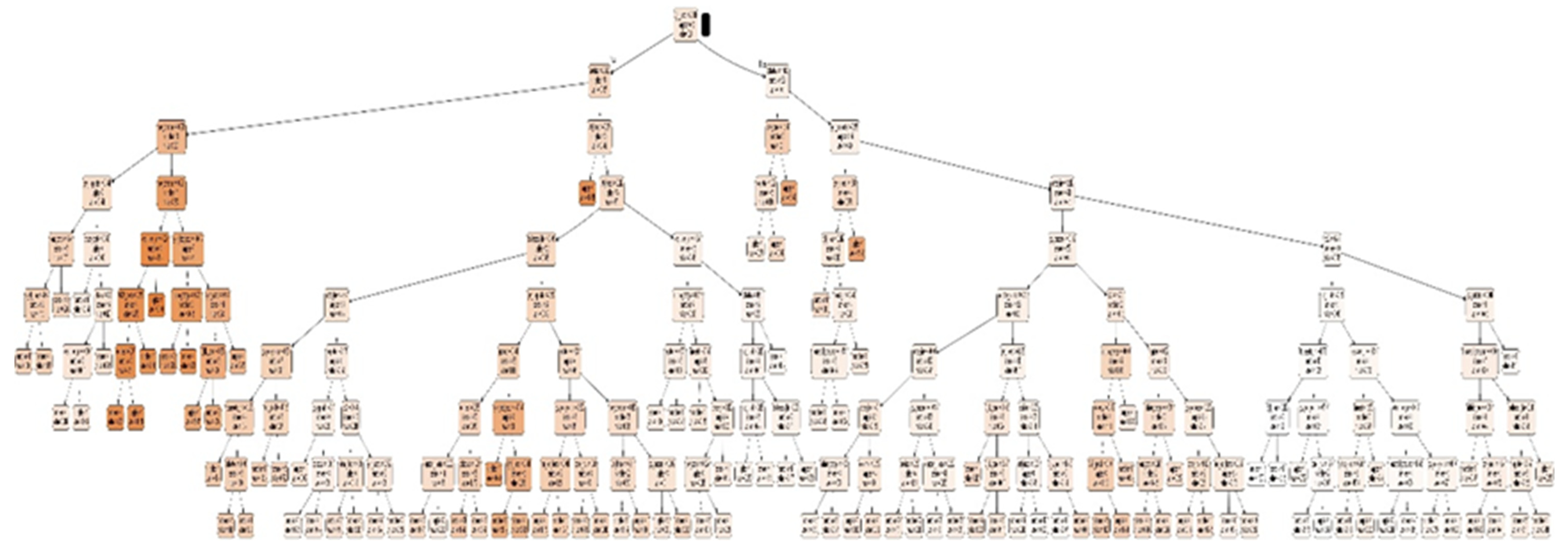
4.2. Machine-Enhanced Methods
4.3. Panel Data Analysis
5. Discussion
5.1. Property
5.2. Concentration in the Life and Non-Life Insurance Markets
5.3. Unit-Linked and Index-Linked Products
5.4. Size
5.5. Bond Markets
5.6. Government to Corporate Bonds
5.7. Private Debt
5.8. Collective Undertakings
5.9. Bonds and Equities
5.10. Household Disposable Income
5.11. Banking Concentration
5.12. Non-Performing Loans
5.13. CO2 Emissions
5.14. Interest Rates
6. Conclusions and Further Research
Author Contributions
Funding
Data Availability Statement
Conflicts of Interest
References
- Abdelzaher, Ahmed S., and Patricia Born. 2022. Formulating Policy for Bancassurance Activities Using Evidence from the US Financial Market. Journal of Insurance Issues 45: 1–27. [Google Scholar]
- Abduh, Muhamad, and Syaza Nawwarah Zein Isma. 2016. Dynamic financial model of life insurance and family takaful companies in Malaysia. Middle East Journal of Management 3: 72–93. [Google Scholar] [CrossRef]
- Abellán, Joaquín, and Andrés R. Masegosa. 2009. An Experimental Study about Simple Decision Trees for Bagging Ensemble on Datasets with Classification Noise. Berlin/Heidelberg: Springer, pp. 446–56. [Google Scholar] [CrossRef]
- Aldukhova, Evgeniya. V., Marina. V. Polyakova, and Konstantin. L. Polyakov. 2020. Institutional specifics of credit risk assessment for russian insurance companies. Journal of Institutional Studies 12: 101–21. [Google Scholar] [CrossRef]
- Ambrose, Jan M., and Anne M. Carroll. 1994. Using best’s ratings in life insurer insolvency prediction. Journal of Risk and Insurance 61: 317–27. [Google Scholar] [CrossRef]
- Athey, Susan, and Guido W. Imbens. 2019. Machine learning methods that economists should know about. Annual Review of Economics 11: 685–725. [Google Scholar] [CrossRef]
- Bailey, Delia, and Jonathan N. Katz. 2011. Implementing panel corrected standard errors in R: The pcse package. Journal of Statistical Software 42: 1–11. [Google Scholar] [CrossRef]
- Barboza, Flavio, Herbert Kimura, and Edward Altman. 2017. Machine learning models and bankruptcy prediction. Expert Systems with Applications 83: 405–17. [Google Scholar] [CrossRef]
- BarNiv, Ran, and Robert A. Hershbarger. 1990. Classifying financial distress in the life insurance industry. Journal of Risk and Insurance 57: 110–36. [Google Scholar] [CrossRef]
- Beck, Nathaniel, and Jonathan N. Katz. 1995. What to do (and not to do) with time-series cross-section data. American Political Science Review 89: 634–47. [Google Scholar] [CrossRef]
- Benali, Nadia, and Rochdi Feki. 2017. The impact of natural disasters on insurers’ profitability: Evidence from Property/Casualty Insurance company in United States. Research in International Business and Finance 42: 1394–400. [Google Scholar] [CrossRef]
- Berends, Kyal, Robert McMenamin, Thanases Plestis, and Richard J. Rosen. 2013. The sensitivity of life insurance firms to interest rate changes. Economic Perspectives 37: 47–78. [Google Scholar]
- Berrich, Olfa, Halim Dabbou, and Mohamed Imen Gallali. 2022. Over-the-counter market and corporate bond market development. International Journal of Entrepreneurship and Small Business 47: 284. [Google Scholar] [CrossRef]
- Berry, Michael J. A., and Gordon S. Linoff. 2009. Data Mining Techniques. Indianapolis: John Wiley & Sons. [Google Scholar]
- Bodie, Zvi, Alex Kane, and Alan J. Marcus. 2011. Investments and Portfolio Management, 9th ed. New York: McGrawn-Hill Irwin. [Google Scholar]
- Born, Patricia, and W. Kip Viscusi. 2006. The catastrophic effects of natural disasters on insurance markets. Journal of Risk and Uncertainty 33: 55–72. [Google Scholar] [CrossRef]
- Brockett, Patrick L., Linda L. Golden, Jaeho Jang, and Chuanhou Yang. 2006. A comparison of neural network, statistical methods, and variable choice for life insurers’ financial distress prediction. Journal of Risk and Insurance 73: 397–419. [Google Scholar] [CrossRef]
- Brockett, Patrick L., William W. Cooper, Linda L. Golden, and Utai Pitaktong. 1994. A neural network method for obtaining an early warning of insurer insolvency. Journal of Risk and Insurance 61: 402–24. [Google Scholar] [CrossRef]
- Brockett, Patrick L., William W. Cooper, Linda L. Golden, and Xiaohua Xia. 1997. A case study in applyingneural networks to predicting insolvency for property and casualty insurers. Journal of the Operational Research Society 48: 1153–62. [Google Scholar] [CrossRef]
- Browne, Mark J., and Robert E. Hoyt. 1995. Economic and market predictors of insolvencies in the property-liability insurance industry. Journal of Risk and Insurance 62: 309–27. [Google Scholar] [CrossRef]
- Bzdok, Danilo. 2017. Classical statistics and statistical learning in imaging neuroscience. Frontiers in Neuroscience 11: 273651. [Google Scholar] [CrossRef]
- Bzdok, Danilo, Martin Krzywinski, and Naomi Altman. 2017. Machine learning: A primer. Nature Methods 14: 1119. [Google Scholar] [CrossRef]
- Campbell, John Y., Jens Hilscher, and Jan Szilagyi. 2008. In search of distress risk. Journal of Finance 63: 2899–939. [Google Scholar] [CrossRef]
- Caporale, Guglielmo Maria, Mario Cerrato, and Xuan Zhang. 2017. Analysing the determinants of insolvency risk for general insurance firms in the UK. Journal of Banking & Finance 84: 107–22. [Google Scholar]
- Carmona, Pedro, Francisco Climent, and Alexandre Momparler. 2019. Predicting failure in the US banking sector: An extreme gradient boosting approach. International Review of Economics & Finance 61: 304–23. [Google Scholar]
- Chemmakha, Mohammed, Omar Habibi, and Mohamed Lazaar. 2022. Improving Machine Learning Models for Malware Detection Using Embedded Feature Selection Method. IFAC-PapersOnLine 55: 771–76. [Google Scholar] [CrossRef]
- Chen, James Ming. 2021. An introduction to machine learning for panel data. International Advances in Economic Research 27: 1–16. [Google Scholar] [CrossRef]
- Chen, Renbao, and Kie Ann Wong. 2004. The determinants of financial health of Asian insurance companies. Journal of Risk and Insurance 71: 469–99. [Google Scholar] [CrossRef]
- Chen, Xuanjuan, Zhenzhen Sun, Tong Yao, and Tong Yu. 2020. Does operating risk affect portfolio risk? Evidence from insurers’ securities holding. Journal of Corporate Finance 62: 101579. [Google Scholar] [CrossRef]
- Chen, Yueyun, Iskandar S. Hamwi, and Tim Hudson. 2001. The effect of ceded reinsurance on solvency of primary insurers. International Advances in Economic Research 7: 65–82. [Google Scholar] [CrossRef]
- Cheng, Jiang, and Mary A. Weiss. 2012. The Role of RBC, Hurricane Exposure, Bond Portfolio Duration, and Macroeconomic and Industry-wide Factors in Property–Liability Insolvency Prediction. Journal of Risk and Insurance 79: 723–50. [Google Scholar] [CrossRef]
- Chiet, Ng Shu, Saiful Hafizah Jaaman, Noriszura Ismail, and Siti Mariyam Shamsuddin. 2009. Insolvency prediction model using artificial neural network for Malaysian general insurers. Paper presented at the 2009 World Congress on Nature & Biologically Inspired Computing (NaBIC), Coimbatore, India, December 9–11; pp. 584–89. [Google Scholar]
- Chou, Pai-Lung, and Yu-Min Chang. 2011. The effect of the insurance company act on the capital benefit of investment in Taiwan’s life insurance industry. Journal of Statistics and Management Systems 14: 1041–55. [Google Scholar] [CrossRef]
- Climent, Francisco, Alexandre Momparler, and Pedro Carmona. 2019. Anticipating bank distress in the Eurozone: An extreme gradient boosting approach. Journal of Business Research 101: 885–96. [Google Scholar] [CrossRef]
- Cristina, Ciumaş, and Chiş Diana-Maria. 2015. Romanian Unit-linked Life Insurance Market. Procedia Economics and Finance 32: 1477–86. [Google Scholar] [CrossRef]
- Denuit, Michel, Donatien Hainaut, Julien Trufin, Michel Denuit, Donatien Hainaut, and Julien Trufin. 2020. Bagging Trees and Random Forests. Berlin/Heidelberg: Springer, pp. 107–30. [Google Scholar] [CrossRef]
- Dimitrov, Stanislav. 2022. Limitations of the framework to address value for money risk in the European unit-linked market. VUZF Review 7: 32. [Google Scholar] [CrossRef]
- Dissanayake, W. Dissanayake M. Bimba K., and P. S. N. Samarathunga. 2019. Factors Affecting for Loan Defaults with Special Reference to State Commercial Banks. Wayamba Journal of Management 10: 26–35. [Google Scholar] [CrossRef]
- Douglas, Graeme, Joseph Noss, and Nicholas Vause. 2017. The Impact of Solvency II Regulations on Life Insurers’ Investment Behaviour. Bank of England Working Paper No. 664. Available online: https://ssrn.com/abstract=2999604 (accessed on 7 July 2017).
- Doumpos, Michalis, Kostas Andriosopoulos, Emilios Galariotis, Georgia Makridou, and Constantin Zopounidis. 2017. Corporate failure prediction in the European energy sector: A multicriteria approach and the effect of country characteristics. European Journal of Operational Research 262: 347–60. [Google Scholar] [CrossRef]
- Drenovak, Mikica, Vladimir Ranković, Branko Urošević, and Ranko Jelic. 2020. Bond portfolio management under Solvency II regulation. The European Journal of Finance 27: 857–79. [Google Scholar] [CrossRef]
- du Jardin, Philippe. 2021. Forecasting corporate failure using ensemble of self-organizing neural networks. European Journal of Operational Research 288: 869–85. [Google Scholar] [CrossRef]
- Duijm, Patty, and Sophie Steins Bisschop. 2018. Short-termism of long-term investors? The investment behaviour of Dutch insurance companies and pension funds. Applied Economics 50: 3376–87. [Google Scholar] [CrossRef]
- Düll, Robert, Felix König, and Jana Ohls. 2017. On the exposure of insurance companies to sovereign risk—Portfolio investments and market forces. Journal of Financial Stability 31: 93–106. [Google Scholar] [CrossRef]
- EIOPA. 2015a. Delegated Regulation (EC) 2015/35. The European Insurance and Occupational Pensions Authority. Available online: https://eur-lex.europa.eu/eli/reg_del/2015/35/oj (accessed on 15 April 2022).
- EIOPA. 2015b. Guidelines on Own Risk and Solvency Assessment. The European Insurance and Occupational Pensions Authority. Available online: https://www.eiopa.europa.eu/publications/guidelines-own-risk-solvency-assessment-orsa_en (accessed on 15 April 2022).
- EIOPA. 2018. European Insurance Overview 2018. Available online: https://www.eiopa.europa.eu/publications/european-insurance-overview-2018_en (accessed on 15 October 2023).
- EIOPA. 2019. European Insurance Overview 2019. Available online: https://www.eiopa.europa.eu/publications/european-insurance-overview-2019_en (accessed on 15 October 2023).
- EIOPA. 2020. European Insurance Overview 2020. Available online: https://www.eiopa.europa.eu/publications/european-insurance-overview-2020_en (accessed on 15 October 2023).
- EIOPA. 2021. European Insurance Overview 2021. Available online: https://www.eiopa.europa.eu/publications/european-insurance-overview-2021_en (accessed on 15 October 2023).
- EIOPA. 2022a. EIOPA Publishes Application Guidance on How to Reflect Climate Change in ORSA. Available online: https://www.eiopa.europa.eu/eiopa-publishes-application-guidance-how-reflect-climate-change-orsa-2022-08-02_en (accessed on 14 August 2024).
- EIOPA. 2022b. European Insurance Overview 2022. Available online: https://www.eiopa.europa.eu/publications/european-insurance-overview-2022_en (accessed on 15 October 2023).
- EIOPA. 2023a. European Insurance Overview 2023. Available online: https://www.eiopa.europa.eu/publications/european-insurance-overview-report-2023_en (accessed on 15 October 2023).
- EIOPA. 2023b. Financial Stability Report December 2023. Available online: https://www.eiopa.europa.eu/publications/financial-stability-report-december-2023_en (accessed on 15 March 2024).
- Eling, Martin, and Ruo Jia. 2018. Business failure, efficiency, and volatility: Evidence from the European insurance industry. International Review of Financial Analysis 59: 58–76. [Google Scholar] [CrossRef]
- European Central Bank—ECB Data Portal. 2023. Available online: https://data.ecb.europa.eu/data/data-categories/financial-markets-and-interest-rates/securities-issues/csec-securities-issues-statistics/debt-securities (accessed on 15 October 2023).
- Fung, Derrick W. H., David Jou, Ai Ju Shao, and Jason J. H. Yeh. 2018. The implications of the China risk-oriented solvency system on the life insurance market. The Geneva Papers on Risk and Insurance-Issues and Practice 43: 615–32. [Google Scholar] [CrossRef]
- Gatzert, Nadine, and Dinah Heidinger. 2019. An Empirical Analysis of Market Reactions to the First Solvency and Financial Condition Reports in the European Insurance Industry. Journal of Risk and Insurance 87: 407–36. [Google Scholar] [CrossRef]
- Geng, Ruibin, Indranil Bose, and Xi Chen. 2015. Prediction of financial distress: An empirical study of listed Chinese companies using data mining. European Journal of Operational Research 241: 236–47. [Google Scholar] [CrossRef]
- Geurts, Pierre, Damien Ernst, and Louis Wehenkel. 2006. Extremely randomized trees. Machine Learning 63: 3–42. [Google Scholar] [CrossRef]
- Global Carbon Atlas. 2023. Available online: https://globalcarbonatlas.org/ (accessed on 15 March 2024).
- Graham, John, Mark T. Leary, and Michael R. Roberts. 2014. How Does Government Borrowing Affect Corporate Financing and Investment? No. w20581. Cambridge, MA: National Bureau of Economic Research. [Google Scholar]
- Guidara, Alaa, and Van Son Lai. 2015. Insurance Firms’ Capital Adjustment, Profitability, and Insolvency Risk Under Underwriting Cycles. Available online: https://ssrn.com/abstract=2675353 (accessed on 15 April 2022).
- Gupta, Anant. 2012. Unit linked insurance products (ULIPs)-Insurance or investment? Procedia-Social and Behavioral Sciences 37: 67–85. [Google Scholar] [CrossRef]
- Hada, Teodor, Nicoleta Bărbuță-Mișu, Iulia Cristina Iuga, and Dorin Wainberg. 2020. Macroeconomic determinants of nonperforming loans of Romanian banks. Sustainability 12: 7533. [Google Scholar] [CrossRef]
- Hao, Wenjing, Zhijian Qiu, and Lu Li. 2023. The investment and reinsurance game of insurers and reinsurers with default risk under CEV model. RAIRO-Operations Research 57: 2853–72. [Google Scholar] [CrossRef]
- Harrington, Scott E. 2005. Capital adequacy in insurance and reinsurance. Capital Adequacy beyond Basel: Banking, Securities, and Insurance 87: 88–89. [Google Scholar]
- Heaton, James B., Nick G. Polson, and Jan Hendrik Witte. 2017. Deep learning for finance: Deep portfolios. Applied Stochastic Models in Business and Industry 33: 3–12. [Google Scholar] [CrossRef]
- Heinrich, Michael, and Daniel Wurstbauer. 2014. Effects of Solvency II on Asset Allocation. No. eres2014_84. Bucharest: European Real Estate Society (ERES). Available online: https://ideas.repec.org/p/arz/wpaper/eres2014_84.html (accessed on 15 April 2022).
- Heinrich, Michael, and Daniel Wurstbauer. 2018. The impact of risk-based regulation on European insurers’ investment strategy. Zeitschrift für die gesamte Versicherungswissenschaft 107: 239–58. [Google Scholar] [CrossRef]
- Hoechle, Daniel. 2007. Robust standard errors for panel regressions with cross-sectional dependence. The Stata Journal 7: 281–312. [Google Scholar] [CrossRef]
- Höring, Dirk. 2013. Will Solvency II market risk requirements bite? The impact of Solvency II on insurers’ asset allocation. The Geneva Papers on Risk and Insurance-Issues and Practice 38: 250–73. [Google Scholar] [CrossRef]
- Hsu, Ker-Tah, and Tzung-Ming Yan. 2007. Applying grey models to categorical data-policyholder’s characteristics and purchase decision of unit linked insurance. Paper presented at the 2007 IEEE International Conference on Grey Systems and Intelligent Services, Nanjing, China, November 18–20; pp. 748–53. [Google Scholar]
- Insurance Europe and Oliver Wyman. 2013. Funding the Future Insurers’ Role as Institutional Investors. Available online: https://www.insuranceeurope.eu/publications/462/funding-the-future/ (accessed on 20 December 2023).
- Insurance Risk Data. 2023. Available online: https://www.insuranceriskdata.com/content/products/insurance-risk-database.html (accessed on 20 October 2023).
- International Monetary Fund. 2023a. Available online: https://www.imf.org/external/datamapper/profile/NGDP_RPCH@WEO/OEMDC/ADVEC/WEOWORLD (accessed on 20 October 2023).
- International Monetary Fund. 2023b. Financial Soundness Indicators. Available online: https://data.imf.org/?sk=51b096fa-2cd2-40c2-8d09-0699cc1764da (accessed on 20 October 2023).
- Jaśkiewicz, Dorota. 2020. Analysis of Capital Requirements in Life Insurance Sector Under Solvency II Regime: Evidence from Poland. Life Insurance in Europe: Risk Analysis and Market Challenges 50: 87–99. [Google Scholar]
- Joo, Bashir Ahmad. 2013. Analysis of Financial Stability of Indian Non Life Insurance Companies. Asian Journal of Finance & Accounting 5: 306. [Google Scholar]
- Jönsson, Kristian. 2005. Cross-sectional dependency and size distortion in a small-sample homogeneous panel data unit root test. Oxford Bulletin of Economics and Statistics 67: 369–92. [Google Scholar] [CrossRef]
- Jung, Hyunwoo, Young Dae Kwon, and Jin-Won Noh. 2022. Financial burden of catastrophic health expenditure on households with chronic diseases: Financial ratio analysis. BMC Health Services Research 22: 568. [Google Scholar] [CrossRef]
- Kartini, Endang. 2023. Financial Performance and the Effect on Sustainability Reports Disclosure, Company Size, and Solvency. KINERJA: Jurnal Manajemen Organisasi dan Industri 2: 21–30. [Google Scholar] [CrossRef]
- Kaur, Amarjeet, and Anand Bansal. 2016. Mis-selling of ULIPs-causes and regulatory approach towards unethical practices of mis-selling of ULIPs. International Journal of Indian Culture and Business Management 12: 141–54. [Google Scholar] [CrossRef]
- Kočović, Jelena, Blagoje Paunović, and Marija Jovović. 2015. Possibilities of creating optimal investment portfolio of insurance companies in Serbia. Ekonomika Preduzeća 63: 385–98. [Google Scholar] [CrossRef]
- Kouwenberg, Roy. 2018. Strategic asset allocation for insurers under Solvency II. Journal of Asset Management 19: 447–59. [Google Scholar] [CrossRef]
- Kramarić, Tomislava Pavić, Marko Miletić, and Renata Kožul Blaževski. 2019. Financial stability of insurance companies in selected CEE countries. Business Systems Research: International Journal of the Society for Advancing Innovation and Research in Economy 10: 163–78. [Google Scholar] [CrossRef]
- Krausch, Stefan. 2016. REITs as an Investment for German Insurance Companies. No. eres2016_314. Regensburg: European Real Estate Society (ERES). Available online: https://ideas.repec.org/p/arz/wpaper/eres2016_314.html (accessed on 15 April 2022).
- Krauss, Adam. 2024. The insurance implications of climate change. In Living with Climate Change. Amsterdam: Elsevier, pp. 295–341. [Google Scholar]
- Kudyba, Stephan, and Stephan Kudyba. 2014. Big Data, Mining, and Analytics. Boca Raton: Auerbach Publications. [Google Scholar]
- Kumar, P. Ravi, and Vadlamani Ravi. 2007. Bankruptcy prediction in banks and firms via statistical and intelligent techniques–A review. European Journal of Operational Research 180: 1–28. [Google Scholar] [CrossRef]
- Lee, Chen-Ying. 2018. The relationship between insurer solvency and reinsurance: Evidence from the Taiwan property-liability insurance industry. International Journal of Financial Services Management 9: 187–205. [Google Scholar] [CrossRef]
- Lee, Suk Hun, and Jorge L. Urrutia. 1996. Analysis and prediction of insolvency in the property-liability insurance industry: A comparison of logit and hazard models. Journal of Risk and Insurance 63: 121–30. [Google Scholar] [CrossRef]
- Leinonen, Jaakko. 2005. Indirect Real Estate Investments in the Finnish Private Pension Insurance Companies. No. eres2005_239. Dublin: European Real Estate Society (ERES). Available online: https://ideas.repec.org/p/arz/wpaper/eres2005_239.html (accessed on 15 April 2022).
- Lin, Weiwei, Ziming Wu, Longxin Lin, Angzhan Wen, and Jin Li. 2017. An ensemble random forest algorithm for insurance big data analysis. IEEE Access 5: 16568–75. [Google Scholar] [CrossRef]
- Martin, Daniel. 1977. Early warning of bank failure: A logit regression approach. Journal of Banking & Finance 1: 249–76. [Google Scholar]
- Mathur, Tanuj, and Ujjwal Kanti Paul. 2014. Performance appraisal of Indian non-life insurance companies: A DEA approach. Universal Journal of Management 2: 173–85. [Google Scholar] [CrossRef]
- Meyer, Paul A., and Howard W. Pifer. 1970. Prediction of bank failures. Journal of Finance 25: 853–68. [Google Scholar] [CrossRef]
- Moreno, Ignacio, Purificación Parrado-Martínez, and Antonio Trujillo-Ponce. 2020. Economic crisis and determinants of solvency in the insurance sector: New evidence from Spain. Accounting & Finance 60: 2965–94. [Google Scholar]
- Moundigbaye, Mantobaye, William S. Rea, and W. Robert Reed. 2018. Which panel data estimator should I use? A corrigendum and extension. Economics: The Open-Access, Open-Assessment E-Journal 12: 1–31. [Google Scholar] [CrossRef]
- Mselmi, Nada, Amine Lahiani, and Taher Hamza. 2017. Financial distress prediction: The case of French small and medium-sized firms. International Review of Financial Analysis 50: 67–80. [Google Scholar] [CrossRef]
- Muteru, Milka W., and Job Omagwa. 2024. Macroeconomic Dynamics and Profitability of Insurance Firms Listed at Nairobi Securities Exchange, Kenya. Journal of Finance and Accounting 8: 132–48. [Google Scholar] [CrossRef]
- Müller, Andreas C., and Sarah Guido. 2017. Introduction to Machine Learning with Python: A Guide for Data Scientists. Sebastopol: O’Reilly Media, Inc., pp. 17–18, 78. [Google Scholar]
- Nadalizadeh, Ameneh, Kambiz Kiani, Shamseddin Hoseini, and Kambiz Peykarjou. 2019. The Impact of Oil Price Movements on Bank Nonperforming Loans (NPLs): The Case of Iran. Petroleum Business Review 3: 63–78. [Google Scholar]
- Newman, Thomas B., and Warren S. Browner. 1991. In defense of standardized regression coefficients. Epidemiology 2: 383–86. [Google Scholar] [CrossRef] [PubMed]
- Niedrig, Tobias, and Helmut Gründl. 2015. The effects of contingent convertible (CoCo) bonds on insurers’ capital requirements under Solvency II. The Geneva Papers on Risk and Insurance-Issues and Practice 40: 416–43. [Google Scholar] [CrossRef]
- Nneka, Uguanyi Jacinta, Chi Aloysius Ngong, Okeke Augustina Ugoada, and Josaphat Uchechukwu Joe Onwumere. 2022. Effect of bond market development on economic growth of selected developing countries. Journal of Economic and Administrative Sciences. [Google Scholar] [CrossRef]
- OECD. 2011. Household disposable income. In OECD Factbook 2011–12: Economic, Environmental and Social Statistics. Paris: OECD Publishing. [Google Scholar] [CrossRef]
- OECD. 2012. The private debt market and capital market regulation. In Capital Markets in the Dominican Republic: Tapping the Potential for Development. Paris: OECD Publishing. [Google Scholar] [CrossRef]
- OECD. 2023. Data Base. Available online: https://www.oecd.org/en/data/indicators/long-term-interest-rates.html (accessed on 20 October 2023).
- Ozili, Peterson K., Asma Salman, and Qaisar Ali. 2020. The impact of foreign direct investment inflows on nonperforming loans: The case of UAE. Available online: https://ssrn.com/abstract=3742785 (accessed on 15 October 2023). [CrossRef]
- Papadopoulos, Sokratis, Elie Azar, Wei-Lee Woon, and Constantine E. Kontokosta. 2017. Evaluation of tree-based ensemble learning algorithms for building energy performance estimation. Journal of Building Performance Simulation 11: 322–32. [Google Scholar] [CrossRef]
- Park, Sojung Carol, and Xiaoying Xie. 2014. Reinsurance and systemic risk: The impact of reinsurer downgrading on property–casualty insurers. Journal of Risk and Insurance 81: 587–622. [Google Scholar] [CrossRef]
- Pasiouras, Fotios, and Chrysovalantis Gaganis. 2013. Regulations and soundness of insurance firms: International evidence. Journal of Business Research 66: 632–42. [Google Scholar] [CrossRef]
- Peters, B. Guy. 2018. The Politics of Bureaucracy: An Introduction to Comparative Public Administration. London: Routledge. [Google Scholar]
- Pottier, Steven W. 2007. The determinants of private debt holdings: Evidence from the life insurance industry. Journal of Risk and Insurance 74: 591–612. [Google Scholar] [CrossRef]
- Rauch, Jannes, and Sabine Wende. 2015. Solvency prediction for property-liability insurance companies: Evidence from the financial crisis. Geneva Papers on Risk and Insurance-Issues and Practice 40: 47–65. [Google Scholar] [CrossRef]
- Ritho, Bonface Mugo. 2023. The Impact of Loss Ratio on the Financial Stability of Insurance Firms in Kenya. Journal of Finance and Accounting 7: 22–41. [Google Scholar] [CrossRef]
- Rustam, Zuherman, and Frederica Yaurita. 2018. Insolvency prediction in insurance companies using support vector machines and fuzzy kernel c-means. Journal of Physics: Conference Series 1028: 012118. [Google Scholar] [CrossRef]
- Rustam, Zuherman, and G. Saragih. 2021. Prediction insolvency of insurance companies using random forest. Journal of Physics: Conference Series 1752: 012036. [Google Scholar] [CrossRef]
- Safari, A., N. Sarlak, and R. Nasiri. 2015. Relationship between Solvency and Financial Ratios in Iranian Insurance Institutions. Cumhuriyet Science Journal 36: 2807–17. [Google Scholar]
- Sarker, Iqbal H. 2021. Machine learning: Algorithms, real-world applications and research directions. SN Computer Science 2: 160. [Google Scholar] [CrossRef]
- Sharpe, Ian G., and Andrei Stadnik. 2007. Financial distress in Australian general insurers. Journal of Risk and Insurance 74: 377–99. [Google Scholar] [CrossRef]
- Sharpe, William F. 1992. Asset allocation: Management style and performance measurement. Journal of portfolio Management 18: 7–19. [Google Scholar] [CrossRef]
- Sheehan, Barry, Martin Mullins, Darren Shannon, and Orla McCullagh. 2023. On the benefits of insurance and disaster risk management integration for improved climate-related natural catastrophe resilience. Environment Systems and Decisions 43: 639–48. [Google Scholar] [CrossRef]
- Shim, Jeungbo. 2017. An investigation of market concentration and financial stability in property–liability insurance industry. Journal of Risk and Insurance 84: 567–97. [Google Scholar]
- Shiu, Yung-Ming. 2005. The determinants of solvency in the United Kingdom life insurance market. Applied Economics Letters 12: 339–44. [Google Scholar] [CrossRef]
- Siddik, Md Nur Alam, Md Emran Hosen, Md Firoze Miah, Sajal Kabiraj, Shanmugan Joghee, and Swamynathan Ramakrishnan. 2022. Impacts of insurers’ financial insolvency on non-life insurance companies’ profitability: Evidence from Bangladesh. International Journal of Financial Studies 10: 80. [Google Scholar] [CrossRef]
- Sinkey, Joseph F., Jr. 1975. A multivariate statistical analysis of the characteristics of problem banks. Journal of Finance 30: 21–36. [Google Scholar] [CrossRef]
- Siopi, Evaggelia, Thomas Poufinas, James Ming Chen, and Charalampos Agiropoulos. 2023. Can Regulation Affect the Solvency of Insurers? New Evidence from European Insurers. International Advances in Economic Research 29: 15–30. [Google Scholar] [CrossRef]
- Solomon, Susan, Gian-Kasper Plattner, Reto Knutti, and Pierre Friedlingstein. 2009. Irreversible climate change due to carbon dioxide emissions. Proceedings of the National Academy of Sciences 106: 1704–9. [Google Scholar] [CrossRef]
- Stack Overflow. 2024. Converting Dot to png in Python. Available online: https://stackoverflow.com/questions/5316206/converting-dot-to-png-in-python (accessed on 22 January 2024).
- Sutanto, Shelby, Iwan Lesmana, Meco Sitardja, and Dheny Biantara. 2023. The Impact of Claim Expenses, Underwriting Risk, Profitability, Company Size and Retention Ratio on Solvency of Insurance Industry. Indonesian Journal of Accounting and Governance 7: 84–96. [Google Scholar] [CrossRef]
- Svensson, Lars E. O. 2021. Household Debt Overhang Did Hardly Cause a Larger Spending Fall during the Financial Crisis in Australia. Cambridge, MA: National Bureau of Economic Research. [Google Scholar] [CrossRef]
- Szaniewski, Daniel. 2021. Investment activities of polish insurance companies before and after Solvency II. Foundations of Management 13: 229–42. [Google Scholar] [CrossRef]
- Tam, Kar Yan, and Melody Y. Kiang. 1992. Managerial applications of neural networks: The case of bank failure predictions. Management Science 38: 926–47. [Google Scholar] [CrossRef]
- Tanaka, Katsuyuki, Takuji Kinkyo, and Shigeyuki Hamori. 2016. Random forests-based early warning system for bank failures. Economics Letters 148: 118–21. [Google Scholar] [CrossRef]
- Tian, Shaonan, Yan Yu, and Hui Guo. 2015. Variable selection and corporate bankruptcy forecasts. Journal of Banking & Finance 52: 89–100. [Google Scholar]
- Topol, Eric. 2019. Deep Medicine: How Artificial Intelligence Can Make Healthcare Human Again. Paris: Hachette UK. [Google Scholar]
- Trieschmann, James S., and George E. Pinches. 1973. A multivariate model for predicting financially distressed PL insurers. Journal of Risk and Insurance 40: 327–38. [Google Scholar] [CrossRef]
- Tsvetkova, Lyudmila. 2023. Dynamic Maintenance of Solvency of the Russian Insurance Companies: The Evidence from Russian Insurers. Кoрпoративные финансы 17: 85–94. [Google Scholar] [CrossRef]
- Ugbam, Charles Ogechukwu, Chi Aloysius Ngong, Ishaku Prince Abner, and Godwin Imo Ibe. 2023. Bond market development and economic growth nexus in developing countries: A GMM approach. Journal of Economic and Administrative Sciences. [Google Scholar] [CrossRef]
- Vargas, María Jesús Segovia, José Antonio Gil Fana, Antonio José Heras Martínez, José Luis Vilar Zanón, and Alicia Sanchis Arellano. 2003. Using Rough Sets to Predict Insolvency of Spanish Non-Life Insurance Companies. No. 03-02. Madrid: Universidad Complutense de Madrid, Facultad de Ciencias Económicas y Empresariales. [Google Scholar]
- Vojvodić, Miljković Nevenka M., Milica S. Cvetković, and Marija M. Lukić. 2023. Impact of unit-linked insurance on development of the insurance market and the financial market in the Republic of Serbia. Tokovi Osiguranja 39: 538–89. [Google Scholar] [CrossRef]
- Wang, Alan T. 2017. NPLs, Moral Hazards, and Bond Markets. Available online: https://ssrn.com/abstract=2961139 (accessed on 20 October 2023).
- Wang, Gang, Jian Ma, and Shanlin Yang. 2014. An improved boosting based on feature selection for corporate bankruptcy prediction. Expert Systems with Applications 41: 2353–61. [Google Scholar] [CrossRef]
- Witkowska, Justyna. 2023. The Life And Non-Life Insurance Market In The European Union. Olsztyn Economic Journal 18: 157–70. [Google Scholar] [CrossRef]
- Wolpert, David H. 1996. The lack of a priori distinctions between learning algorithms. Neural Computation 8: 1341–90. [Google Scholar] [CrossRef]
- Wolski, Rafal, and Magdalena Zaleczna. 2010. The Real Estate Investment Of Insurance Companies In Polish Conditions. No. eres2010_264. Milan: European Real Estate Society (ERES). [Google Scholar]
- Wolski, Rafal, and Magdalena Zaleczna. 2011. The real estate investment of insurance companies in Poland. Journal of Property Investment & Finance 29: 74–82. [Google Scholar]
- World Bank Open Data. 2023. Available online: https://data.worldbank.org/?cid=ECR_GA_worldbank_EN_EXTP_search&s_kwcid=AL!18468!3!704632427243!b!!g!!world%20bank%20projects&gad_source=1 (accessed on 20 October 2023).
- Wünsch, Pavel. 2019. Solvency Position of Insurers on Czech Market at Day-One Reporting. Berlin/Heidelberg: Springer, pp. 279–87. [Google Scholar] [CrossRef]
- Yang, Qining. 2023. Research on the Impact of Climate Change on Insurance Companies. Advances in Economics, Management and Political Sciences 9: 264–69. [Google Scholar] [CrossRef]
- Zariņa, Ilze, Irina Voronova, and Gaida Pettere. 2018. Assessment of the stability of insurance companies: The case of Baltic non-life insurance market. Economics and Business 32: 102–11. [Google Scholar] [CrossRef]
- Zhang, Le, Ye Ren, and Ponnuthurai N. Suganthan. 2014. Towards generating random forests via extremely randomized trees. institute of electrical electronics engineers. Paper presented at the 2014 International Joint Conference on Neural Networks (IJCNN), Beijing, China, July 6–11. [Google Scholar]
- Zhang, Li, and Norma Nielson. 2015. Solvency Analysis and Prediction in Property–Casualty Insurance: Incorporating Economic and Market Predictors. Journal of Risk and Insurance 82: 97–124. [Google Scholar] [CrossRef]
- Ziemele, Jana, and Irina Voronova. 2013. Financial stability of the EU’s insurance companies. Economics and Management 18: 436–48. [Google Scholar] [CrossRef]


| Variables | Description | Role | Source |
|---|---|---|---|
| Target variable | |||
| SCR ratio | Solvency Capital Requirement ratio. | Solvency of the insurer | Insurance Risk Data (2023) |
| Features (Explanatory Variables) | |||
| Size | Total assets (natural logarithm). | Size of the insurance group | Insurance Risk Data (2023) |
| Property | Property as percent of investments. | Investment portfolio diversification | Insurance Risk Data (2023) |
| Government bonds to corporate bonds | Ratio of investments in government bonds to investments in corporate bonds. | Diversification of the insurance group’s bond investment portfolio | Insurance Risk Data (2023) |
| Collective | Collective investment undertakings as percent of investments. | Investment portfolio diversification | Insurance Risk Data (2023) |
| Unit_linked | Unit_linked and Index_linked as percent of liabilities. | Risk transfer from insurer to policyholder | Insurance Risk Data (2023) |
| Equities | Equities as percent of total investments. | Investment portfolio diversification | Insurance Risk Data (2023) |
| Bonds | Bonds as percent of total investments. | Investment portfolio diversification | Insurance Risk Data (2023) |
| Life concentration | Market share of the 3 biggest life premium writers of the national gross written premium. | Competition in the life insurance sector | EIOPA (2018, 2019, 2020, 2021, 2022b, 2023a) |
| Non-life concentration | Market share of the 3 biggest non-life premium writers of the national gross written premium. | Competition in the non-life insurance sector | EIOPA (2018, 2019, 2020, 2021, 2022b, 2023a) |
| Bond market | It covers long-term bonds and notes, treasury bills, commercial paper, and other short-term notes issued on domestic markets. | Domestic bond market development | European Central Bank—ECB Data Portal (2023) |
| Private debt | Total stock of loans and debt securities issued by households and nonfinancial corporations as a share of GDP. | Domestic private dept development | International Monetary Fund (2023b) |
| Real GDP growth | The real economic growth rate, or real GDP growth rate, measures economic growth, as expressed by the gross domestic product (GDP), from one period to another, adjusted for inflation or deflation. | Economic growth | World Economic Outlook (October 2023), International Monetary Fund (2023a) |
| Interest | Long-term interest rates are determined by the lender’s price, the borrower’s risk, and the decline in the capital value of government bonds maturing in ten years. | Low interest rates encourage investment in new equipment, while high interest rates discourage it, contributing to economic growth | OECD (2023) |
| Household spending | Household consumption expenditure is the final consumption expenditure made by residents to meet their daily needs, including housing, water, electricity, gas, and other fuels. | Household living costs | World Bank Open Data (2023) |
| Inflation change | Inflation rate, average consumer prices (annual percent change). | The rise in the cost of living in a country | World Bank Open Data (2023) |
| Government expenditure | General government expenditure indicates the size of government in each country as share of GDP, its approaches to public goods and services provision, and social protection measures. | Government spending in relation to GDP refers to public goods and services and social protection | International Monetary Fund (2023a) |
| Banking concentration | Banking concentration: percent of bank assets held by the top three banks. | Controlling for alternative choices in the cash deposits of insurance groups | International Monetary Fund (2023a) |
| Regulatory capital | Regulatory capital to risk-weighted assets. The capital adequacy of deposit-taking institutions. | The degree of robustness of financial institutions | International Monetary Fund (2023b) |
| Non-performing loans | The ratio of non-performing loans to total gross loans, as instability can disrupt economic activity and impose costs. A high ratio indicates loan portfolio deterioration. | Financial system strength | International Monetary Fund (2023b) |
| CO2 emissions | CO2 emissions per person are measured as the total CO2 produced by a country as a result of human activities divided by the population of that country. Carbon dioxide emissions are the main cause of global climate change, but the allocation of responsibility among regions, countries, and individuals remains a contentious issue in international discussions. | Climate change | Global Carbon Atlas (2023) |
| Mean | Standard Deviation | Min | Max | 5th Percentile | 10th Percentile | 25th Percentile | 75th Percentile | 90th Percentile | 95th Percentile | |
|---|---|---|---|---|---|---|---|---|---|---|
| Size | 17.198 | 1.651 | 3.807 | 20.566 | 14.973 | 15.273 | 16.143 | 18.309 | 19.279 | 19.964 |
| Property | 0.047 | 0.048 | 0.000 | 0.275 | 0.000 | 0.001 | 0.009 | 0.066 | 0.109 | 0.152 |
| Government bonds to corporate bonds | 2.022 | 5.402 | 0.000 | 82.399 | 0.096 | 0.254 | 0.468 | 1.733 | 3.261 | 5.927 |
| Collective | 0.172 | 0.152 | 0.000 | 0.757 | 0.010 | 0.019 | 0.048 | 0.253 | 0.402 | 0.462 |
| Unit_linked | 0.201 | 0.236 | −0.552 | 2.865 | 0.003 | 0.008 | 0.037 | 0.289 | 0.512 | 0.677 |
| Equities | 0.040 | 0.061 | 0.000 | 0.466 | 0.000 | 0.001 | 0.008 | 0.051 | 0.085 | 0.121 |
| Bonds | 0.653 | 0.173 | 0.141 | 0.993 | 0.322 | 0.395 | 0.547 | 0.787 | 0.852 | 0.896 |
| Life concentration | 0.380 | 0.133 | 0.240 | 0.781 | 0.242 | 0.243 | 0.270 | 0.450 | 0.600 | 0.640 |
| Non-life concentration | 0.362 | 0.145 | 0.140 | 0.700 | 0.140 | 0.149 | 0.260 | 0.466 | 0.58 | 0.6 |
| Bond market | 0.682 | 0.291 | 0.111 | 1.411 | 0.246 | 0.338 | 0.470 | 0.916 | 1.105 | 1.187 |
| Private debt | 1.664 | 0.554 | 0.670 | 4.068 | 1.103 | 1.175 | 1.222 | 2.116 | 2.419 | 2.497 |
| Real GDP growth | 0.015 | 0.035 | −0.112 | 0.131 | −0.065 | −0.038 | 0.011 | 0.029 | 0.048 | 0.064 |
| Interest | 0.006 | 0.009 | −0.005 | 0.061 | −0.004 | −0.004 | 0.000 | 0.011 | 0.017 | 0.022 |
| Household spending | 0.524 | 0.056 | 0.302 | 0.650 | 0.437 | 0.449 | 0.503 | 0.540 | 0.601 | 0.629 |
| Inflation change | 0.023 | 0.024 | −0.011 | 0.144 | 0.001 | 0.002 | 0.008 | 0.025 | 0.069 | 0.082 |
| Government expenditure | 0.217 | 0.022 | 0.157 | 0.264 | 0.186 | 0.189 | 0.198 | 0.236 | 0.246 | 0.255 |
| Banking concentration | 0.696 | 0.121 | 0.332 | 0.959 | 0.450 | 0.579 | 0.634 | 0.791 | 0.876 | 0.905 |
| Regulatory capital | 0.195 | 0.021 | 0.138 | 0.269 | 0.167 | 0.177 | 0.180 | 0.206 | 0.224 | 0.233 |
| Non-performing loans | 0.028 | 0.023 | 0.003 | 0.171 | 0.009 | 0.010 | 0.020 | 0.029 | 0.035 | 0.060 |
| CO2 emissions | 14.214 | 3.158 | 6.870 | 29.701 | 9.311 | 10.010 | 11.748 | 16.179 | 17.816 | 18.660 |
| SCR ratio | 2.547 | 1.135 | 1.000 | 8.560 | 1.437 | 1.564 | 1.890 | 2.885 | 3.836 | 4.692 |
| Size | Property | Government Bonds to Corporate Bonds | COLLECTIVE | Unit_Linked | Equities | Bonds | Life Concentration | Non-Life Concentration | Bond Market | Private Debt | Real GDP Growth | Interest | Household Spending | Inflation Change | Government Expenditure | Banking Concentration | Regulatory Capital | Non-Performing Loans | Co2 Emissions | SCR Ratio | |
|---|---|---|---|---|---|---|---|---|---|---|---|---|---|---|---|---|---|---|---|---|---|
| Size | 1 | ||||||||||||||||||||
| Property | −0.2656 | 1 | |||||||||||||||||||
| Gov_bonds to corp_bonds | −0.1766 | −0.0187 | 1 | ||||||||||||||||||
| Collective | −0.0898 | −0.0198 | −0.1782 | 1 | |||||||||||||||||
| Unit_linked | 0.1524 | −0.0225 | −0.1204 | −0.2197 | 1 | ||||||||||||||||
| Equities | −0.0240 | 0.3316 | −0.0407 | −0.2205 | 0.1240 | 1 | |||||||||||||||
| Bonds | 0.0171 | −0.2520 | 0.1353 | −0.6131 | −0.1202 | −0.2227 | 1 | ||||||||||||||
| Life concentration | −0.2024 | 0.3905 | 0.0968 | −0.2269 | 0.2527 | 0.1672 | −0.0074 | 1 | |||||||||||||
| Non-life concentration | −0.2246 | 0.2248 | 0.1654 | −0.2123 | 0.4620 | 0.1770 | −0.1342 | 0.6441 | 1 | ||||||||||||
| Bond market | 0.1544 | −0.0580 | 0.0818 | −0.2633 | −0.1090 | 0.0210 | 0.2827 | −0.0513 | −0.1562 | 1 | |||||||||||
| Private debt | 0.2082 | 0.1188 | −0.1420 | −0.2272 | 0.4434 | 0.3480 | −0.0336 | 0.2632 | 0.0564 | −0.1247 | 1 | ||||||||||
| Real GDP growth | −0.0552 | 0.0380 | 0.0329 | −0.0558 | 0.0702 | 0.0601 | −0.0266 | 0.0783 | 0.0817 | −0.1349 | −0.0161 | 1 | |||||||||
| Interest | −0.0704 | 0.0753 | 0.3206 | −0.2458 | 0.0933 | 0.0279 | 0.1216 | 0.2280 | 0.3178 | 0.2868 | −0.1140 | 0.2503 | 1 | ||||||||
| Household spending | 0.0375 | −0.1116 | 0.1873 | −0.1452 | −0.1945 | −0.0274 | 0.1433 | −0.1052 | −0.0482 | 0.7600 | −0.5178 | −0.0323 | 0.3803 | 1 | |||||||
| Inflation change | −0.0029 | 0.0644 | −0.0501 | 0.0823 | 0.1238 | −0.0100 | −0.1565 | 0.0600 | 0.1130 | −0.0215 | −0.0288 | 0.3517 | 0.5364 | −0.0553 | 1 | ||||||
| Government expenditure | 0.2115 | 0.0899 | −0.1260 | −0.0185 | 0.2124 | 0.2529 | −0.1757 | 0.1501 | −0.0558 | −0.1593 | 0.6323 | −0.1128 | −0.2808 | −0.4391 | 0.0477 | 1 | |||||
| Banking concentration | −0.0171 | 0.0984 | −0.1337 | 0.2553 | 0.0276 | 0.0112 | −0.2701 | 0.0954 | 0.0835 | −0.6425 | 0.1575 | −0.0121 | −0.3059 | −0.5954 | 0.0057 | 0.5535 | 1 | ||||
| Regulatory capital | 0.0901 | 0.1293 | −0.0454 | −0.0387 | 0.5594 | 0.2967 | −0.3436 | 0.3175 | 0.5174 | −0.3411 | 0.5561 | 0.0138 | −0.0716 | −0.4682 | 0.1596 | 0.4875 | 0.2887 | 1 | |||
| Non-performing loans | −0.1269 | −0.0598 | 0.4967 | −0.1484 | −0.2996 | −0.1706 | 0.3111 | −0.0856 | −0.0196 | 0.2737 | −0.3423 | −0.0099 | 0.2903 | 0.3387 | −0.2339 | −0.3467 | −0.1686 | −0.5344 | 1 | ||
| CO2 emissions | −0.2168 | −0.1164 | 0.1510 | 0.1329 | −0.3995 | −0.2956 | 0.0593 | −0.0390 | −0.0447 | −0.2413 | −0.5299 | 0.0856 | −0.0013 | 0.0284 | −0.0481 | −0.4550 | −0.0094 | −0.3459 | 0.1845 | 1 | |
| SCR ratio | −0.0264 | −0.0152 | −0.0871 | 0.2752 | −0.2983 | −0.1557 | −0.1170 | −0.4238 | −0.2723 | −0.2832 | −0.2968 | 0.0000 | −0.2338 | −0.1305 | −0.0124 | −0.1564 | 0.1325 | −0.1771 | −0.0062 | 0.2742 | 1 |
| R2 | RMSE | |
|---|---|---|
| Training set score: | 0.386375 | 0.783342 |
| Test set score: | 0.338236 | 0.745446 |
| Variables | Coefficients | p-values |
| Size | 0.02969 | 0.66016 |
| Property | 0.136532 ** | 0.00495 |
| Government bonds to corporate bonds | −0.03930 | 0.45367 |
| Collective | −0.04763 | 0.45970 |
| Unit_linked | −0.227071 *** | 0.00021 |
| Equities | −0.08617 | 0.08162 |
| Bonds | −0.07999 | 0.22194 |
| Life concentration | −0.414205 *** | 0.00000 |
| Non-life concentration | 0.10211 | 0.24075 |
| Bond market | −0.303901 *** | 0.00083 |
| Private debt | −0.06004 | 0.52401 |
| Real GDP growth | 0.00570 | 0.89916 |
| Interest | −0.158275 * | 0.03175 |
| Household spending | 0.00830 | 0.94519 |
| Inflation change | 0.07852 | 0.22976 |
| Government expenditure | −0.04218 | 0.59264 |
| Banking concentration | −0.06013 | 0.41616 |
| Regulatory capital | −0.02360 | 0.79039 |
| Non-performing loans | −0.00628 | 0.92353 |
| CO2 emissions | 0.06236 | 0.27160 |
| Intercept | 0.000000 | 1.00000 |
| R2 | RMSE | |||
|---|---|---|---|---|
| Train | Test | Train | Test | |
| Linear regression | 0.386375 | 0.338101 | 0.783342 | 0.745522 |
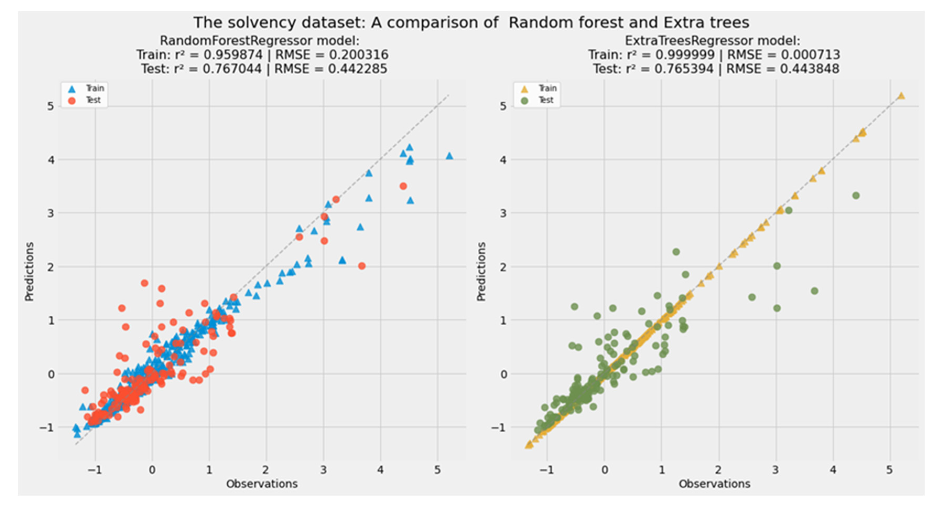
| Random forest regression | 0.959874 | 0.767044 | 0.200316 | 0.442285 |
| Extra trees regression | 0.999999 | 0.765394 | 0.000713 | 0.443848 |
| Gradient boosting regression | 0.799700 | 0.628627 | 0.447549 | 0.558431 |
| XGBoost (extreme gradient boosting regression) | 0.917349 | 0.655580 | 0.287491 | 0.537785 |
| SVM (support vector machine) | 0.628154 | 0.496709 | 0.609792 | 0.650091 |
| MLP Regression (Multi-Level Perceptron regression) | 0.838898 | 0.570523 | 0.400128 | 0.600530 |
| No of Observations | 462 | 154 | 462 | 154 |
| R2 | RMSE | ||
|---|---|---|---|
| Train | 0.999999 | 0.000713 | |
| Test | 0.765394 | 0.443848 | |
| Dependent Variable: SCR ratio | |||
| Variable: | Importance: | Variable: | Importance: |
| Property | 0.21 | Bonds | 0.03 |
| Life concentration | 0.18 | Household spending | 0.01 |
| Unit_linked | 0.16 | Banking concentration | 0.01 |
| Size | 0.1 | Non-performing loans | 0.01 |
| Bond market | 0.07 | CO2 emissions | 0.01 |
| Non-Life concentration | 0.06 | Real GDP growth | 0 |
| Government bonds to corporate bonds | 0.05 | Interest | 0 |
| Private debt | 0.04 | Inflation change | 0 |
| Collective | 0.03 | Government expenditure | 0 |
| Equities | 0.03 | Regulatory capital | 0 |
| Train | Test | ||
| No. of Observations | 462 | 154 | |
| Dependent Variable: SCR Ratio | ||||||
|---|---|---|---|---|---|---|
| Variable | Coef. | St. Err. | t-Value | p-Value | 95% Confidence | Interval |
| Size | −0.026 | 0.032 | −0.81 | 0.419 | −0.089 | 0.037 |
| Property | 2.353 ** | 0.921 | 2.56 | 0.011 | 0.548 | 4.157 |
| Government bonds to corporate bonds | −0.007 ** | 0.003 | −2.26 | 0.024 | −0.013 | −0.001 |
| Collective | 0.452 | 0.363 | 1.25 | 0.212 | −0.258 | 1.163 |
| Unit_linked | −0.372 | 0.345 | −1.08 | 0.282 | −1.049 | 0.305 |
| Equities | −0.519 | 0.767 | −0.68 | 0.499 | −2.023 | 0.986 |
| Bonds | −0.296 | 0.275 | −1.08 | 0.282 | −0.834 | 0.243 |
| Life concentration | −2.972 ** | 0.546 | −5.44 | 0 | −4.043 | −1.901 |
| Non-Life concentration | −0.039 | 0.606 | −0.06 | 0.948 | −1.227 | 1.148 |
| Bond market | −0.854 ** | 0.256 | −3.33 | 0.001 | −1.356 | −0.352 |
| Private debt | −0.415 ** | 0.113 | −3.69 | 0 | −0.636 | −0.194 |
| Real GDP growth | 0.139 | 0.422 | 0.33 | 0.741 | −0.687 | 0.966 |
| Interest | −4.573 | 6.166 | −0.74 | 0.458 | −16.659 | 7.513 |
| Household spending | −2.56 * | 1.005 | −2.55 | 0.011 | −4.531 | −0.59 |
| Inflation change | 0.849 | 1.682 | 0.5 | 0.614 | −2.449 | 4.146 |
| Government expenditure | 2.931 | 2.956 | 0.99 | 0.321 | −2.862 | 8.724 |
| Banking concentration | −0.871 | 0.585 | −1.49 | 0.137 | −2.018 | 0.276 |
| Regulatory capital | −1.913 | 2.37 | −0.81 | 0.419 | −6.558 | 2.731 |
| Non-performing loans | −0.514 | 1.538 | −0.33 | 0.738 | −3.528 | 2.5 |
| CO2 emissions | 0.039 * | 0.018 | 2.13 | 0.034 | 0.003 | 0.075 |
| Constant | 6.681 ** | 0.918 | 7.28 | 0 | 4.882 | 8.481 |
| Mean dependent var | 2.547 | Standard dependent var | 1.135 | |||
| R-squared | 0.454 | No. of observations | 616 | |||
| Chi-square | 433.169 | Prob > chi2 | 0 | |||
Disclaimer/Publisher’s Note: The statements, opinions and data contained in all publications are solely those of the individual author(s) and contributor(s) and not of MDPI and/or the editor(s). MDPI and/or the editor(s) disclaim responsibility for any injury to people or property resulting from any ideas, methods, instructions or products referred to in the content. |
© 2024 by the authors. Licensee MDPI, Basel, Switzerland. This article is an open access article distributed under the terms and conditions of the Creative Commons Attribution (CC BY) license (https://creativecommons.org/licenses/by/4.0/).
Share and Cite
Poufinas, T.; Siopi, E. Investment Portfolio Allocation and Insurance Solvency: New Evidence from Insurance Groups in the Era of Solvency II. Risks 2024, 12, 191. https://doi.org/10.3390/risks12120191
Poufinas T, Siopi E. Investment Portfolio Allocation and Insurance Solvency: New Evidence from Insurance Groups in the Era of Solvency II. Risks. 2024; 12(12):191. https://doi.org/10.3390/risks12120191
Chicago/Turabian StylePoufinas, Thomas, and Evangelia Siopi. 2024. "Investment Portfolio Allocation and Insurance Solvency: New Evidence from Insurance Groups in the Era of Solvency II" Risks 12, no. 12: 191. https://doi.org/10.3390/risks12120191
APA StylePoufinas, T., & Siopi, E. (2024). Investment Portfolio Allocation and Insurance Solvency: New Evidence from Insurance Groups in the Era of Solvency II. Risks, 12(12), 191. https://doi.org/10.3390/risks12120191