Article

Estimating the Acceptance Probabilities of Consumer Loan Offers in an Online Loan Comparison and Brokerage Platform

by
Renatas Špicas
*,
Airidas Neifaltas
,
Rasa Kanapickienė
,
Greta Keliuotytė-Staniulėnienė
and
Deimantė Vasiliauskaitė
Department of Finance, Faculty of Economics and Business Administration, Vilnius University, 10222 Vilnius, Lithuania
*
Author to whom correspondence should be addressed.
Risks 2023, 11(7), 138; https://doi.org/10.3390/risks11070138
Submission received: 14 April 2023 / Revised: 15 May 2023 / Accepted: 29 May 2023 / Published: 24 July 2023
(This article belongs to the Special Issue Credit Risk Management: Volume II)

Abstract

:
It is widely recognised that the ability of e-commerce businesses to predict conversion probability, i.e., acceptance probability, is critically important in today’s business environment. While the issue of conversion prediction based on browsing data in various e-commerce websites is broadly analysed in scientific literature, there is a lack of studies covering this topic in the context of online loan comparison and brokerage (OLCB) platforms. It can be argued that due to the inseparable relationship between the operation of these platforms and credit risk, the behaviour of consumers in making loan decisions differs from typical consumer behaviour in choosing non-risk-related products. In this paper, we aim to develop and propose statistical acceptance prediction models of loan offers in OLCB platforms. For modelling, we use diverse data obtained from an operating OLCB platform, including on customer (i.e., borrower) behaviour and demographics, financial variables, and characteristics of the loan offers presented to the borrowers/customers. To build the models, we experiment with various classifiers including logistic regression, random forest, XGboost, artificial neural networks, and support vector machines. Computational experiments show that our models can predict conversion with good performance in terms of area under the curve (AUC) score. The models presented are suitable for use in a loan comparison and brokerage platform for real-time process optimisation purposes.

1. Introduction

The desire of a consumer to compare multiple offers is widely recognised as a characteristic of rational consumption. However, this practice may become challenging when it comes to obtaining consumer loans. To compare loan offers from various lenders, the customer must complete loan applications with each lender and obtain each respective offer for comparison. Meanwhile, the borrower’s credit risk assessment is a process that requires the borrower’s data, consent to the processing of personal data, and time to perform the risk assessment and submit the loan offer. As is known, creditors apply different sets of rules for decision-making and credit scoring in their activities (Špicas 2017), and so they may reject the credit application or provide the loan offer for a lower loan amount or a different period rather than what has been asked. Therefore, it can be said that the process of obtaining a loan offer is often associated with consumer stress, haste, and uncertainty. It is understandable that in such circumstances, consumers are not inclined to search for a loan for a long time on their own, and usually choose from one or two lenders (Agarwal and Bos 2019). Additionally, the study conducted by Agarwal and Bos (2019) found that consumers who can qualify for a traditional consumer loan from their bank often make irrational decisions to take the loan from a more expensive alternative lending company.
This practical problem faced by consumers, together with the technological development of the lending market, created the prerequisites for the emergence of online loan comparison and brokerage platforms. This new business sector is growing rapidly, and in the first quarter of 2023, at least 200 OLCB platforms have been operating in the countries of the European Union. It can be said that the development of OLCB platforms shifted the lending market from being a seller’s (i.e., creditor’s) market to a buyer’s (i.e., borrower’s) market.
In order for an OLCB platform to be attractive to borrowers, it must ensure as much as possible that the borrower, after completing the application, will receive the loan offer that best suits his needs and capabilities. In order to accomplish this, the OLCB platform needs to gather loan offers for borrowers, i.e., customers of the OLCB platform, from as many creditors as possible; however, partnering with a large number of creditors presents challenges in their business domain. There are two distinct problems in this area.
First, including each additional creditor in the tenders will increase competition within the OLCB platform and reduce the economic utility of creditors already participating in tenders. Accordingly, the economic utility of each subsequent creditor’s participation in the OLCB platform will decrease. As competition between participating creditors increases, each creditor’s chance of winning the tender (the acceptance rate) decreases. In order to improve the acceptance rate, creditors tend to reduce loan prices and otherwise improve crediting conditions. As the number of creditors continues to increase or the ambitions of existing creditors grow, the OLCB platform’s operating model will potentially face a sustainability challenge.
Second, presenting a large number of offers makes it difficult for the customer to compare and choose, and may trigger the rejection effect (Hajaj et al. 2017; Iyengar and Lepper 2000). Agarwal et al. (2015) stated that even when choosing from a small number of offers, customers often choose a loan offer that is unfavourable in terms of price.
Given that creditors are an important and integral part of the business model of OLCB platforms, ensuring supply, it can be assumed that the (in)ability to involve and retain a large number of creditors is one of the main problems facing the further development of this business model. We assume that an OLCB platform’s ability to automatically evaluate the conversion probability of a set of loan offers presented to the borrower will allow the regulation of competition within the OLCB platform without reducing the value created for the borrower and without encouraging internal competition to overheat. Moreover, a model for the prediction of the acceptance probability will provide an opportunity to present loan offers to borrowers intelligently, eliminating low-valued offers and thus creating a more convenient environment for borrowers to make proper choices.
Many factors can influence a consumer’s behaviour and decision when choosing a loan offer: offered loan amount, repayment term, loan price and pricing structure, payment amount, expected time to money, the validity period of the offer, method of signing the contract, creditor’s brand, and many other factors (Timmons et al. 2019; Wonder et al. 2008). Accordingly, OLCB platforms face challenges in predicting customer needs and deciding how many and which creditors to include in the competition, what offers to make to the borrower, and when and in what form it is better to make an offer. Thomas et al. (2006) predicted that “acceptance probability models will become increasingly important as the consumer lending market matures and it becomes a buyers rather than a sellers market.” In the further study of Seow and Thomas (2007) it was stated that the acceptance probability problem would increase even more with the development of online brokering pages.
The comparison shopping website (CSW) as a separate business model is not new, and has been analysed in the scientific literature for over 20 years. The scientific research on this business sector can be divided according to the analysed areas. Consumer behaviour on comparison shopping websites was analysed by White and Liao (2021), Marianov et al. (2020), Kwarteng et al. (2020), Hajaj et al. (2017), Gorodnichenko and Talavera (2017), Hajaj et al. (2013), Park and Gretzel (2010), Chatterjee and Wang (2012), and Robertshaw (2011). The impact of comparison-shopping websites on the prices of goods and services and the cost of search was analysed by Lindgren et al. (2022), Choe (2021), Lindgren (2021), Lindgren et al. (2021a, 2021b), Ronayne (2021), Kim et al. (2020), McDonald and Wren (2017), Nishida and Remer (2018), Bodur et al. (2015) and Chung (2013). The impact of comparison-shopping sites on the market was analysed by Antal (2020), Meuer et al. (2019), Holland et al. (2016), Jung et al. (2014), Tan et al. (2010), Broeckelmann and Groeppel-Klein (2008), Chevalier and Goolsbee (2003) and Tan (2003). The development history and business models of CSWs were analysed by Alam et al. (2020), Hillen (2019), Gupta et al. (2017), Broniarczyk and Griffin (2014), Passyn et al. (2013), Laffey (2010), Laffey and Gandy (2009), Wan et al. (2007), and Brown and Goolsbee (2002). Technological issues facing CSWs were analysed by Ambre et al. (2017).
Most recently, the area of electronic goods comparison websites has been extensively analysed in scientific studies (Lindgren et al. 2021b; Lindgren 2021; Böheim et al. 2021; Alam et al. 2020; Falkenberg and Buchwitz 2020; Hackl and Winter-Ebmer 2020; Thompson and Haynes 2017; Hajaj et al. 2013, 2017; Gorodnichenko and Talavera 2017; Bodur et al. 2015; Passyn et al. 2013; Drechsler and Natter 2011; Akimoto and Takeda 2009; Broeckelmann and Groeppel-Klein 2008; Su 2007; Lee et al. 2004; Baye et al. 2004; Tan 2003; Doorenbos et al. 1997). In comparison, fewer researchers have focused on the activities of service comparison websites. McDonald and Wren (2017) analysed insurance comparison websites, followed by Robertshaw (2011), Laffey and Gandy (2009), Mayer et al. (2005) and Brown and Goolsbee (2002). Electricity price comparison websites were analysed by Uddin et al. (2021), Ronayne (2021), Antal (2020), Meuer et al. (2019), Nishida and Remer (2018), Natter et al. (2015) and Laffey (2010). Financial product comparison websites have been analysed in publications by Alfawzan and Alturki (2018), Laffey (2010) and Laffey and Gandy (2009).
To analyse the raised problem from the perspective of a methodological approach, the questions of predicting the conversion probability have also been covered by researchers. The study of consumer loan acceptance probabilities was done by Thomas et al. (2006). In their study, logistic regression was applied to estimate the probability of the consumer loan offer acceptance. Moreover, the authors used linear programming techniques to optimise loan offer characteristics to maximise the acceptance probability. The authors had no available real live dataset, so an artificial dataset was created in the study by using a fantasy student’s current account. Moreover, Lee et al. (2017) applied dynamic programming techniques for the estimation of the acceptance probability of a credit card offer when choosing an optimal pricing model.
Neural network models using clickstream data have widely been used to predict conversion in the field of online shopping for non-financial products. Such studies have been conducted recently by Fabra et al. (2020), Koehn et al. (2020), Guo et al. (2019), Toth et al. (2017) and Wu et al. (2015). Logistic regression was used to predict conversion by Qiu et al. (2015). Jia et al. (2017) applied a multinomial naive Bayes (MNB) model for conversion prediction.
While the analysis of comparison-shopping websites and conversion prediction questions has been thoroughly explored in scientific studies from various angles, there is a lack of studies examining consumer behaviour in the context of online loan comparison and brokerage (OLCB) platforms. The analysis of scientific literature reveals a strong focus by researchers on predicting conversions through the examination of clickstream data from consumer browsing behaviour. The strength of this methodology is its wide applicability across diverse e-commerce systems. However, in the context of OLCB platforms, the models used for analysis may not produce accurate results for several reasons. Firstly, OLCB platforms handle a substantial amount of data that must be taken into account when building models. This includes information such as the customer’s demographics, finances, credit history, features and quantity of loan offers presented, and other data that could greatly enhance the accuracy of conversion probability models. Secondly, the issue of conversion prediction modelling in the context of OLCB platforms has not been thoroughly researched. The behaviour and decision-making of consumers when choosing a loan are likely to differ from those of consumers choosing non-financial products due to the inherent credit relationship and risk involved for both parties in the former situation. Thirdly, OLCB platforms have a unique characteristic in the customer journey: to receive binding loan offers, the customer must complete an application and provide other required personal information. This characteristic differs from the customer journey in other e-commerce websites, which have been the focus of most previous research. As a result, existing models based on browsing data may not perform optimally for OLCB platforms due to the distinctiveness of the customer journey in the latter.
The aim of this research is the development of statistical acceptance prediction models of loan offers in online loan comparison and brokerage (OLCB) platforms.
The most important contribution of this research is the application of machine learning techniques in the area of customers’ economical behaviours when choosing risk-related financial products from different providers online. To the best of our knowledge no conversion prediction models for OLCBs were provided in scientific literature to date.
The rest of the paper is structured as follows. The subsequent section describes the theoretical foundations of binary model development and evaluation. It is followed by a section describing the methodology of the research. The next section provides the empirical results and discussion. In the last section, the concluding remarks are presented.

2. Requirements for a Statistical Acceptance Prediction Model

From the perspective of e-commerce websites, the statistical conversion probability model is a technical tool that enhances understanding of customer behaviour, optimises the efficiency of e-commerce websites and marketing, and improves real-time customer path selection (Fabra et al. 2020; Koehn et al. 2020) and the pricing of goods and services (Thomas et al. 2006; Lee et al. 2017). This study estimates conversion probability (more accurately, acceptance probability) and develops a binary acceptance prediction model, classifying customers into two groups: those who will take advantage of the loan offers presented to them, referred to as “good” customers, and those who will not, who are referred to as “bad” customers. The creation of a statistical acceptance prediction model can be broken down into six steps: (1) needs and opportunities analysis, (2) formation of the data sample, (3) determination of the dependent variable, (4) independent variable selection, (5) model creation, and (6) evaluation of the model’s quantitative and qualitative characteristics (Špicas 2017).
As was stated by Banerjee et al. (2017), OLCB platforms are operating in the environment of buyers, i.e., borrowers, and sellers, i.e., creditors, being horizontally differentiated, each having heterogeneous valuations and preferences for agents on the other side of the market. In those circumstances, the acceptance prediction model would serve as a technical tool for the optimisation of discovery mechanisms in a platform while seeking to maximise the acceptance rate, control the competition of the creditors and the economic benefit they gain from participation in contests, and minimise the risks of mismatching and misleading the customer. The main OLCB-platform operational features, such as the cross-knowledge of the public types of agents in the context of risk-related services, determine the need to include possible credit risk data in the set of dependent variables. An OLCB platform’s dependency on the network externality effect (Banerjee et al. 2017; Evans et al. 2011) determines the need to include dependent variables that describe the number and qualities of creditors participating in a contest. As transaction prices are determined by agents, and the setting of unfavourable prices for a customer is one of the main risks in OLCB platform operations, variables describing the pricing aspects of provided loan offers should also be included in the model’s dependent variables.

2.1. Related Work on Conversion Prediction Issue

With the increasing shift of businesses towards electronic sales channels, the importance of conversion prediction is growing rapidly. According to Sheil et al. (2018) research shows that e-commerce businesses can improve profits by 2 to 11% by using advanced conversion prediction tools. The increasing importance of the issue has sparked extensive attention from the scientific community for its analysis.
Over the years, researchers have proposed various methods for conversion prediction, ranging from statistical models (Nishimura et al. 2018; Qiu et al. 2015; Van den Poel and Buckinx 2005) to more recent machine-learning techniques (Cirqueira et al. 2020; Requena et al. 2020). The related work in this field has focused on improving the accuracy of conversion predictions (Safara 2022; Requena et al. 2020; Song and Liu 2020), understanding the underlying factors that influence conversions (Cai et al. 2023), and interpreting the results of machine-learning models for conversion prediction (Lee et al. 2021). Furthermore, recent studies have identified the issue and include analyses of early conversion prediction based on the first clicks made by users on e-commerce websites (Fabra et al. 2020; Requena et al. 2020; Lo et al. 2016).
Usually, clickstream data is heavily utilised addressing the online behaviour prediction problem (Koehn et al. 2020; Requena et al. 2020). Clickstream data can be defined as a record of the sequence of clicks made by a user on a website, application, or digital product. It captures the path that a user takes as they navigate through the digital product, including the pages or screens visited, the links clicked, and the time spent on each page. A variety of features can be generated from clickstream data for the purpose of purchase prediction, including product viewing history, search history, customer behaviour patterns, session duration, bounce rates, click rates, and others (Esmeli et al. 2021).
While developing customer behaviour prediction models, clickstream data is often used in combination with other data sources, such as demographic information (Safara 2022), purchase history (Lee et al. 2021), product information (Bigon et al. 2019), marketing data (Lee et al. 2021; Zeng et al. 2019; Cui et al. 2018), touch-interactive behaviour data (Guo et al. 2019) and server-log related information: for example, IP address (Cirqueira et al. 2020, Turčaník 2020), customer device information (Cirqueira et al. 2020) or even customer questionnaire data (Joshi et al. 2018).
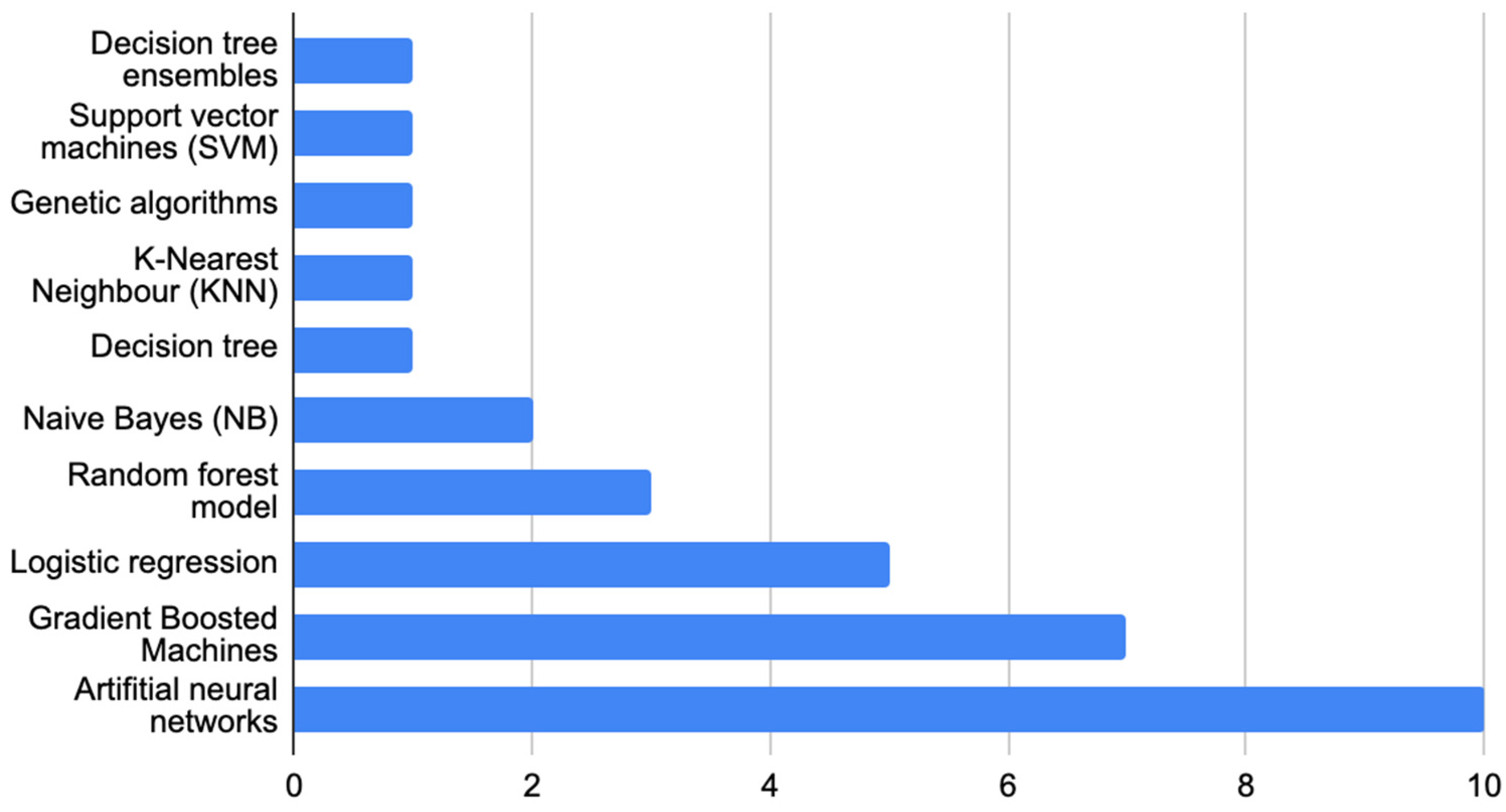
In recent studies, different classification methods have been employed to predict customer behaviour (see Figure 1). A significant portion of the recent literature has utilised neural network-based models. Fabra et al. (2020) developed a neural network-based model to predict the user profiles of anonymous session data. Koehn et al. (2020) proposed a recurrent neural network (RNN)-based model to predict conversion rates from clickstream data. Requena et al. (2020) developed two types of conversion prediction models based on gradient-boosting machines (XGboost) and neural network frameworks. In Requena et al.’s (2020) study, different types of clickstream sequences were compared and two modelling approaches were proposed: first, analysing full sequences of clickstream data, and second, early-stage conversion probability prediction while analysing only part of each sequence. Guo et al. (2019) proposed the Deep Intent Prediction Model (DIPM) based on an attention-based neural network framework. Cui et al. (2018) modelled customer online behaviour, including semantic customer data from search engines and the authors’ applied recurrent neural network (RNN) together with a convolutional neural network (CNN) for behaviour modelling and Monte Carlo simulation to predict conversion in future sessions. Earlier applications of neural network frameworks can also be found in the literature (Sheil et al. 2018; Toth et al. 2017; Hidasi et al. 2015; Wu et al. 2015).
Logistic regression models have been widely used for online behaviour prediction (Nishimura et al. 2018; Lo et al. 2016; Qiu et al. 2015; Van den Poel and Buckinx 2005), but in recent studies, they have been less commonly employed. Recently, gradient boosting machines (GBM) (Lee et al. 2021; Dou 2020; Requena et al. 2020; Song and Liu 2020; Wang et al. 2018) and random forest models (RFM) (Esmeli et al. 2021; Song and Liu 2020; Joshi et al. 2018) have gained popularity for predicting online behaviour. Other modelling techniques have also been used in the literature for the task of online purchase prediction by Esmeli et al. (2021), Song and Liu (2020), Turčanik (2020), Jia et al. (2017), Suchacka et al. (2015), Montgomery et al. (2004) and Kim et al. (2003).
A review of related studies reveals that there is still a lack of coverage in the scientific literature regarding personalised conversion prediction models that can customise predictions for individual customers based on demographic, economic, or financial data. Additionally, the analysis of conversion prediction models for the lending industry has only briefly been covered; however, as lending products are tightly connected to counterparty risk, user behaviour when purchasing these products may differ significantly from that when purchasing other e-commerce products. Moreover, researchers have not yet investigated the conversion prediction issue for OLCB platforms. Given the limitations of the current state of research, we aim to advance the state of the art by proposing the conversion, i.e., acceptance, prediction models for the online loan comparison and brokerage (OLCB) platforms that incorporate relevant personal data. For this reason, it is appropriate to discuss the theoretical background for evaluating binary classification models.

2.2. Theoretical Foundations for the Evaluation of Binary Models

According to the content of analytical information, the methods for evaluating the discriminatory power of a binary model can be divided into two types: (1) methods that show the discriminatory properties of the model at a selected cut-off point, and (2) methods that show the overall discriminatory properties of the model regardless of the selected cut-off point. Below, these two types of evaluation methods are analysed separately.

2.2.1. Evaluation of a Model’s Discriminatory Power at a Selected Cut-Off Point

Let us say that OLCB platform clients are evaluated by a conversion prediction model. The model assigns each potential customer a rating R, and it is assumed that the higher the rating is, the greater is the probability that the customer will take advantage of loan offers. In binary classification, in order to divide customers into “good” and “bad” categories, a cut-off point C is established. It is assumed that clients with R ≤ C are unlikely to take advantage of offers, and conversely, customers with R > C are likely to take advantage of loan offers. Ideally, the model will assign R ≤ C to all customers who do not take advantage of offers, and conversely, R > C to customers who seek to take advantage of loan offers. However, in practice, ideal models are rare, and so the model will assign some “good” clients to the “bad” category and vice versa. In other words, when the model is applied and the cut-off point C is chosen, there can be four types of responses:
  • Customers to whom the model assigned R ≤ C and who did not take advantage of loan offers are considered correctly classified as “bad” customers (true negatives, TN);
  • Customers to whom the model assigned R > C and who did take advantage of loan offers are referred to as correctly classified “good” customers (true positives, TP);
  • Customers who were classified as “bad,” with R < C, but who took advantage of the offered loans are considered wrongly assigned to “bad” (false negatives, FN). This model error is also called a type I error;
  • Customers for whom the model assigned R > C, but who did not take advantage of loan offers, are referred to as wrongly positively classified clients (false positives, FP). This model error is called a type II error.
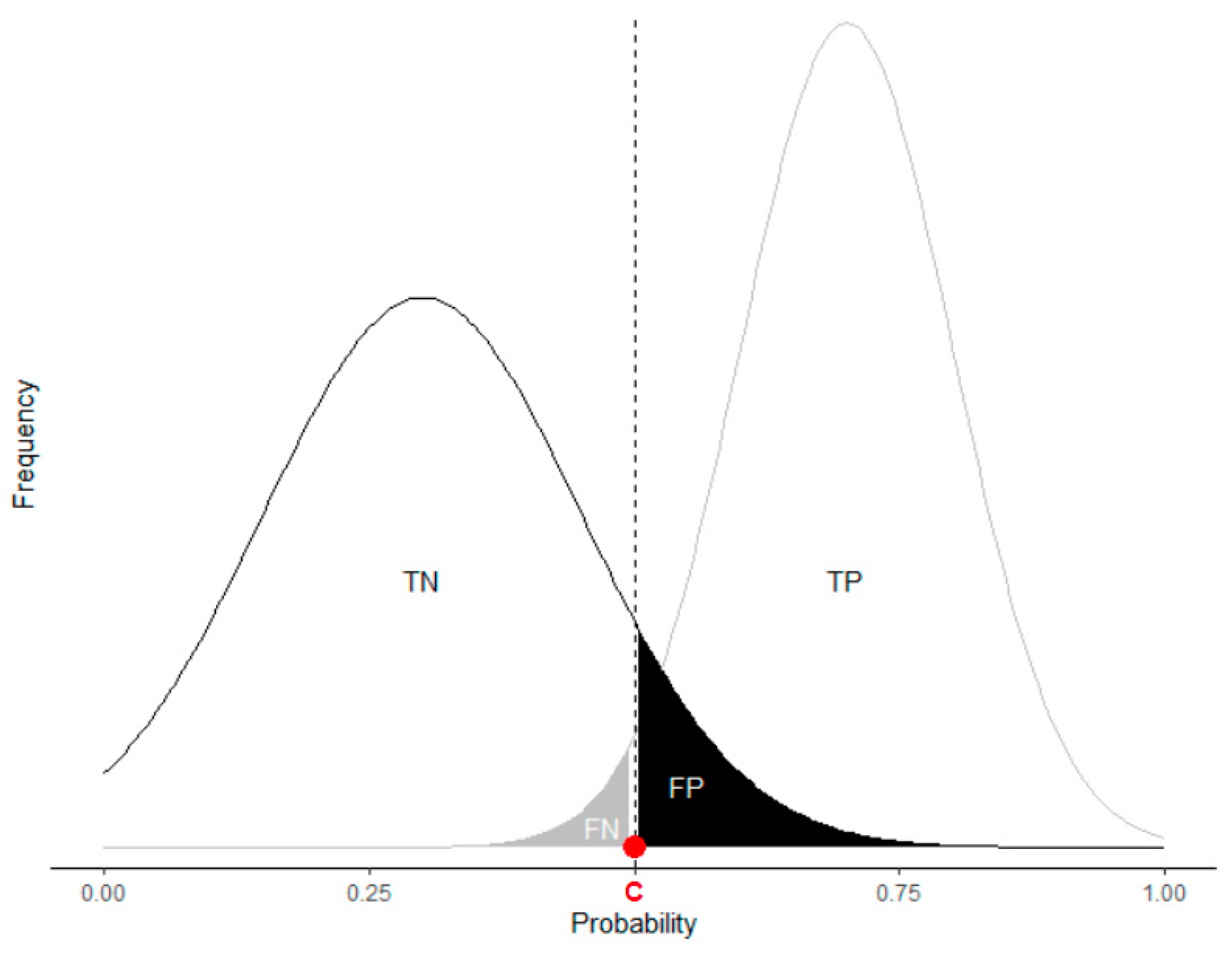
In Figure 2, two hypothetical customer distributions, “bad” and “good,” are shown, starting from the left. The X-axis represents the scale of the rating assigned by the model, and the Y-axis represents the frequency of customer distribution. By choosing the cut-off point to be point C at 0.5, the parts of the distribution representing correctly and incorrectly classified customers are visible. From Figure 2, it is clear that by changing the value of point C, we can reduce the proportion of FP or FN errors, but this would usually be done at the expense of the opposite error; i.e., by setting a more conservative point C value, such as 0.4, the proportion of incorrectly classified “bad” customers would decrease, but a larger portion of “good” customers would be lost (Sobehart and Keenan 2001).
Further, in analysing the properties of the model, for simplicity, Figure 2 can be transformed into confusion matrix form (Table 1), which is widely applied in the scientific literature when analysing binary classification problems.
The columns of Table 1 correspond to the predicted number of “good” and “bad” customers by the model, while the rows represent the actual customer conditions. Accordingly, the intersections of the rows and columns show the discriminative power of the model that has been discussed, i.e., TP, TN, FP, FN. The contents of the classification matrix enable the calculation of indicators that show the discriminative properties of the model at the selected cut-off point.

2.2.2. Model Discriminatory Power Assessment without Considering the Cut-Off Point

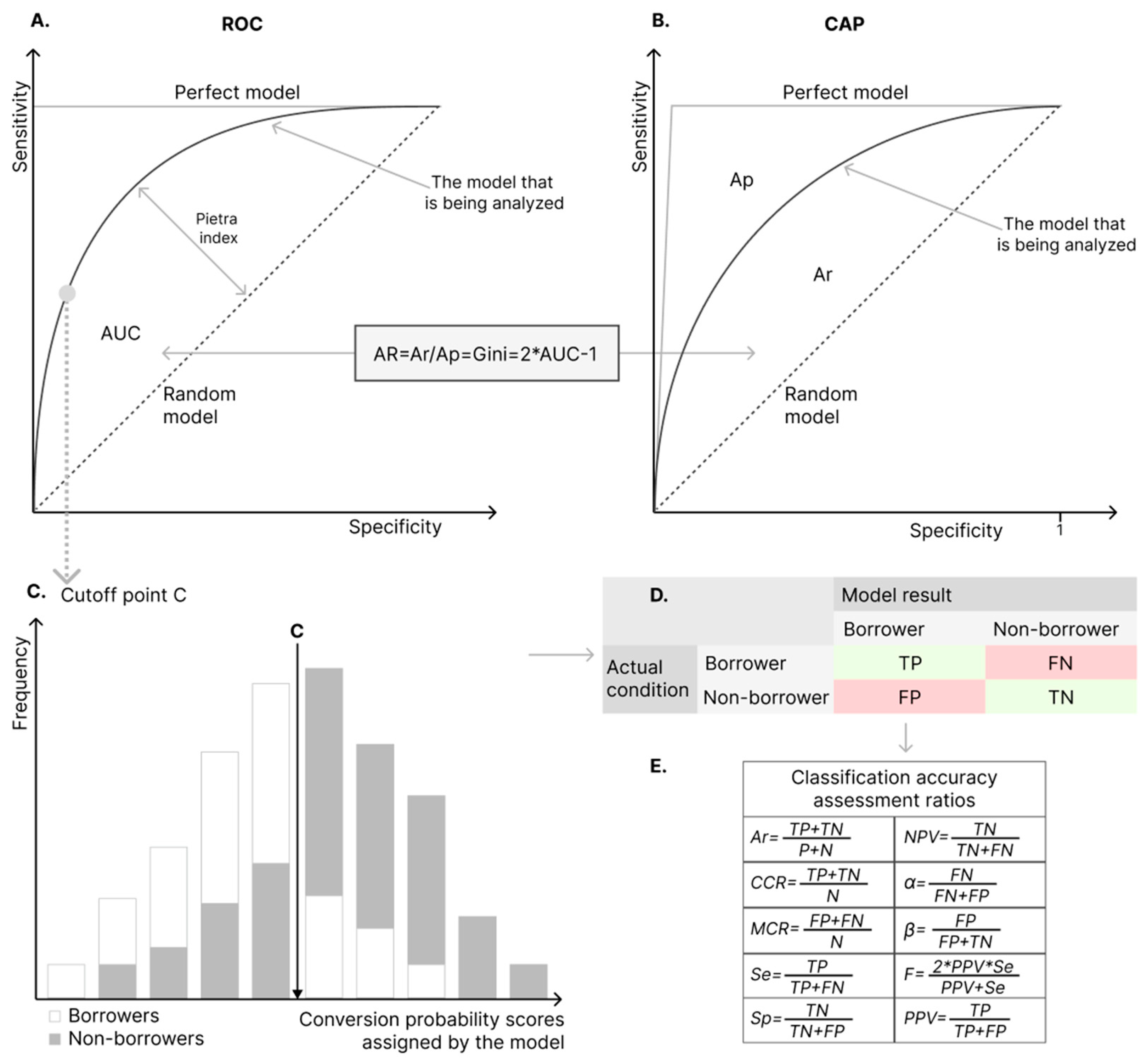
The receiver operating characteristic (ROC) curve is created for each possible cut-off point C, determining (1) the portion of “good” customers correctly classified by the model, i.e., the specificity of the model, which is characterised by the size of the X-axis, and (2) the portion of “bad” clients correctly identified by the model, i.e., the sensitivity of the model, which is indicated on the Y-axis of the graph. In this way, the graph shows a summary of the model’s discriminatory abilities in terms of first and type II errors for each possible cut-off point C (see Figure 3A).
The closer the ROC curve is to the upper left corner, the more the model is considered to be of higher quality, and conversely, the closer the curve is to the line of the graph’s diagonal (see Figure 3A, dotted line), the less discriminatory power the model has. A model whose ROC curve is close to the diagonal line is considered to be naive (random or coincidental).
The area under the ROC curve (AUC) summarises the discriminatory abilities of the model quantitatively. The AUC varies from 0 to 1, and the closer the model’s AUC is to 1, the more reliable it is considered. In other words, if the model’s AUC is 1, the model classifies “good” and “bad” customers with 100% accuracy. As mentioned, such models are impossible in practice.
The cumulative accuracy profile (CAP) curve, also known as the Gini curve, Lorenz curve, or power curve, is also used to assess the discriminatory abilities of the model. When creating the CAP curve, customers are first ranked according to the rating assigned by the model, from the riskiest to the least risky. The cut-off point is considered to be the rating assigned by the model. The Y-axis of the graph shows the sensitivity (Se) of the model, and the X-axis shows the cumulative share of customers (Špicas 2017; Irwin and Irwin 2012; Dzidzevičiūtė 2013) (Figure 3B).
It can be stated that the methods for evaluating the discriminatory power of a model— ROC and CAP curves, AUC, AR metrics, the Pietra index, and accuracy metrics—are all related by a linear relationship. This relationship is illustrated in Figure 3.
  • In Part A of Figure 3, the ROC curve is depicted, with the area under the curve being the AUC and the distance from the diagonal representing the naive model to the evaluated model’s ROC curve being the Pietra index.
  • In Part B of Figure 3, the CAP curve is shown, with the area under the curve being the A R , the area under the perfect model curve being the A P , and the naive model’s CAP curve being represented by a dotted line.
  • A formula is provided between the ROC and CAP curves (Figure 3A,B) demonstrating the linear relationship between the two methods.
  • In the ROC curve (Figure 3A), a hypothetical cut-off point C is shown, with its “bad” and “good” customer classification divisions (Figure 3C), the portions of customers correctly and incorrectly classified—which can be transformed into a classification matrix (Figure 3D)—and accuracy metrics can be calculated from the matrix (Figure 3E).
In scientific literature, the methods of evaluating a model are usually applied in two stages: first, a preliminary evaluation of the model is carried out, and second, backtesting of the model is conducted. The same methods discussed in this section are used for evaluation. The difference is that in the preliminary evaluation of the model, the cut-off point is determined expertly (usually by setting it at 0.5), and the model’s features are evaluated on a test sample formed from the initial sample available. In backtesting, the model is tested in a “production environment,” i.e., it is applied under real conditions (e.g., by simulating the model’s application on a platform for which it has been created), using available data and quantifying the cut-off point.
3. Methodology of Development of Statistical Conversion Prediction Model

3.1. Data Preprocessing

3.1.1. Definition of Dependent Variable and Seclusion of Non-Homogenous Cases

Defining the dependent variable in a model involves answering two questions. The first is: what characteristic or set of characteristics could characterise the analysed customer as “good” or “bad”? The second is: what is the optimal customer’s behaviour observation period?
In this paper, those loan applications in which the client selected one of the loan offers presented to them are considered as converted, i.e., “good” applications. The criterion that allows an application to be classified as a “good” application is that the customer expresses a desire to use one of the loan offers by performing two actions: (a) clicking the button “Select” on the loan offer card, and (b) reviewing the details of the loan offer and clicking “Proceed to the contract”. It is important to note that some customers who are classified as “converted” (“good”) may not ultimately receive a loan due to the KYC (know your customer) procedures of the lender, the customer’s inability to perform underwriting procedures, or the loan being denied after additional credit risk assessment.
The essence of determining the optimal customer’s behaviour observation period is the identification of a period during which the conversion probability is significant. There are two main methods for the retrospective analysis of behaviour patterns: case study and cohort analysis (Song and Chung 2010). Cohort analysis is often used to achieve this goal in cases of development of binary models (Špicas 2017; Špicas et al. 2015). To conduct cohort analysis on loan offer selection, a model creation dataset was employed in this study.
Additionally, in order to more accurately define the predicted event, an additional verification of the sample of “bad” customers was performed, asking the following questions:
  • Did the customer intend to take a loan?
  • Did the customer make a mistake in selecting the loan product? That is, did they actually need a consumer loan (not a mortgage loan or leasing)?
  • Did the customer decline the loan because they received a better loan offer outside the platform?
Answers to these three questions were obtained by analysing the reasons for the rejections of applications and comments written by customer service managers in the studied platform’s CRM (customer relationship management system) system. Customers who did not have the intention of taking a loan, indicated a wrong product, or received a superior loan offer outside the platform have been excluded from the sample as they are not homogeneous.

3.1.2. Data Normalisation

The ranges of the variables used in our analysis differed a lot. To appropriately use some machine learning and neural network techniques, it is necessary to unify the ranges of features. All numerical variables were normalised using the following formula:
x n o r m a l i s e d , i = x i x m i n x m a x x m i n .
Here, x n o r m a l i s e d , i is the normalised value of variable i and x m i n is the minimum value of x i . By using this method, we rescaled the range of all numerical features to the interval between 0 and 1. Similarly, it is necessary to prepare all the categorical data before using statistical and machine learning techniques. The one-hot encoding method was used to transform all the categorical and Boolean variables into numerical expressions of 0 or 1.

3.1.3. Class Imbalance Problem

Our original dataset was highly imbalanced, with 16,059 customers who had selected the loan offer and 9616 customers that rejected the loan offers. To deal with the class imbalance problem, we used three different sampling methods: Random Oversampling, Random Undersampling, and the Synthetic Minority Oversampling technique (SMOTE). Random Oversampling creates new samples by randomly selecting observations from the minority class with replacement and adds them to the training dataset. Using this technique, we increased the number of observations from the minority class to be equal to the majority class observations. On the other hand, Random Undersampling randomly selects examples from the majority class and deletes them from the training set until the number of observations becomes equal to the number of observations in the minority class. SMOTE technique (Chawla et al. 2002) is another method that helps to deal with class imbalance problems. This method artificially generates new observations for the minority class using the nearest neighbours method. Moreover, the majority class observations were also undersampled, leading to a balanced dataset. The machine learning method’s performance using resampled training datasets will be compared with its performance the original training dataset, allowing us to test what statistical improvements can be achieved by implementing sampling techniques.

3.2. Selection and Inclusion of Independent Variables in the Model

First, a list of possible independent model variables that could characterise each applicant was compiled. At this stage, 24 independent variables were included in the study. It was appropriate to divide the data that could be collected about the customers on the OLCB platform into four groups of independent variables, i.e., independent variables characterising (i) each customer’s behaviour on the analysed platform, (ii) demographic characteristics, and (iii) financial characteristics, and (iv) the course of loan offerings on the platform (competition).
Second, in order to ensure that the remaining independent variables in the final sample did not have strong interdependence and covered different analytical information in content, and so that the logit regression equation did not face the problem of multicollinearity, before including the independent variables in the model, it was necessary to perform correlation calculations for each pair of variables. If the correlation coefficient of a pair of variables exceeded 0.7, i.e., there was a strong or very strong correlation, the removal of the less significant variable from the model for further analysis was considered. The correlation was also evaluated to ensure it was not random, i.e., that the p-value < α = 0.05.
Third, the discriminatory power of individual variables was analysed and, fourth, backward stepwise regression was applied in forming the final set of independent variables for the model. The third and fourth steps were carried out in forming the logistic regression model.

3.3. Classification Algorithms

3.3.1. Logistic Regression

A logistic regression model is formed by calculating the coefficients of the selected independent variables. As noted in various studies (Yap et al. 2011; Nikolic et al. 2013; Megan and Circa 2014; Sorin 2015), logistic regression is a widely used statistical method for examining the relationship between a dichotomous outcome (Y = 0 or Y = 1) and a set of independent variables. The logistic regression equation is presented as follows:
A c c P = P Y = 1 = 1 1 + e z ,   w h e r e   z = α 1 + β 1 X 1 β n X n ,
where P (Y = 1) is the probability of the acceptance probability (AccP = probability that the customer will take advantage of the proposed loan offer, i.e., that they are a “good” customer).
Thus, the objective of a logistic regression model in conversion prediction is to determine the conditional probability of a specific applicant belonging to a class (“good” or “bad”) given the values of the independent variables of that credit applicant. For this study, the logistic regression was used to model the event Y = 1 (“good”).
A logistic regression model must meet certain requirements. These requirements include a chi-square criterion of the p-value being less than 0.05, as well as the McFadden R-squared, Cox and Snell R-squared, and Nagelkerke R-squared values being greater than 0.2. By checking for these requirements, one can be confident in the validity and usefulness of a logistic regression model (Kanapickienė and Špicas 2019).

3.3.2. Random Forest

Random Forest is an ensemble machine learning method for classification and regression that was first developed by Breiman (2001). Random Forest is an extension of another ensemble method called Bagging. Like Bagging, it works by constructing multiple decision trees on bootstrapped training samples and aggregating the predictions of those trees to get a more accurate final prediction and control over-fitting (Esmeli et al. 2021; Joshi et al. 2018). Instead of using all available feature variables as in Bagging, Random Forest algorithm randomly selects a subset of m predictors from the full set of p predictors (m < p). In the case of one powerful predictor existing in the dataset, the bagged decision trees could look very similar because all of the trees would be highly correlated. Random Forest overcomes this issue by taking only a subset of predictors, and this process is called decorrelation of the trees. After building numerous uncorrelated decision trees in the forest, the algorithm uses majority voting to decide to which category a given observation belongs. This method results in a high degree of accuracy and stability, and is especially useful for complex and non-linear data patterns.

3.3.3. Extreme Gradient Boosting (XGBoost)

XGBoost is an open-source machine learning library for gradient boosting trees that is commonly used for classification and regression tasks. It was developed by T. Chen and C. Gusterin and was first released in 2016 (Chen and Guestrin 2016). XGBoost has been widely adopted by researchers and industry practitioners due its ability to effectively capture the dependencies of complex data. It also uses extensible learning systems to learn from large data sets and get models (Song and Liu 2020).
Both Random Forest and XGBoost build models based on multiple decision trees. However, the process of “building” is the site of the main difference between those algorithms. Random Forest uses bagging to build all decision trees at once. On the other hand, XGBoost constructs an ensemble of decision trees using a gradient boosting algorithm to build trees in order to minimise the loss sequentially. In addition to gradient-boosting decision trees, Chen and Guestrin (2016) suggested adding a regularisation (penalty) term to the loss function to avoid possible overfitting:
L ( f ) = i = 1 n Ψ ( y i ^ , y i ) + k = 1 K Ω ( δ k ) .
Here, y i is the prediction of the i-th observation at the K-th boost (tree), Ψ () is the lost function to measure the difference between the prediction and the reference label, and Ω ( δ k ) is the regularisation term. This regularisation term can be expressed as follows:
Ω ( δ ) = γ T + 1 2 λ w 2 .
Here, γ is the complexity term, T is the classification’s number of leaves in the tree, λ is the penalty parameter, and w 2 is the output of each leaf node. Additionally, XGBoost applies second-order Taylor approximation in the loss function, and this is another way it in which it differs from gradient-boosted decision trees. More details about this algorithm can be found in Chen and Guestrin (2016).

3.3.4. Artificial Neural Networks (ANN)

Artificial Neural Networks (ANNs) consist of three main layers: input, hidden, and output layers. The more hidden layers are used, the more complex relationships may be modelled. A feed-forward neural network will be used in this process. In a feed-forward network, the information is carried forward from input variables through connected neurons in the middle (hidden) layers and finally to the specified output layer. Each neuron processes its inputs and transfers its output value to the neurons in the next layer. Each neuron processes its inputs and transfers its output value to the neurons in the next layer. Initially, these neural connections are assigned with random weights, and then, during the training process, the model adjusts the weights (Lee et al. 2021). The output value of hidden neuron i is calculated by applying activation function f ( 1 ) :
h i = f ( 1 ) ( b i ( 1 ) + j = 1 n W i j x j ) .
Here, W is the weight matrix and W i j denotes the weight connecting input j to hidden neuron i. In a similar way, the output of the output layer is computed by the following equation:
y = f ( 2 ) ( b ( 2 ) + j = 1 n h v j h j ) .
Here, n h is the number of hidden neurons and v denotes the weight vector, so that v j is the weight that connects hidden neuron j to the output neuron. In the case of binary classification, f ( 2 ) is a sigmoid activation function. More details about ANNs can be found in Bishop (1995).

3.3.5. Support Vector Machines (SVM)

Support Vector Machines (SVM) are a class of supervised machine learning algorithms used for classification that were invented by Cortes and Vapnik (1995). SVMs try to find the optimal hyperplane that separates classes by maximising the margin between the closest data points of different classes. These closest points are called support vectors (Huang et al. 2018). Since the behavioural and financial characteristics of customers cannot often be linearly separated, SVM analysis will include a radial basis kernel in this work. Based on Li et al. (2013), the classifier function of SVM for binary classification can be expressed as follows:
f ( x ) = s i g n ( i = 1 M α i y i K ( x , x i ) + b ) ,
using training dataset D = { x i , y i } , where x i   R m is the independent variable and y i   { 1,1 } is the target class, α i is the Lagrange multiplier, and K ( x , x i ) is the kernel function of the two vectors. In our work, radial basis function will be used as a kernel function, the expression of which is K ( x , x i ) = e ( γ x x I 2 ) . The SVM algorithm is discussed in more detail in Cortes and Vapnik (1995).

3.4. Model Evaluation Methods

In recent scientific studies, classification matrices have commonly been used to evaluate the reliability of binary models, and classification accuracy indicators are calculated from their data. The graphical analysis method for ROC curves is also often applied, and its results are quantitatively summarised by the AUC indicator, which shows the area under the ROC curve (Špicas 2017). The formulas for classification accuracy indicators are provided in Appendix A (Table A1). The table below (see Table 2) shows the model evaluation methods used in this study. The cut-off point was expertly set at 0.5. Such a decision was based on the experimental setup of our study. We used five different models and four scenarios involving sampling techniques. These summed up to 20 different experiments, which would have required setting 20 different optimal cut-off points. However, a variety of cut-off points would not allow us to compare the models homogeneously and for that reason the cut-off point was set at 0.5 for all the experiments.

4. Model Creation and Empirical Results

4.1. Setting Optimal Loan Offer Monitoring Time

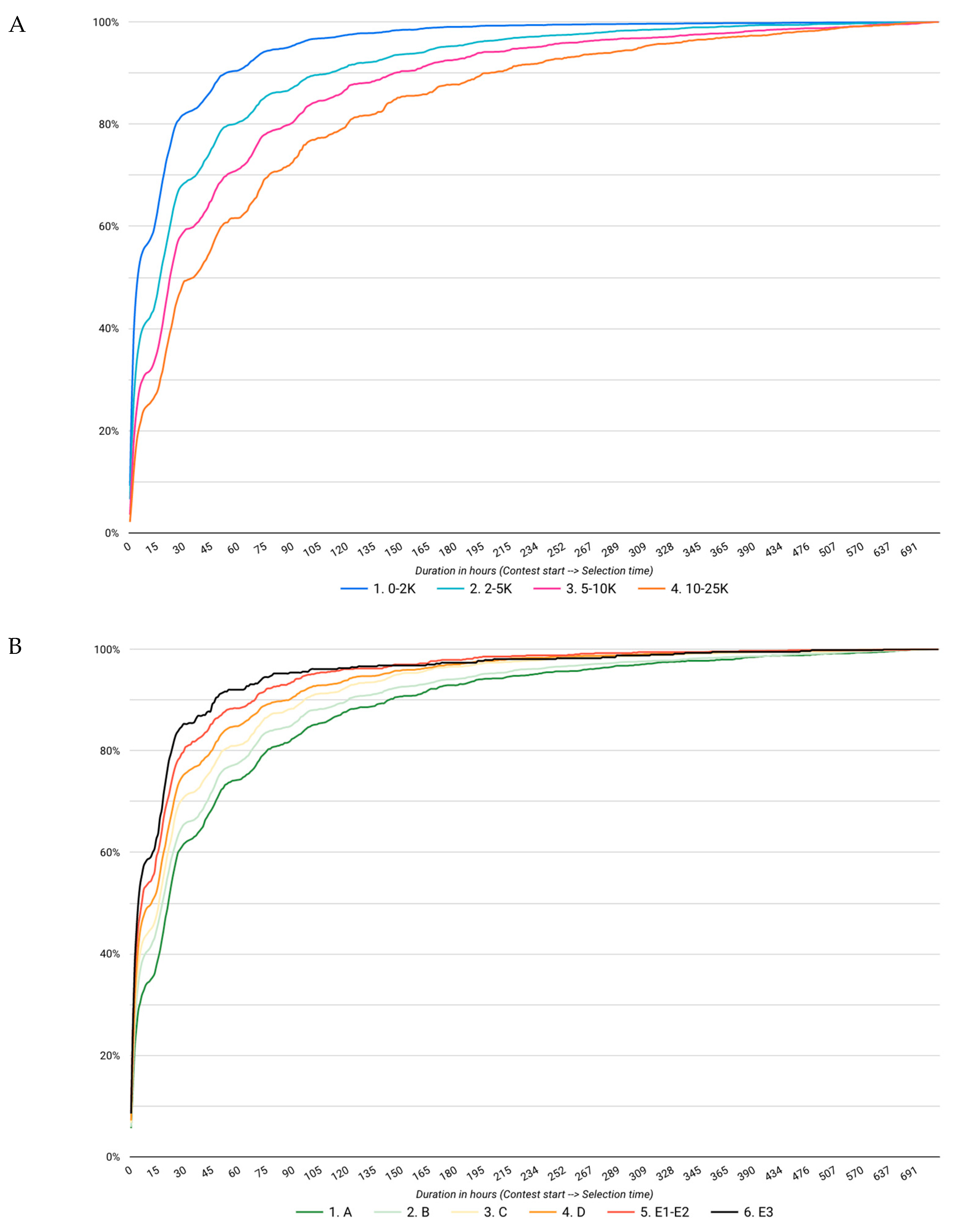
In order to quantitatively determine the optimal loan offer monitoring period, the data from LCP operating in Lithuania for the period from 1 September 2019 to 1 September 2022 was used for the study, providing a total of 16,059 contests wherein customers had chosen loan offers. First, by forming cohorts of loan offers presented in different periods, the chosen loan offer indicators were displayed (see Figure 4). In order to convey a more complete picture of the maturity of loan offers, a 1000-h period was analysed.
The aim was to investigate how customer decision-making behaviour differed when considering loan offers of different sizes, and the behaviours of customers in different credit risk segments were also analysed. Credit risk segments were created by grouping customers according to the credit rating calculated by Creditinfo Lietuva, a credit bureau operating in Lithuania. The assigned ratings indicated increasing credit risk from A (lowest risk) to E (highest risk). Rating E3 indicated customers whose insolvency probability (PD) according to credit bureau calculations was the highest—99%.
When analysing the behaviour of customers with different credit risks when choosing loan offers (Figure 4A), it can be seen that their decision-making times are proportional to their credit risk level—that is, the higher the customer’s credit risk is, the faster they make a decision to take out a loan. Similar results are seen when analysing customers considering different loan amounts (Figure 4B)—the larger the loan amount considered, the longer it takes the customer to make a decision.
The maturity cycle of loan offers is revealed in Figure 4. Periods are seen during which the curves of calculated offer selection indicators have clear growth potentials. Using this graphical information, the monitoring period was determined expertly. In this case, in the opinion of the authors, it was appropriate to set it at 180 h. Further in the study, taking into account the information structure of the model creation sample, the monitoring period was rounded to 168 h, i.e., one week. As can be seen from the cohort analysis, the selected monitoring period was suitable for analysing the behaviours of customers with different credit risks when choosing consumer loans of different amounts.

4.2. Formation of Model Training and Testing Samples

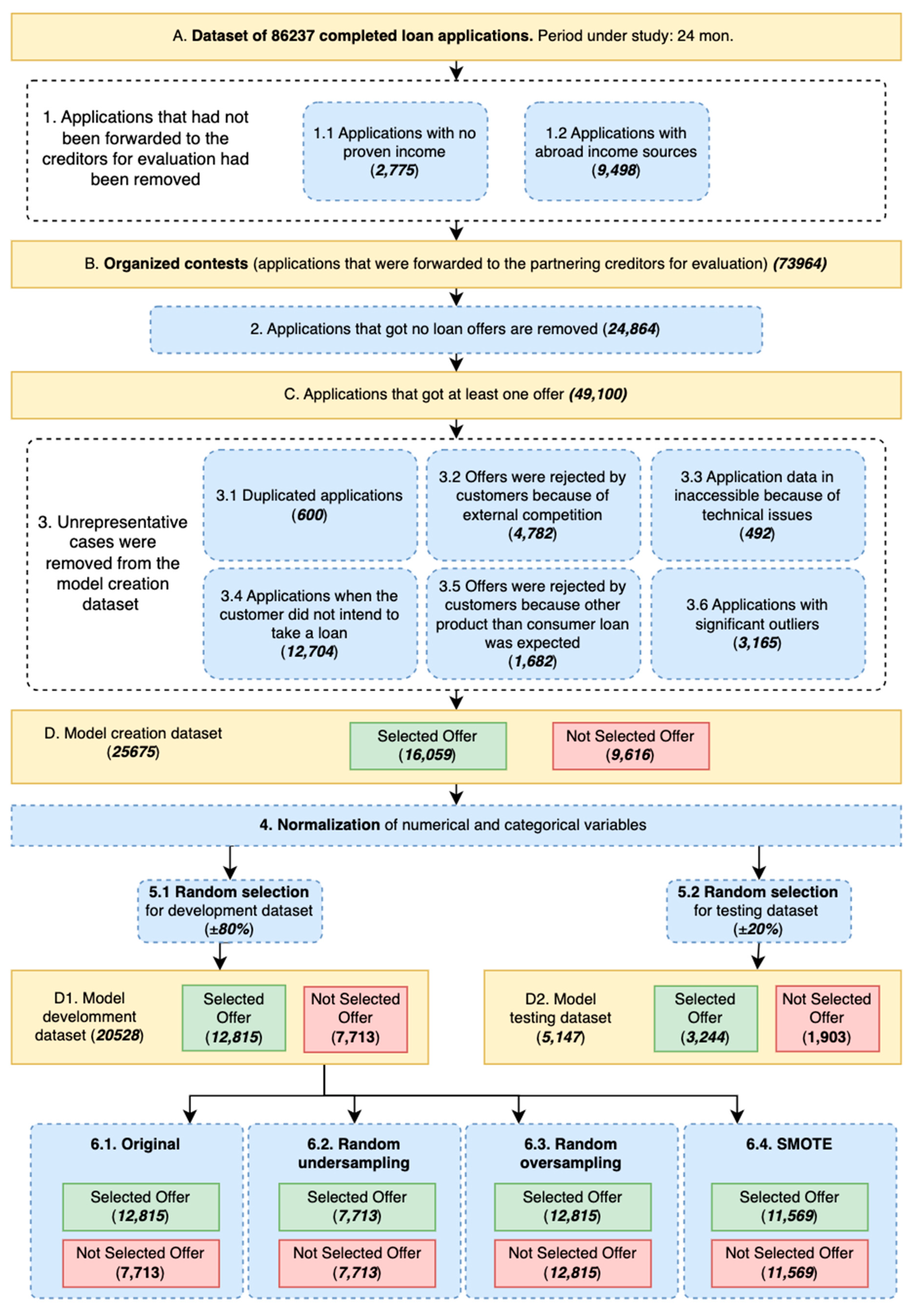
This stage of the study aimed to form the model creation, development, and testing sample from the initial data collection. The data on the activity of the chosen OLCB platform operating in Lithuania for the period from 1 September 2019 to 1 September 2022 was used for the study. The algorithm for model creation, formation, and testing the sample is presented in Figure 5: (i) shows the status of the data collection (Status A–D) and (ii) shows the data transformation/formation actions (Stages 1–6).
The initial data collection included all applications received during this period, which were 86,237 in number (Figure 5, Status A). The following actions were taken in forming the model development and testing samples.
First, in forming the study sample from the initial data collection, applications were removed that had not been submitted to creditors for evaluation (Figure 5, Stage 1). In this stage, applications of those clients who did not have assessable income and to whom, according to the relevant laws, consumer loans could not be granted, were removed. There were 2775 such applications (Figure 5, Stage 1.1). Additionally, in this stage, in order to form a homogeneous study sample in terms of client economic behaviour, 9498 applications submitted by clients working abroad were removed (Figure 5, Stage 1.2). The submission and further processing of these applications differed from those of regular consumer loan applications and were considered unrepresentative in the context of the study. After these two groups of applications were removed, 73,946 applications were submitted for the evaluation of the creditors (Figure 5, Status B).
Second, 24,864 applications that had received no loan offers were removed (Figure 5, Stage 2).
Third, from the applications that had received at least one loan offer (49,100, Figure 5, Status C), applications were removed that, in the authors’ opinion, did not characterise the applicants’ economic behaviours and were not suitable for inclusion in a homogeneous model creation sample. In this stage, the following cases were removed:
  • Duplicate client applications that had been removed manually, including applications submitted repeatedly by including a spouse or co-debtor—600 applications (Figure 5, Stage 3.1).
  • Clients who had reported receiving a better consumption loan offer outside the platform, i.e., from other creditors not participating in the platform’s activities—4782 applications (Figure 5, Stage 3.2).
  • Applications whose data became inaccessible due to technological issues—720 applications (Figure 5, Stage 3.3). The final sample for model creation consisted of 39,794 applications (Figure 5, Status D).
  • There were 12704 cases wherein clients had not taken advantage of the loan offers provided and explained that they were simply testing the platform’s functionality. In other words, the applicants had not had the intention of taking the loan.
  • Additionally, there were 1682 cases wherein clients claimed to have mistakenly chosen the loan product and actually needed a different type of loan, such as a home loan, business loan, or car leasing loan.
  • The applications that were excluded due to significant outliers equalled 3165 cases (Figure 5, Status 3.6).
This resulted in a total of 25,675 loan applications being considered for final model creation (Figure 5, Status D), of which each of 16,059 clients had utilised one of the loan offers received and 9616 clients had not used the offers.
Fourth, data—both numerical and categorical variables—were normalised (Figure 5, Step 4).
Fifth, the model creation dataset was randomly split into model development (80%) and model testing datasets (20%) (Figure 5, Stages 5.1 and 5.2).
Sixth, 4-model development datasets were produced by applying different sampling strategies (Figure 5, Stages 6.1, 6.2, 6.3, 6.4).

4.3. Selection of Independent Model Variables

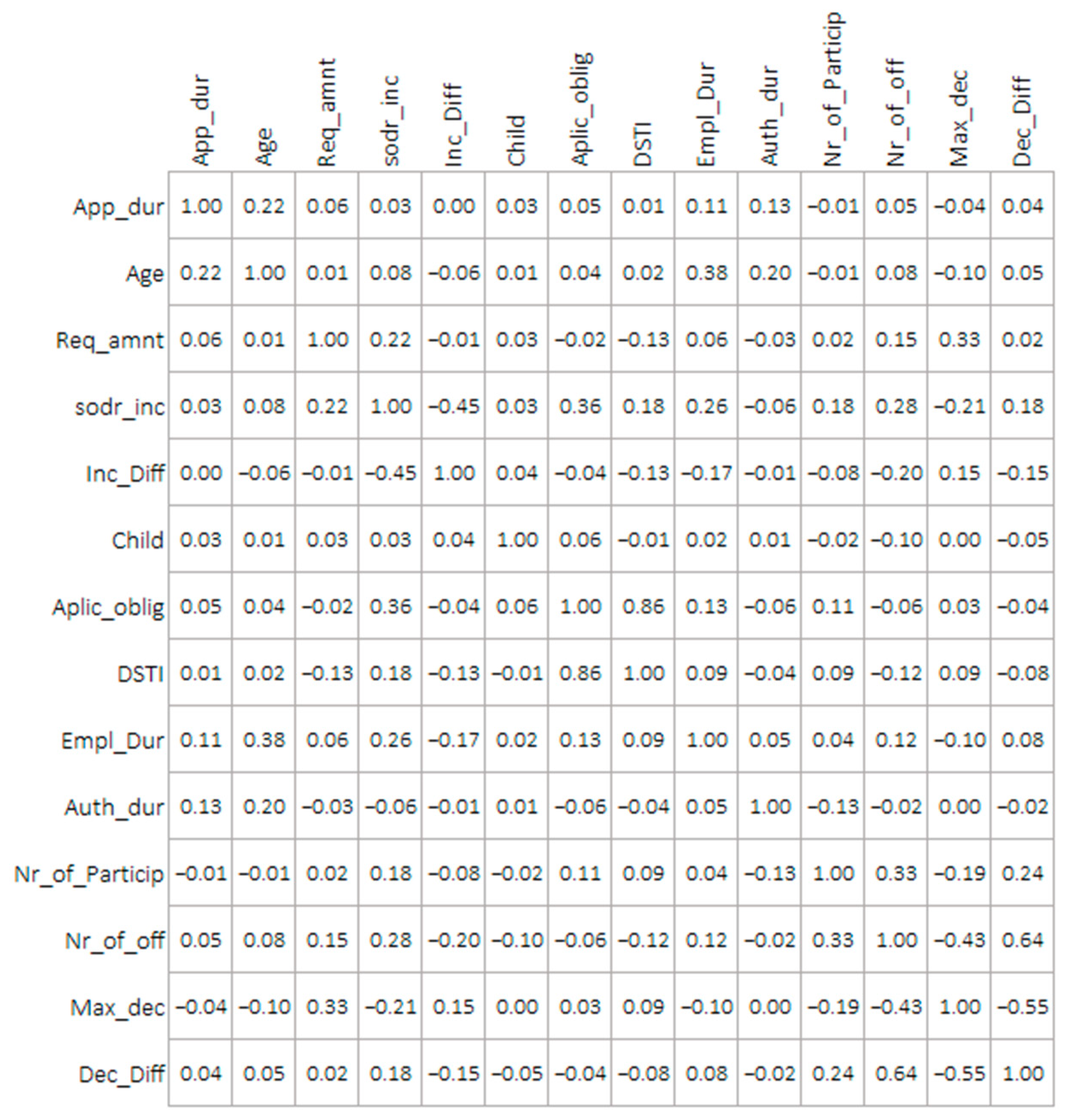
To ensure that the remaining independent variables in the final sample did not have strong interdependence and covered different analytical information in terms of content, a correlation calculation was performed for each pair of variables before incorporating the independent variables into the model (Figure 6). During the analysis, one indicator (see Appendix B, Table A2)— applicant commitments—was removed due to direct interdependence and strong correlation. This indicator had a strong correlation (0.86) with the DSTI (debt service-to-income) indicator due to their direct interdependence. Other positive and negative intercorrelations of indicators were weaker and economically justified, and these indicators are not linked by direct dependence relationships, and so it was likely that the correlation would not have a negative impact on the quality of the model.
Additionally, logistic regression for non-sampled training data (Figure 5, Stage 6.1) was used to remove non-informative (statistically insignificant) variables from further analysis. Four variables were removed based on their p-values being higher than 0.05: num_Of_Participants (p-value = 0.41), auth_duration_sec (p-value = 0.33), city_Classifier (p-value = 0.20), and Children (p-value = 0.17) (see Appendix B, Table A2).
The remaining variables were left for further analysis using other machine learning algorithms. Before the analysis of predictive performance of other machine learning techniques, we checked to see whether the coefficients from logistic regression followed economic logic (see Table 3). Based on the following results, we can now see that all the variables left in our analysis were associated with a Wald criterion (p-value) smaller than 0.10, showing that they were useful for predictions. Furthermore, the signs of the coefficients corresponded to economic logic.
A logistic regression model meets the following requirements (Table 4): (i) a chi-square criterion of a p-value of less than 0.05; (ii) McFadden R-squared, Cox and Snell R-squared, and Nagelkerke R-squared values of greater than 0.2. Therefore, we can be confident in the validity and usefulness of the logistic regression model.
Based on the information provided, it appears that our logistic regression model meets all the requirements outlined in Table 4. This means that the analysis of logistic regression coefficients can be confirmed to be appropriate.

4.4. Results

The objective of this section in the paper is to utilise and compare multiple machine learning algorithms for the purpose of predicting conversions on OLCB platforms. The comparative results of five machine learning algorithms are included. Specifically, logistic regression, random Forest, XGBoost, artificial neural network, and support vector machine methods were selected for this purpose.
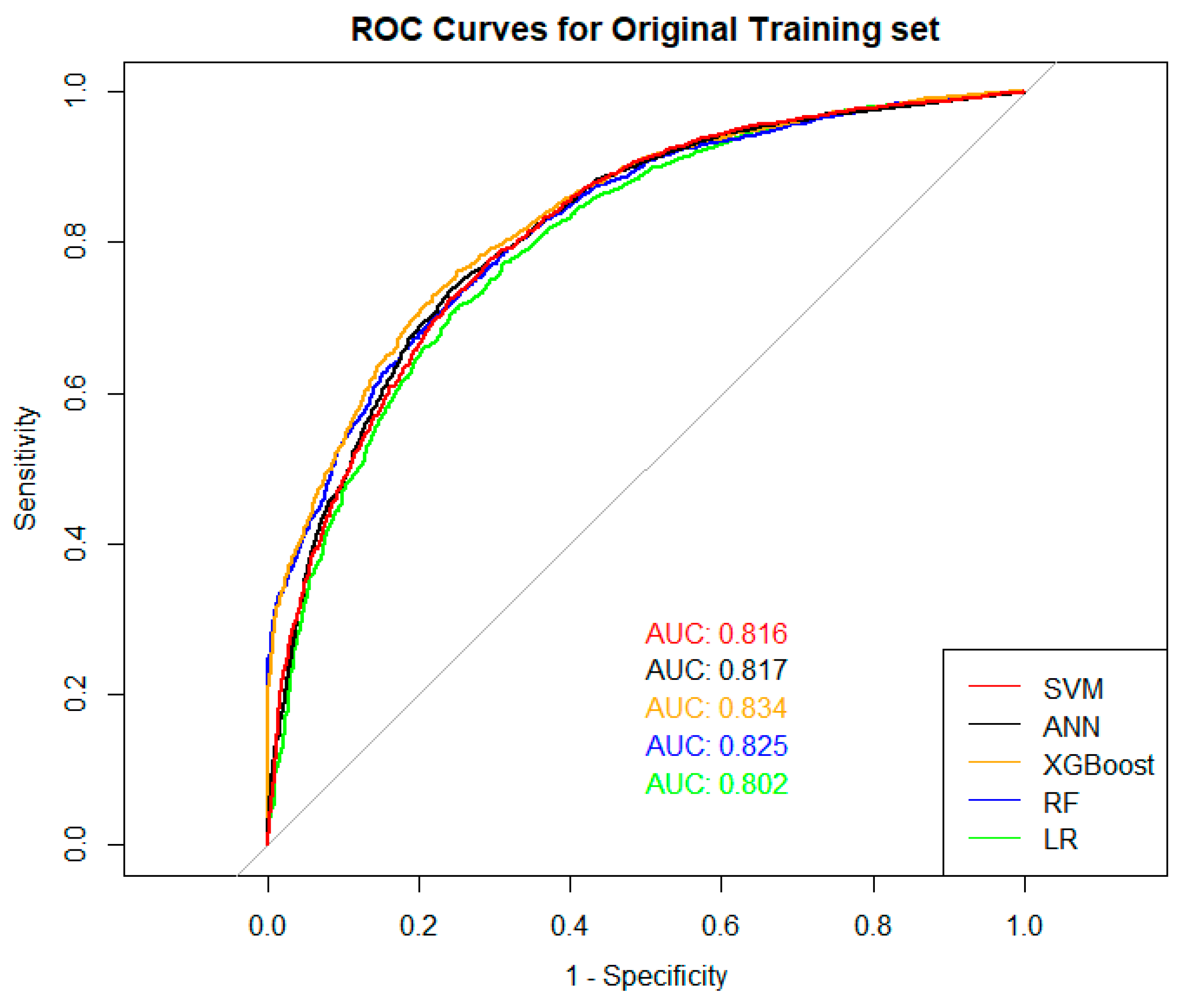
Firstly, the original non-sampled training data were utilised to evaluate the performance of four different evaluation metrics—AUC, Sensitivity, Specificity, and Accuracy. The findings, presented in Table 5, reveal that the Support Vector Machine was the most effective algorithm for Sensitivity, followed by XGBoost. In contrast, the ANN and Random Forest methods performed poorly in terms of Sensitivity. However, these algorithms demonstrated the highest Specificity, while Logit and SVM produced the lowest results. With respect to AUC, XGBoost performed exceptionally well, achieving an impressive score of 0.834 when using the original training dataset. Random Forest was the second-best algorithm for AUC, while Logistic Regression and ANN had the lowest AUC value —0.802. Moreover, XGBoost achieved the highest Accuracy of 0.763. Based on these results, it can be concluded that XGBoost is the most suitable machine learning algorithm for conversion prediction on the studied loan comparison platform, and will be used as a benchmark for comparing different sampling strategies.
Secondly, we examined how the predictive performance of classifiers varies when different sampling techniques are utilised. In our research, we applied the Random Oversampling, Random Undersampling, and SMOTE sampling methods in addition to comparing them to the original non-sampled training dataset. To assess the effectiveness of these sampling techniques here, we will utilise XGBoost as the benchmark algorithm, as it demonstrated the highest predictive power in the previous comparison of algorithms.
Table 6 displays the performance of the XGBoost algorithm when compared using various sampling techniques. The AUC measure results were relatively consistent across all sampling methods, with the highest score of 0.834 achieved using the original training dataset. For Sensitivity, the original training dataset yielded the most accurate results, with SMOTE being the second-best technique. The situation was different for the Specificity measure, as Random Oversampling and Random Undersampling were the two most effective sampling techniques, with Random Undersampling producing a score of 0.749. In terms of Accuracy, the original and SMOTE training datasets performed equally well, achieving a score of 0.763. Given that the performance of the sampling techniques did not significantly improve the XGBoost algorithm’s performance, it can be concluded that our original dataset did not experience a significant class imbalance problem and could be used for conversion prediction in the studied OLCB platform. Appendix C (Table A3) presents the results of all variations of applied modelling and sampling techniques.
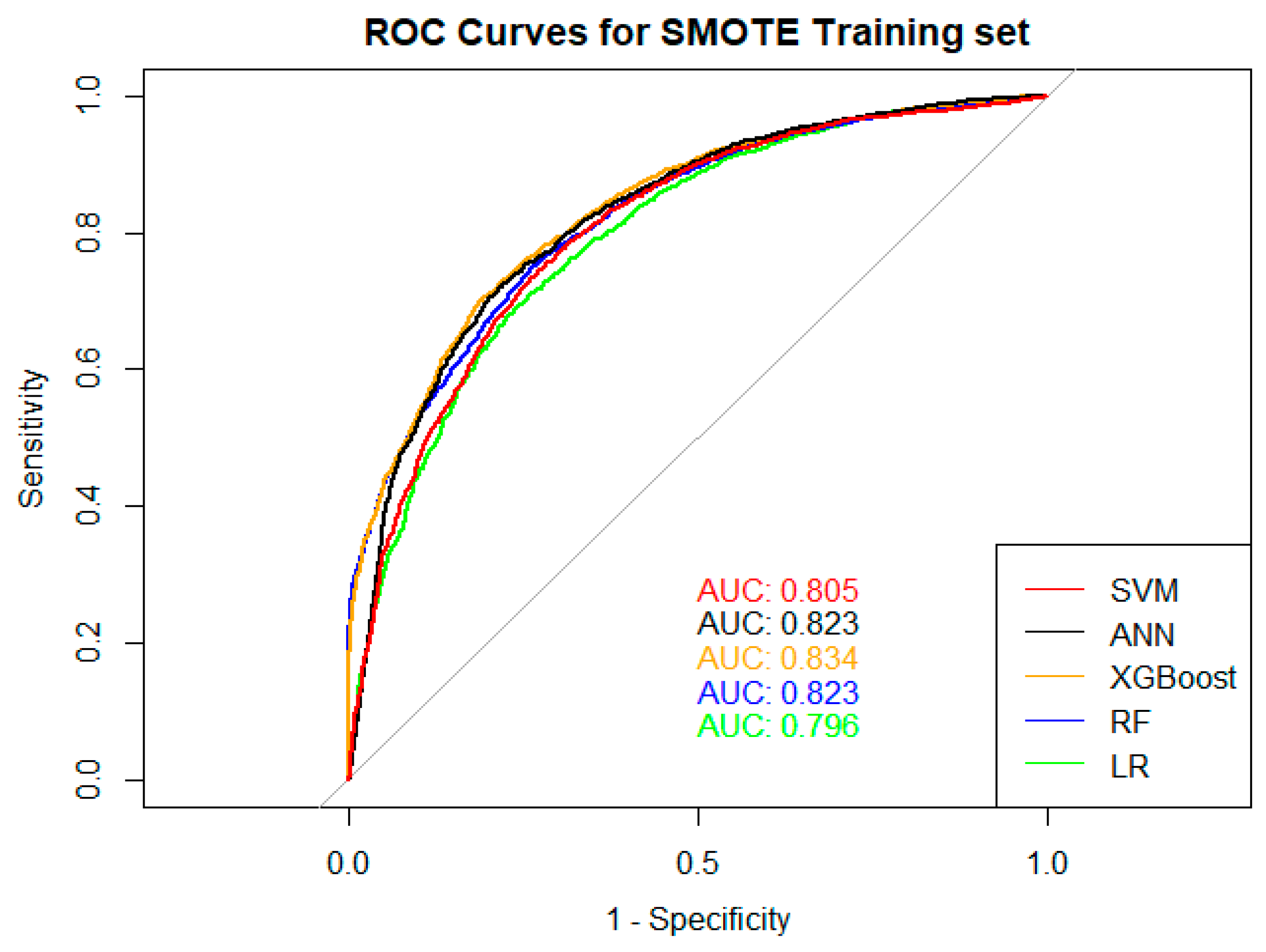
Lastly, we can compare the ROC curves of all the algorithms through four sampling methods (see Appendix D, Figure A1).

5. Conclusions

After conducting both theoretical and empirical research, the following conclusions can be drawn:
  • Based on a review of relevant scientific literature on conversion prediction, binary modelling, and two-sided markets, it can be concluded that a conversion prediction model would serve as a valuable technical tool for optimising the discovery mechanisms of a platform, controlling the competition between creditors, and improving the economic benefits of contest participation. Moreover, the model would help OLCB platforms improve customer satisfaction and minimise the risks of mismatching and misleading customers. In summary, a conversion prediction model has the potential to enhance an OLCB platform’s performance and benefit all parties involved.
  • In scientific literature, various classification methods have been used to validate binary models. These methods can be categorised into two types: those calculated without regard to a cut-off point, such as AUC, CAP, and Gini index, and those calculated at a specific cut-off point, including Sensitivity (Se), Specificity (Sp), Accuracy (Ar), Correct Classification Rate (CCR), Misclassification Rate (MCR), and Positive Prediction value (PPV). These classification accuracy ratios were employed in this study to evaluate the models.
  • The data on the activity of an OLCB platform operating in Lithuania for the period from 1 September 2019 to 1 September 2022 were utilised for the study. The dataset included 49,100 cases wherein at least one loan offer was presented to the customer. Based on this data, independent variables were created that covered the customer’s behavioural, financial, and contest characteristics. The model development dataset consisted of 20,528 cases: 12,815 cases when customer took the offer and 7713 when no offer was selected. Different sampling techniques were applied to address the class imbalance problem: original sampling, undersampling, oversampling, and SMOTE. Therefore, four model development datasets and one test dataset were formed.
  • For the selection of independent variables missing values, a correction matrix and stepwise regression was used to form the final set of independent variables. 14 variables were selected for model development.
  • Five different models were developed for each of the four types of datasets—normal sampling, Random Undersampling, Random Oversampling, and SMOTE. The models evaluated were logistic regression, support vector machine, artificial neural network, random forests, and XGBoost.
  • Based on AUC and Accuracy measures, XGBoost was found to be the most effective machine learning technique with an AUC of 0.834 and Accuracy of 0.763. When compared to other techniques, XGBoost performed the best on the original dataset. However, there were no significant differences observed when comparing sampling methods, as AUC measures across all techniques were highly stable. That being said, the original and SMOTE datasets demonstrated the highest level of accuracy at 0.763.
The main research limitations that must be taken into consideration include the following:
  • Country: This study was conducted in Lithuania, where the consumer lending industry operates under specific regulations. It is important to take into consideration that local regulations have a significant influence on the behaviours of both consumer lenders and customers. Moreover, the informational infrastructure of each country varies due to diverse regulations and industry practices implemented by local market regulators and credit bureaus. This means that the research data used in this study may be not available when building the conversion prediction models for OLCBs operating in other countries.
  • Product. This study focuses on the consumer lending industry. It is important to note that the behaviour of customers when purchasing other lending-related products may differ significantly when compared to their behaviour in the consumer lending industry.
Future research may focus on building conversion prediction models for OLCBs in other countries, considering their unique informational infrastructure. Additionally, it is imperative to incorporate data from open-banking sources.

Author Contributions

Conceptualization, R.Š., A.N. and R.K.; methodology, R.Š., A.N., R.K., D.V. and G.K.-S.; validation, R.Š., A.N., R.K., D.V. and G.K.-S.; formal analysis, R.Š., A.N. and R.K.; investigation, R.Š., A.N. and R.K.; data curation, R.Š., A.N. and R.K.; writing—original draft preparation, R.Š., A.N. and R.K.; writing—review and editing, R.Š., A.N. and R.K.; visualisation, R.Š., A.N. and R.K.; supervision, R.K. and R.Š.; project administration, R.K. and R.Š.; funding acquisition, R.Š., A.N., R.K., D.V. and G.K.-S. All authors have read and agreed to the published version of the manuscript.

Funding

This research has received funding from the European Regional Development Fund (project No 13.1.1-LMT-K-718-05-0010) under grant agreement with the Research Council of Lithuania (LMTLT). The project was funded as the European Union’s measure in response to the COVID-19 pandemic.

Data Availability Statement

Not applicable.

Conflicts of Interest

The authors declare no conflict of interest.

Appendix A

Table A1. Methodology of the Calculation of Model Evaluation Criteria.
RatioFormulaExplanationRatioFormulaExplanation
Ar T P + T N P + N Accuracy rate shows what portion of the analysed subjects were classified correctly.NPV T N T N + F N Negative Predictive Value (NPV) is the proportion of correct negative classifications among all negative classifications.
CCR T P + T N N Correct classification rate indicates the proportion of correctly classified customers compared to those classified as “bad”α F N F N + F P False negative rate is the ratio of false negative classifications, which is a measure of type I error.
MCR F P + F N N Misclassification rate shows the ratio of misclassified customers to those classified as “bad”β F P F P + T N False positive rate is the ratio of false positive classifications, which is a measure of type II error.
Se T P T P + F N Sensitivity ratio, also known as Hit ratio, is a metric that shows what portion of “bad” customers were correctly classified.F 2 P P V S e P P V + S e F-value is the harmonic mean of sensitivity and specificity.
Sp T N T N + F P Specificity, also known as False alarm ratio, is a metric that indicates what portion of “good” customers were correctly classified.BAS S e + S p 2 The metric reflects the overall accuracy of the model and is suitable for use in cases with low proportions of negative subjects (Harris 2015).
PPV T P T P + F P Positive Predictive Value is the proportion of correct positive classifications among all positive classifications.G-average T P + T P F N + T N + T N F P   The indicator shows the balance between model sensitivity and specificity (Tomczak and Zięba 2015).
It is important to note that both the classification matrix and the discriminant model analysis indicators presented in Table A1 characterise the model’s properties only at a certain cut-off point C. In order to generalise the discriminant properties of the model, graphical analysis methods such as ROC and CAP curves, which summarise the accuracy of the model across all C points, are used. The quantitative measure of CAP properties is typically summarised by the accuracy ratio (AR) indicator (see formula (A1)):
A R = A R A P = G i n i
In the formula, A R is the accuracy ratio, A R is the area under the CAP curve, and A P is the area under the perfect model curve. The accuracy ratio (AR) is equal to the Gini index (Pranckevičiūtė 2014). As can be seen from the provided definitions, there is a linear relationship between the AR and AUC indicators, which can be expressed mathematically as follows (Engelmann et al. 2003):
A R = 2 A U C 1
Another statistical method related to the ROC curve method is the Pietra index. This index shows the maximum distance from the diagonal of the naive model to the ROC curve of the analysed model (see Figure 3A). In statistical terms, this index is equivalent to the Kolmogorov-Smirnov test, which analyses whether two populations can be from the same distribution (Engelmann et al. 2003). In the case of the naive model, the Pietra index would be equal to 0. It is important to note that both the Pietra index and the KS indicator only analyse the maximum possible distance between the diagonal and the ROC curve.

Appendix B

Table A2. The process of selecting the final set of independent variables for model creation.
GroupVariable DescriptionVariableTypeStage 1Stage 2Stage 3Final Set of Model Variables
Missing ValuesCorrelationStepwise Regression
BehaviouralWas the offer selected? (Dependent var.)offer_SelectedBoolean++++
Duration of application filling processapplication_duration_secNumerical++++
Returning customer in 30 days?returning_30dBoolean++++
Customer authentication methodauth_MethCategorical++--
Duration of authentication processauth_duration_secNumerical++--
Time of day when the application receivedtime_ClassificatorCategorical++++
ApplicationAgeageNumerical++++
Requested loan amountreq_AmountNumerical++++
Personal or family loanapp_Applicant_TypeCategorical++--
Marital statusmarital_statusCategorical++++
GendergenderCategorical++++
Type of city of applicantcity_ClassifierCategorical++--
Number of children or dependantschildrenNumerical++--
FinancialTotal incomes of applicantappl_Income_Amount_TotalNumerical+---
Labor income of Applicant (from state database)aplic_Sodra_Sust_IncomeNumerical++++
Difference between the declared labor incomes compared to official incomes retrieved from governmental databaseincome_DifferenceNumerical++++
Monthly payment for existing financial obligationsaplic_ObligNumerical+---
DSTI ratio calculated from application datadsti_AplNumerical++++
Duration of existing employmentempl_Duration_MonNumerical----
ContestDuration of the contestauth_To_Cont_End_Dur_MinNumerical++--
Number of lenders participating in contestnum_Of_ParticipantsNumerical++--
Number of received loan offersnum_Of_OffersNumerical++++
Max. decency score of received offersmax_Decency_ScoreNumerical++++
Min. decency score of received offersmin_Decency_ScoreNumerical+---
Max. difference between the decency scores of offers receiveddecency_DiffNumerical++++

Appendix C

Table A3. Model evaluation criterias: comparison of on Logit, RF, Bagging, Xgboost, ANN and SVM classifiers on different class imbalance methods.
Logistic RegressionRandom ForestXGBoostANNSVM
Orig.RORUSmoteOrig.RORUSmoteOrig.RORUSmoteOrig.RORUSmoteOrig.RORUSmote
Ar0.7480.7320.7330.7290.7570.7610.7420.7380.7630.7520.7500.7630.7500.7510.7500.7520.7620.7430.7400.751
CCR2.6041.7581.7761.6982.3832.3631.6061.6672.6191.7781.7252.3022.4032.4152.5142.3212.8981.7861.7572.110
MCR0.8760.6420.6471.0260.7650.7410.5600.9500.8130.5880.5761.0200.8010.8000.8391.1110.9060.6180.6171.042
Se0.8660.7510.7540.7380.8490.8480.7220.7340.8740.7610.7500.8420.8470.8490.8580.8400.8960.7590.7530.814
Sp0.5480.7020.6970.7140.6010.6130.7750.7450.5740.7360.7490.6280.5840.5840.5650.6030.5330.7150.7180.645
BAS0.7070.7260.7250.7260.7250.7310.7490.7400.7240.7480.7500.7350.7160.7170.7120.7210.7150.7370.7360.729
MCC=AC0.4410.4430.4420.4410.4660.4760.4810.4660.4760.4850.4860.4820.4490.4520.4460.4570.4710.4640.4610.463
PPV0.7660.8110.8090.8150.7840.7890.8450.8310.7780.8310.8360.7940.7760.7770.7710.7830.7660.8190.8200.796
NPV0.7050.6230.6240.6150.7000.7030.6210.6220.7280.6430.6370.7000.6920.6950.7000.6880.7500.6350.6310.670
Alfa0.3360.5880.5800.6100.3930.4000.6780.6400.3350.6070.6300.4190.3850.3820.3570.4080.2760.5900.5990.473
Beta0.4520.2980.3030.2860.3990.3870.2250.2550.4260.2640.2510.3720.4160.4160.4350.3970.4670.2850.2820.355
F0.8130.7800.7810.7740.8150.8170.7790.7800.8230.7940.7910.8180.8100.8110.8120.8100.8260.7880.7850.805
G-average1.1891.2051.2041.2051.2041.2091.2241.2161.2031.2231.2241.2131.1961.1971.1931.2011.1951.2141.2131.208
ACP0.7210.7210.7210.7200.7330.7380.7410.7330.7380.7430.7430.7410.7250.7260.7240.7290.7360.7320.7310.731
AUC0.8020.8010.8020.7960.8250.8240.8270.8220.8340.8320.8330.8330.8020.8020.7950.8010.8160.8100.8100.805

Appendix D

Figure A1. Comparison of ROC Curves for SVM, ANN, XGBoost, RF, and LR Models with Different Sampling Strategies.
Risks 11 00138 g0a1aRisks 11 00138 g0a1bRisks 11 00138 g0a1c

References

  1. Agarwal, Sumit, and Marieke Bos. 2019. Rationality in the consumer credit market. In Handbook of US Consumer Economics. Cambridge, MA: Academic Press, pp. 121–39. [Google Scholar]
  2. Agarwal, Sumit, Souphala Chomsisengphet, Chunlin Liu, and Nicholas S. Souleles. 2015. Do consumers choose the right credit contracts? The Review of Corporate Finance Studies 4: 239–57. [Google Scholar] [CrossRef] [Green Version]
  3. Akimoto, Tomonari, and Fumiko Takeda. 2009. Price movements in the Japanese online home electronics market. Electronic Commerce Research and Applications 8: 28–36. [Google Scholar] [CrossRef]
  4. Alam, Ashraful, Atqiya Abida Anjum, Fahmid Shafat Tasin, Mizanur Rahman Reyad, Sadia Afrin Sinthee, and Nahid Hossain. 2020. Upoma: A Dynamic Online Price Comparison Tool for Bangladeshi E-commerce Websites. Paper presented at the 2020 IEEE Region 10 Symposium (TENSYMP), Dhaka, Bangladesh, June 5–7; Piscataway: IEEE, pp. 194–97. [Google Scholar]
  5. Alfawzan, Muath, and Raad Alturki. 2018. Personal Loans Comparison Websites in Saudi Arabia: Challenges and Proposed Solution. Paper presented at the 2018 21st Saudi Computer Society National Computer Conference (NCC), Riyadh, Saudi Arabia, April 25–26; Piscataway: IEEE, pp. 1–8. [Google Scholar]
  6. Ambre, Aditya, Praful Gaikwad, Kaustubh Pawar, and Vijaykumar Patil. 2017. Web and Android Application for Comparison of E-Commerce Products. International Journal of Advanced Engineering, Management and Science (IJAEMS) 5: 266–68. [Google Scholar] [CrossRef]
  7. Antal, Miklós. 2020. A “parasite market”: A competitive market of energy price comparison websites reduces consumer welfare. Energy Policy 138: 111228. [Google Scholar] [CrossRef]
  8. Banerjee, Siddhartha, Sreenivas Gollapudi, Kostas Kollias, and Kamesh Munagala. 2017. Segmenting two-sided markets. Paper presented at the 26th International Conference on World Wide Web, Perth, Australia, April 3–7; pp. 63–72. [Google Scholar]
  9. Baye, Michael R., John Morgan, and Patrick Scholten. 2004. Price dispersion in the small and in the large: Evidence from an internet price comparison site. The Journal of Industrial Economics 52: 463–96. [Google Scholar] [CrossRef]
  10. Bigon, Luca, Giovanni Cassani, Ciro Greco, Lucas Lacasa, Mattia Pavoni, Andrea Polonioli, and Jacopo Tagliabue. 2019. Prediction is very hard, especially about conversion. Predicting user purchases from clickstream data in fashion e-commerce. arXiv arXiv:1907.00400. [Google Scholar]
  11. Bishop, Christopher M. 1995. Neural Networks for Pattern Recognition. Oxford: Oxford University Press. [Google Scholar]
  12. Bodur, H. Onur, Noreen M. Klein, and Neeraj Arora. 2015. Online price search: Impact of price comparison sites on offline price evaluations. Journal of Retailing 91: 125–39. [Google Scholar] [CrossRef]
  13. Böheim, René, Franz Hackl, and Michael Hölzl-Leitner. 2021. The impact of price adjustment costs on price dispersion in e-commerce. International Journal of Industrial Organization 77: 102743. [Google Scholar] [CrossRef]
  14. Breiman, Leo. 2001. Random forests. Machine Learning 45: 5–32. [Google Scholar] [CrossRef] [Green Version]
  15. Broeckelmann, Philipp, and Andrea Groeppel-Klein. 2008. Usage of mobile price comparison sites at the point of sale and its influence on consumers’ shopping behaviour. The International Review of Retail, Distribution and Consumer Research 18: 149–66. [Google Scholar] [CrossRef]
  16. Broniarczyk, Susan M., and Jill G. Griffin. 2014. Decision difficulty in the age of consumer empowerment. Journal of Consumer Psychology 24: 608–25. [Google Scholar] [CrossRef]
  17. Brown, Jeffrey R., and Austan Goolsbee. 2002. Does the Internet make markets more competitive? Evidence from the life insurance industry. Journal of Political Economy 110: 481–507. [Google Scholar] [CrossRef]
  18. Cai, Zebin, Yankun Zhen, Mingrui He, Liuqing Chen, Lingyun Sun, Tingting Zhou, and Yichun Du. 2023. Browsing Behavioral Intent Prediction on Product Recommendation Pages of E-commerce Platform. Paper presented at the Artificial Intelligence: Second CAAI International Conference, CICAI 2022, Beijing, China, August 27–28; Revised Selected Papers, Part II. Cham: Springer Nature, pp. 33–45. [Google Scholar]
  19. Chatterjee, Patrali, and Yawei Wang. 2012. Online comparison shopping behavior of travel consumers. Journal of Quality Assurance in Hospitality & Tourism 13: 1–23. [Google Scholar]
  20. Chawla, Nitesh V., Kevin W. Bower, Lawrence O. Hall, and W. Philip Kegelmeyer. 2002. SMOTE: Synthetic Minority Over-sampling Technique. Journal of Artificial Intelligence Research 16: 321–57. [Google Scholar] [CrossRef]
  21. Chen, Tianqi, and Carlos Guestrin. 2016. Xgboost: A scalable tree boosting system. Paper presented at the 22nd ACM SIGKDD International Conference on Knowledge Discovery and Data Mining, San Francisco, CA, USA, August 13–17; pp. 785–94. [Google Scholar]
  22. Chevalier, Judith, and Austan Goolsbee. 2003. Measuring prices and price competition online: Amazon. com and BarnesandNoble. com. Quantitative marketing and Economics 1: 203–22. [Google Scholar] [CrossRef]
  23. Choe, Louisa. 2021. How many ‘clicks’ does it take?: Finding price information on New Zealand lawyers’ websites. Victoria University of Wellington Law Review 52: 487–505. [Google Scholar] [CrossRef]
  24. Chung, Sunghun. 2013. The role of online informediaries for consumers: A dual perspective about price comparison and information mediation. Internet Research 23: 338–54. [Google Scholar] [CrossRef]
  25. Cirqueira, Douglas, Markus Hofer, Dietmar Nedbal, Markus Helfert, and Marija Bezbradica. 2020. Customer purchase behavior prediction in e-commerce: A conceptual framework and research agenda. In New Frontiers in Mining Complex Patterns: 8th International Workshop, NFMCP 2019, Held in Conjunction with ECML-PKDD 2019, Würzburg, Germany, September 16, 2019, Revised Selected Papers. Cham: Springer International Publishing, pp. 119–36. [Google Scholar]
  26. Cortes, Corinna, and Vladimir Vapnik. 1995. Support-vector networks. Machine Learning 20: 273–97. [Google Scholar] [CrossRef]
  27. Cui, Yanwei, Rogatien Tobossi, and Olivia Vigouroux. 2018. Modelling customer online behaviours with neural networks: Applications to conversion prediction and advertising retargeting. arXiv arXiv:1804.07669. [Google Scholar]
  28. Doorenbos, Robert B., Oren Etzioni, and Daniel S. Weld. 1997. A scalable comparison-shopping agent for the world-wide web. Paper presented at the First International Conference on Autonomous Agents, Marina del Rey, CA, USA, February 5–8; pp. 39–48. [Google Scholar]
  29. Dou, Xiaotong. 2020. Online purchase behavior prediction and analysis using ensemble learning. Paper presented at the 2020 IEEE 5th International Conference on Cloud Computing and Big Data Analytics (ICCCBDA), Chengdu, China, April 10–13; Piscataway: IEEE, pp. 532–36. [Google Scholar]
  30. Drechsler, Wenzel, and Martin Natter. 2011. Do price charts provided by online shopbots influence price expectations and purchase timing decisions? Journal of Interactive Marketing 25: 95–109. [Google Scholar] [CrossRef]
  31. Dzidzevičiūtė, Laima. 2013. Possibilities of the Statistical Scoring Models’ Application at Lithuanian Banks. Ph.D. dissertation, Vilnius University, Vilnius, Lithuania; 237p. [Google Scholar]
  32. Engelmann, Bernd, Evelyn Hayden, and Dirk Tasche. 2003. Testing rating accuracy. Risk 16: 82–86. [Google Scholar]
  33. Esmeli, Ramazan, Mohamed Bader-El-Den, and Hassana Abdullahi. 2021. Towards early purchase intention prediction in online session based retailing systems. Electronic Markets 31: 697–715. [Google Scholar] [CrossRef]
  34. Evans, David S., Richard Schmalensee, Michael D. Noel, Howard H. Chang, and Daniel D. Garcia-Swartz. 2011. Platform economics: Essays on multi-sided businesses. In Platform Economics: Essays on Multi-Sided Businesses. Edited by David S. Evans. Boston: Competition Policy International. [Google Scholar]
  35. Fabra, Javier, Pedro Álvarez, and Joaquín Ezpeleta. 2020. Log-based session profiling and online behavioral prediction in E–Commerce websites. IEEE Access 8: 171834–50. [Google Scholar] [CrossRef]
  36. Falkenberg, Anne, and Benjamin Buchwitz. 2020. Predicting consumer goods prices–the short-, medium-and long-term perspective. IADIS International Journal on Computer Science & Information Systems 15: 58–75. [Google Scholar]
  37. Gorodnichenko, Yuriy, and Oleksandr Talavera. 2017. Price setting in online markets: Basic facts, international comparisons, and cross-border integration. American Economic Review 107: 249–82. [Google Scholar] [CrossRef] [Green Version]
  38. Guo, Long, Lifeng Hua, Rongfei Jia, Binqiang Zhao, Xiaobo Wang, and Bin Cui. 2019. Buying or browsing?: Predicting real-time purchasing intent using attention-based deep network with multiple behavior. Paper presented at the 25th ACM SIGKDD International Conference on Knowledge Discovery & Data Mining, Anchorage, AK, USA, August 4–8; pp. 1984–92. [Google Scholar]
  39. Gupta, Mona, Happy Mittal, Parag Singla, and Amitabha Bagchi. 2017. Analysis and characterization of comparison shopping behavior in the mobile handset domain. Electronic Commerce Research 17: 521–51. [Google Scholar] [CrossRef]
  40. Hackl, Franz, and Rudolf Winter-Ebmer. 2020. Customer reactions to a webshop’s service quality. Empirica 47: 699–731. [Google Scholar] [CrossRef] [Green Version]
  41. Hajaj, Chen, Noam Hazon, and David Sarne. 2017. Enhancing comparison shopping agents through ordering and gradual information disclosure. Autonomous Agents and Multi-Agent Systems 31: 696–714. [Google Scholar] [CrossRef]
  42. Hajaj, Chen, Noam Hazon, David Sarne, and Avshalom Elmalech. 2013. Search more, disclose less. Paper presented at the Twenty-Seventh AAAI Conference on Artificial Intelligence, Bellevue, WA, USA, July 14–18. [Google Scholar]
  43. Harris, Terry. 2015. Credit scoring using the clustered support vector machine. Expert Systems with Applications 42: 741–50. [Google Scholar] [CrossRef] [Green Version]
  44. Hidasi, Balázs, Alexandros Karatzoglou, Linas Baltrunas, and Domonkos Tikk. 2015. Session-based recommendations with recurrent neural networks. arXiv arXiv:1511.06939. [Google Scholar]
  45. Hillen, Judith. 2019. Web scraping for food price research. British Food Journal 121: 3350–61. [Google Scholar] [CrossRef]
  46. Holland, Christopher P., Julia A. Jacobs, and Stefan Klein. 2016. The role and impact of comparison websites on the consumer search process in the US and German airline markets. Information Technology & Tourism 16: 127–48. [Google Scholar]
  47. Huang, Shujun, Nianguang Cai, Pedro Penzuti Pacheco, Shavira Narrandes, Yang Wang, and Wayne Xu. 2018. Applications of support vector machine (SVM) learning in cancer genomics. Cancer Genomics & Proteomics 15: 41–51. [Google Scholar]
  48. Irwin, R. John, and Timothy C. Irwin. 2012. Appraising Credit Ratings: Does the CAP Fit Better than the ROC? IMF Working Paper. WP/12/122. Available online: https://www.imf.org/en/Publications/WP/Issues/2016/12/31/Appraising-Credit-Ratings-Does-the-CAP-Fit-Better-than-the-ROC-25910 (accessed on 29 May 2023).
  49. Iyengar, Sheena S., and Mark R. Lepper. 2000. When choice is demotivating: Can one desire too much of a good thing? Journal of Personality and Social Psychology 79: 995–1006. [Google Scholar] [CrossRef] [PubMed]
  50. Jia, Ru, Ru Li, Meiju Yu, and Shanshan Wang. 2017. E-commerce purchase prediction approach by user behavior data. Paper presented at the 2017 International Conference on Computer, Information and Telecommunication Systems (CITS), Dalian, China, July 21–23; Piscataway: IEEE, pp. 1–5. [Google Scholar]
  51. Joshi, Rohit, Rohan Gupte, and Palanisamy Saravanan. 2018. A random forest approach for predicting online buying behavior of Indian customers. Theoretical Economics Letters 8: 448. [Google Scholar] [CrossRef] [Green Version]
  52. Jung, Kwon, Yoon C. Cho, and Sun Lee. 2014. Online shoppers’ response to price comparison sites. Journal of Business Research 67: 2079–87. [Google Scholar] [CrossRef]
  53. Kanapickienė, Rasa, and Renatas Špicas. 2019. Credit risk assessment model for small and micro-enterprises: The case of Lithuania. Risks 7: 67. [Google Scholar] [CrossRef] [Green Version]
  54. Kim, Eunju, Wooju Kim, and Yillbyung Lee. 2003. Combination of multiple classifiers for the customer’s purchase behavior prediction. Decision Support Systems 34: 167–75. [Google Scholar] [CrossRef]
  55. Kim, Jungkeun, Drew Franklin, Megan Phillips, and Euejung Hwang. 2020. Online travel agency price presentation: Examining the influence of price dispersion on travelers’ hotel preference. Journal of Travel Research 59: 704–21. [Google Scholar] [CrossRef]
  56. Koehn, Dennis, Stefan Lessmann, and Markus Schaal. 2020. Predicting online shopping behaviour from clickstream data using deep learning. Expert Systems with Applications 150: 113342. [Google Scholar] [CrossRef]
  57. Kwarteng, Michael Adu, Abdul Bashiru Jibril, Elsamari Botha, and Christian Nedu Osakwe. 2020. The influence of price comparison websites on online switching behavior: A consumer empowerment perspective. In Responsible Design, Implementation and Use of Information and Communication Technology: 19th IFIP WG 6.11 Conference on e-Business, e-Services, and e-Society, I3E 2020, Skukuza, South Africa, April 6–8, 2020, Proceedings, Part I 19. Berlin and Heidelberg: Springer International Publishing, pp. 216–27. [Google Scholar]
  58. Laffey, Des. 2010. Comparison websites: Evidence from the service sector. The Service Industries Journal 30: 1939–54. [Google Scholar] [CrossRef]
  59. Laffey, Des, and Anthony Gandy. 2009. Comparison websites in UK retail financial services. Journal of Financial Services Marketing 14: 173–86. [Google Scholar] [CrossRef]
  60. Lee, Ho-Kyoung, Young-Hoon Yu, Supratip Ghose, and Geun-Sik Jo. 2004. Comparison shopping systems based on semantic Web–A case study of purchasing cameras. In Grid and Cooperative Computing: Second International Workshop, GCC 2003, Shanhai, China, December 7–10, 2003, Revised Papers, Part I 2. Berlin and Heidelberg: Springer, pp. 139–46. [Google Scholar]
  61. Lee, Jungwon, Okkyung Jung, Yunhye Lee, Ohsung Kim, and Cheol Park. 2021. A comparison and interpretation of machine learning algorithm for the prediction of online purchase conversion. Journal of Theoretical and Applied Electronic Commerce Research 16: 1472–91. [Google Scholar] [CrossRef]
  62. Lee, Lai Soon, Ya Mei Tee, and Hsin Vonn Seow. 2017. Dynamic Programming for Estimating Acceptance Probability of Credit Card Products. Journal of Computer and Communications 5: 56–75. [Google Scholar] [CrossRef] [Green Version]
  63. Lindgren, Charlie. 2021. Discontinuities: What Is the Value of Having the Lowest Price or Highest Consumer Rating on a Price Comparison Website? No. 19. HFI Working Paper. Stockholm: Institute of Retail Economics (HFI). [Google Scholar]
  64. Lindgren, Charlie, Sven-Olov Daunfeldt, and Niklas Rudholm. 2021a. Pricing in Retail Markets with Low Search Costs: Evidence from a Price Comparison Website. No. 18. HFI Working Paper. Stockholm: Institute of Retail Economics (HFI). [Google Scholar]
  65. Lindgren, Charlie, Sven-Olov Daunfeldt, Niklas Rudholm, and Siril Yella. 2021b. Is intertemporal price discrimination the cause of price dispersion in markets with low search costs? Applied Economics Letters 28: 968–71. [Google Scholar] [CrossRef]
  66. Lindgren, Charlie, Yujiao Li, and Niklas Rudholm. 2022. Why do firms compete on price comparison websites? The impact on productivity, profits, and wages. In The International Review of Retail, Distribution and Consumer Research. No. 14. HFI Working Paper. Stockholm: Institute of Retail Economics (HFI). [Google Scholar] [CrossRef]
  67. Li, Shouwei, Mingliang Wang, and Jianmin He. 2013. Prediction of banking systemic risk based on support vector machine. Mathematical Problems in Engineering 2013: 136030. [Google Scholar] [CrossRef] [Green Version]
  68. Lo, Caroline, Dan Frankowski, and Jure Leskovec. 2016. Understanding behaviors that lead to purchasing: A case study of Pinterest. Paper Presented at the 22nd ACM SIGKDD International Conference on Knowledge Discovery and Data Mining, San Francisco, CA, USA, August 13–17; pp. 531–40. [Google Scholar]
  69. Marianov, Vladimir, H. A. Eiselt, and Armin Lüer-Villagra. 2020. The follower competitive location problem with comparison-shopping. Networks and Spatial Economics 20: 367–93. [Google Scholar] [CrossRef]
  70. Mayer, Robert N., Jisu Huh, and Brenda J. Cude. 2005. Cues of credibility and price performance of life insurance comparison web sites. Journal of Consumer Affairs 39: 71–94. [Google Scholar] [CrossRef]
  71. McDonald, Stephen, and Colin Wren. 2017. Consumer search ability, price dispersion and the digital divide. Oxford Bulletin of Economics and Statistics 79: 234–50. [Google Scholar] [CrossRef] [Green Version]
  72. Megan, Ovidiu, and Cristina Circa. 2014. Insolvency prediction tools for middle and large scale Romanian enterprises. Transformations in Business & Economics 13: 661–75. [Google Scholar]
  73. Meuer, Marcel, Jan Middelhoff, Joao Segorbe, and Kai Vollhardt. 2019. The New Way to Engage with Energy Customers: Personalization at Scale. New York: McKinsey & Company. [Google Scholar]
  74. Mileris, Ričardas. 2009. Statistinių kredito rizikos vertinimo modelių efektyvumo analizė. Ekonomika ir vadyba 14: 1156–62. [Google Scholar]
  75. Montgomery, Alan L., Shibo Li, Kannan Srinivasan, and John C. Liechty. 2004. Modeling online browsing and path analysis using clickstream data. Marketing Science 23: 579–95. [Google Scholar] [CrossRef]
  76. Natter, Martin, Ana-Marija Ozimec, and Ju-Young Kim. 2015. Practice prize winner—eco: Entega’s profitable new customer acquisition on online price comparison sites. Marketing Science 34: 789–803. [Google Scholar] [CrossRef]
  77. Nikolic, Nebojsa, Nevenka Zarkic-Joksimovic, Djordje Stojanovski, and Iva Joksimovic. 2013. The application of brute force logistic regression to corporate credit scoring models: Evidence from Serbian financial statements. Expert Systems with Applications 40: 5932–44. [Google Scholar] [CrossRef]
  78. Nishida, Mitsukuni, and Marc Remer. 2018. Lowering consumer search costs can lead to higher prices. Economics Letters 162: 1–4. [Google Scholar] [CrossRef] [Green Version]
  79. Nishimura, Naoki, Noriyoshi Sukegawa, Yuichi Takano, and Jiro Iwanaga. 2018. A latent-class model for estimating product-choice probabilities from clickstream data. Information Sciences 429: 406–20. [Google Scholar] [CrossRef] [Green Version]
  80. Park, Young, and Ulrike Gretzel. 2010. Influence of consumers’ online decision-making style on comparison shopping proneness and perceived usefulness of comparison shopping tools. Journal of Electronic Commerce Research 11: 342–54. [Google Scholar]
  81. Passyn, Kirsten A., Memo Diriker, and Robert B. Settle. 2013. Price comparison, price competition, and the effects of shopbots. Journal of Business & Economics Research (JBER) 11: 401–16. [Google Scholar]
  82. Powers, David M. W. 2020. Evaluation: From precision, recall and F-measure to ROC, informedness, markedness and correlation. arXiv arXiv:2010.16061. [Google Scholar]
  83. Pranckevičiūtė, Milda. 2014. Apibendrintų Gini indeksų taikymas reitingavimo modeliuose. Master’s thesis, Vilnius University, Vilnius, Lithuania; p. 43. [Google Scholar]
  84. Qiu, Jiangtao, Zhangxi Lin, and Yinghong Li. 2015. Predicting customer purchase behavior in the e-commerce context. Electronic Commerce Research 15: 427–452. [Google Scholar] [CrossRef]
  85. Requena, Borja, Giovanni Cassani, Jacopo Tagliabue, Ciro Greco, and Lucas Lacasa. 2020. Shopper intent prediction from clickstream e-commerce data with minimal browsing information. Scientific Reports 10: 16983. [Google Scholar] [CrossRef]
  86. Robertshaw, Gary. 2011. An examination of the profitability of customers acquired through price comparison sites: Implications for the UK insurance industry. Journal of Direct, Data and Digital Marketing Practice 12: 216–29. [Google Scholar] [CrossRef] [Green Version]
  87. Ronayne, David. 2021. Price comparison websites. International Economic Review 62: 1081–110. [Google Scholar] [CrossRef]
  88. Safara, Fatemeh. 2022. A computational model to predict consumer behaviour during COVID-19 pandemic. Computational Economics 59: 1525–38. [Google Scholar] [CrossRef]
  89. Seow, Hsin-Vonn, and Lyn C. Thomas. 2007. To ask or not to ask, that is the question. European Journal of Operational Research 183: 1513–20. [Google Scholar] [CrossRef]
  90. Sheil, Humphrey, Omer Rana, and Ronan Reilly. 2018. Predicting purchasing intent: Automatic feature learning using recurrent neural networks. arXiv arXiv:1807.08207. [Google Scholar]
  91. Sobehart, Jorge R., and Sean C. Keenan. 2001. A practical review and test of default prediction models. RMA Journal 84: 54–59. [Google Scholar]
  92. Song, Jae W., and Kevin C. Chung. 2010. Observational Studies: Cohort and Case-Control Studies. Plastic and Reconstructive Surgery 126: 2234–42. [Google Scholar] [CrossRef] [Green Version]
  93. Song, Peiyi, and Yutong Liu. 2020. An XGBoost algorithm for predicting purchasing behaviour on E-commerce platforms. Tehnički vjesnik 27: 1467–71. [Google Scholar]
  94. Sorin, Achim Adrian. 2015. Specificities of the valuation missions of plant and machinery in Romania. Transformations in Business & Economics 14: 92–102. [Google Scholar]
  95. Špicas, Renatas. 2017. Statistical Credit Risk Assessment Model of Small and Very Small Enterprises for Lithuanian Credit Unions. Ph.D. dissertation, Vilnius University, Vilnius, Lithuania; 236p. [Google Scholar]
  96. Špicas, Renatas, Rasa Kanapickienė, and Monika Ivaškevičiūtė. 2015. Filter methods of variable selection for enterprise credit risk prediction. In Perspectives of Business and Entrepreneurship Development: Economic, Management, Finance and System Engineering from the Academic and Practioners Views, May 28–29, 2015, Brno, Czech Republic: Proceedings of Selected Papers. Edited by Iveta Simberova and Alena Kocmanova. Brno: Faculty of Business and Management, Brno University of Technology, pp. 147–60. [Google Scholar]
  97. Su, Bo-chiuan. 2007. Consumer e-tailer choice strategies at on-line shopping comparison sites. International Journal of Electronic Commerce 11: 135–59. [Google Scholar] [CrossRef]
  98. Suchacka, Grazyna, Magdalena Skolimowska-Kulig, and Aneta Potempa. 2015. Classification Of E-Customer Sessions Based On Support Vector Machine. ECMS 15: 594–600. [Google Scholar]
  99. Tan, Chuan-Hoo. 2003. Comparison-shopping websites: An empirical investigation on the influence of decision aids and information load on consumer decision-making behavior. Paper presented at the 24th International Conference on Information Systems, Washington, DA, USA, December 31; pp. 1–14. [Google Scholar]
  100. Tan, Chuan-Hoo, Khim-Yong Goh, and Hock-Hai Teo. 2010. Effects of comparison shopping websites on market performance: Does market structure matter? Journal of Electronic Commerce Research 11: 193–219. [Google Scholar]
  101. Thomas, Lyn C., Ki Mun Jung, Steve D. Thomas, and Y. Wu. 2006. Modeling consumer acceptance probabilities. Expert Systems with Applications 30: 499–506. [Google Scholar] [CrossRef]
  102. Thompson, Steve, and Michelle Haynes. 2017. The value of online seller reputation: Evidence from a price comparison site. Managerial and Decision Economics 38: 302–13. [Google Scholar] [CrossRef] [Green Version]
  103. Timmons, Shane, Féidhlim McGowan, and Pete Lunn. 2019. Subtle features of online loan calculators can influence consumer choices. Journal of Behavioral and Experimental Finance 23: 161–65. [Google Scholar] [CrossRef]
  104. Tomczak, Jakub M., and Maciej Zięba. 2015. Classification restricted Boltzmann machine for comprehensible credit scoring model. Expert Systems with Applications 42: 1789–96. [Google Scholar] [CrossRef]
  105. Toth, Arthur, Louis Tan, Giuseppe Di Fabbrizio, and Ankur Datta. 2017. Predicting Shopping Behavior with Mixture of RNNs. Paper presented at the SIGIR eCom 2017, Tokyo, Japan, August 7–11. [Google Scholar]
  106. Turčanik, Michal. 2020. Web users clustering by their behaviour on the network. Paper presented at 2020 New Trends in Signal Processing (NTSP), Demanovska Dolina, Slovakia, October 14–16; Piscataway: IEEE, pp. 1–5. [Google Scholar]
  107. Uddin, Main, Liang Choon Wang, and Russell Smyth. 2021. Do government-initiated energy comparison sites encourage consumer search and lower prices? Evidence from an online randomized controlled experiment in Australia. Journal of Economic Behavior & Organization 188: 167–82. [Google Scholar]
  108. Van den Poel, Dirk, and Wouter Buckinx. 2005. Predicting online-purchasing behaviour. European Journal of Operational Research 166: 557–75. [Google Scholar] [CrossRef]
  109. Verbraken, Thomas, Cristián Bravo, Richard Weber, and Bart Baesens. 2014. Development and application of consumer credit scoring models using profit-based classification measures. European Journal of Operational Research 238: 505–13. [Google Scholar] [CrossRef] [Green Version]
  110. Wan, Yun, Satya Menon, and Arkalgud Ramaprasad. 2007. A classification of product comparison agents. Communications of the ACM 50: 65–71. [Google Scholar]
  111. Wang, Xing Fen, Xiangbin Yan, and Yangchun Ma. 2018. Research on user consumption behavior prediction based on improved XGBoost algorithm. Paper presented at 2018 IEEE International Conference on Big Data (Big Data), Seattle, WA, USA, December 10–13; Piscataway: IEEE, pp. 4169–75. [Google Scholar]
  112. White, Andrew A., and Joshua M. Liao. 2021. Policy in clinical practice: Hospital price transparency. Journal of Hospital Medicine 16: 688–90. [Google Scholar] [CrossRef] [PubMed]
  113. Wonder, Nicholas, Wilhelm Wendy, and David Fewings. 2008. The financial rationality of consumer loan choices: Revealed preferences concerning interest rates, down payments, contract length, and rebates. Journal of Consumer Affairs 42: 243–70. [Google Scholar] [CrossRef]
  114. Wu, Zhenzhou, Bao Hong Tan, Rubing Duan, Yong Liu, and Rick Siow Mong Goh. 2015. Neural modeling of buying behaviour for e-commerce from clicking patterns. Paper presented at the 2015 International ACM Recommender Systems Challenge, Vienna, Austria, September 16–20; pp. 1–4. [Google Scholar]
  115. Yap, Bee Wah, Seng Huat Ong, and Nor Huselina Mohamed Husain. 2011. Using data mining to improve assessment of credit worthiness via credit scoring models. Expert Systems with Applications 38: 13274–83. [Google Scholar] [CrossRef]
  116. Zeng, Ming, Hancheng Cao, Min Chen, and Yong Li. 2019. User behaviour modeling, recommendations, and purchase prediction during shopping festivals. Electronic Markets 29: 263–74. [Google Scholar] [CrossRef]
Figure 1. Classification methods used in recent studies on customer behaviour prediction.
Risks 11 00138 g001
Figure 2. The distribution of “bad” and “good” customers according to the ratings assigned by the model has been compiled by Špicas (2017), Verbraken et al. (2014) and Sobehart and Keenan (2001). Abbreviations: TP—correctly classified customers; TN—correctly classified “bad” customers; FN—misclassified “bad” customers (type I error); FP—misclassified “good“ customers (type II error), C—cut-off point.
Risks 11 00138 g002
Figure 3. Relationship between parametric methods for evaluating the discriminative power of a model. Compiled by authors according to Špicas (2017), Mileris (2009), Pranckevičiūtė (2014) and Engelmann et al. (2003). (A) Conceptual Framework for the ROC Curve; (B) Conceptual framework for the CAP Curve; (C) Theoretical distribution of model prediction for borrowers and non-borrowers at Cutoff Point C; (D) Confusion matrix; (E) Example of classification accuracy assessment ratios. Abbreviations: Curves: CAP stands for ‘cumulative accuracy profile curve’, ROC stands for ‘receiver operating characteristic curve’, A P refers to the area under the perfect model’s curve in a CAP graph, A R refers to the area under the analysed model’s curve in a CAP graph, AUC refers to the area under the analysed model’s curve in an ROC graph, Gini represents the Gini index, and cut-off point C refers to the designated dividing point. Classification matrix: TP—customers accurately classified as “good” by the model, TN—customers accurately classified as “bad” by the model, FN—customers inaccurately classified as “bad” by the model (Type I error), and FP—customers inaccurately classified as “good” by the model (Type II error). Performance Metrics for Model Classification accuracy: Ar—overall accuracy metric (accuracy rate), CCR—correct classification rate, MCR—misclassification rate, α—false negative rate, β—false positive rate, Se—sensitivity, Sp—specificity, PPV—positive predictive value, NPV—negative predictive value, and F—F value.
Risks 11 00138 g003
Figure 4. Cohort analysis of customer purchase decision time. The lines represent cohorts that show the timing of customers’ decision-making, segmented by loan amount (A) and credit score (B).
Risks 11 00138 g004
Figure 5. Algorithm of formation of samples for model creation, development and testing.
Risks 11 00138 g005
Figure 6. Correlation matrix of numerical variables.
Risks 11 00138 g006
Table 1. Confusion matrix.
Model Prediction
1 (“Good”)0 (“Bad”)
Fact“Good”TPFN
“Bad”FPTN
Compiled by the authors according to Powers (2020) and Mileris (2009).
Table 2. Model evaluation methods used in this study.
Considering the Cutoff PointWithout Considering the Cutoff Point
Confusion matrixROC
Classification accuracy ratios: Ar, CCR, MCR, Se, Sp, BAC, MCC (=AC), PPV, NPV, α, β, F, G-average, ACPAUC
Table 3. The set of selected logit model variables and their assigned coefficients.
GroupVariable NameFull Variable NameCoefLog OddsWald CritExplanation
InterceptConstant term 0.625-<0.01Constant term
BehaviouralApp_DurApplication duration1.1643.205<0.01Longer application filling duration leads to a higher probability of taking a loan
Ret_30Is returning within 30d TRUE0.3451.412<0.01A returning client is more likely to take a loan
Is returning within 30d FALSE00
Work_tApplication was filled during working hours0.0681.070.075When an application is filled during working hours, the applicant is more likely to take a loan
Application was filled during non-working hours00
DemographicAgeAge0.6871.989<0.01Older customers are more likely to take loans
Req_amntRequested amount-1.9710.139<0.01Higher requested amount leads to lower probability of taking a loan
Mar_stMarital Status Married0.1571.171<0.01Being single leads to a lower probability of taking a loan
Marital Status Single00
GendGender Male0.1081.1140.002Being male increases probability of taking a loan
Gender Female00
Financialsodr_incSodra income−0.3110.7320.024A higher amount of official income leads to a lower probability of taking a loan
Inc_diffIncome Difference2.39911.022<0.01Higher difference between income amounts provided in the application and received from the state database leads to higher probability of taking a loan
DSTIApplicant’s DSTI0.3071.36<0.01Higher DSTI leads to higher probability of taking a loan
ContestAuth_Cont_DurAuthentication to contest end duration <120 min0.7022.019<0.01Longer time duration of the process from authentication to the end of the contest leads to smaller probability of taking a loan
120–600 min0.4261.536
600–2000 min0.2281.256
More than 2000 min00
Nr_of_offNumbers of offers0.5941.811<0.01The number of offers received positively affects the probability of taking a loan
Max_decMax decency score−2.6530.07<0.01Lower decency score of received offers leads to lower probability of taking a loan
Dec_DiffDecency difference−1.630.194<0.01Higher decency difference across the offers leads to lower probability of taking a loan
Table 4. The set of selected logit model variables and their assigned coefficients.
VariableValue
Chi-Square p-value<0.001
McFadden R-squared0.208362
Cox and Snell R-squared0.241069
Nagelkerke R-squared0.328478
Table 5. Model evaluation criteria: comparison of Logit, RF, Bagging, Xgboost, ANN, and SVM classifiers using original training dataset and AUC, Sensitivity, Specificity, and Accuracy.
No.Machine Learning ModelAUCSensitivitySpecificityAccuracy
1Logistic Regression (LOGIT)0.8020.8660.5480.748
2Random Forest (RF)0.8250.8490.6010.757
3eXtreme Gradient Boosting (XGBoost)0.8340.8740.5740.763
4Artificial Neural Network (ANN)0.8020.8470.5840.750
5Support Vector Machine (SVM)0.8160.8960.5330.762
Table 6. Comparison of XGBoost performance according to sampling method.
Original DataRandom
Oversampling
Random
Undersampling
SMOTE
AUC0.8340.8320.8330.833
Sensitivity0.8740.7610.7500.842
Specificity0.5740.7360.7490.628
Accuracy0.7630.7520.7500.763
Disclaimer/Publisher’s Note: The statements, opinions and data contained in all publications are solely those of the individual author(s) and contributor(s) and not of MDPI and/or the editor(s). MDPI and/or the editor(s) disclaim responsibility for any injury to people or property resulting from any ideas, methods, instructions or products referred to in the content.