Building a Macroeconomic Simulator with Multi-Layered Supplier–Customer Relationships

Abstract

This study constructs an agent-based model suitable for analyzing the propagation of economic shocks based on a macroeconomic agent-based model structure that covers major economic entities. Instead of setting an upstream and downstream structure of firms in the inter-firm networks, our model includes a mechanism that connects each firm through supplier–customer relationships and incorporates interactions between firms mutually buying and selling intermediate input materials. It is confirmed through the proposed model’s simulation analysis that, although a firm’s sales volume temporarily falls due to an economic shock of the type that causes a sharp decline in households’ final demand, the increase in assets held by households as they refrain from spending rather expands their capacity for consumption. As a result, after the economic shock ceases to exist, the firm’s sales volume tends to be even greater than that of the preceding periods of the shock. Furthermore, we found that when the sales volume of products in a final consumer goods sector falls during the shock, the falls in sales in the non-final consumer goods sectors are suppressed due to replacement demand, and the increase in sales volume for the non-final consumer goods sectors is moderated after the shock ceases to exist.

1. Introduction

The real economy has been experiencing various economic shocks of varying magnitudes of impact, such as a sharp increase in the inflation rate in 2022 and an increase in policy interest rates in various countries. These economic shocks spread through various channels. Because economic shocks can potentially affect our real lives in various ways, it is important to develop an analytical framework capable of accurately capturing the propagation of a shock’s effects. The agent-based model (ABM) is a modeling method that can represent the interactions of agents in minute detail Dawid and Gatti (2018) and has been used in a wide range of economic and social analyses Haldane and Turrell (2018). The motivation of this paper is to construct an ABM that can be used to analyze various real-world problems involving shocks.

Two approaches can be used to analyze economic shocks using ABM: the macroeconomic approach Dosi et al. (2022), van der Hoog and Dawid (2015), Delli Gatti and Reissl (2022), in which models are constructed in a way that encompasses representative entities in the economy, and in which models are constructed by narrowing the analysis target to a specific area such as, for example, the corporate sector Hillman et al. (2021), Inoue and Todo (2019). The latter approach, which narrows the analysis target to the corporate sector, has been widely used in studies of the supplier–customer network (SCN) among firms, particularly in the context of economic shock analysis. Each of these two approaches has benefits and drawbacks. The macroeconomic approach has the advantage of being able to analyze the various interactions among economic agents; however, it has the disadvantage of simplifying the attributes and behaviors of each agent when modeling. In particular, modeling that broadly categorizes firms into two types, namely, capital and consumer goods firms, and which is commonly used in macroeconomic approaches, may result in the fixation of upstream and downstream firms in the inter-firm network, thereby biasing the propagation of the impact of economic shocks. According to the world input–output table (WIOT) and other sources, the trading relationship between industries is bidirectional, and no single industry is always on the upstream side of the inter-industry exchange. As specified by Reissl et al. (2022), who analyzed the effects of lockdown measures using an input–output table, inter-industry networks create complex interactions. Meanwhile, an approach that narrows the domain makes it easier to construct an elaborate model for the domain under analysis, but it cannot capture interactions outside the domain.

To the best of the authors’ knowledge, few efforts have been made to construct models that combine the strengths of these two approaches Delli Gatti and Grugni (2022), Di Domenico et al. (2022), Poledna et al. (2023). Delli Gatti and Grugni’s study Delli Gatti and Grugni (2022) is one example, but their modeling of upstream and downstream firms is very similar to the traditional macroeconomic approach’s modeling of capital goods and consumer goods firms. The relationship between firm sectors in Di Domenico et al. (2022) also retains an upstream and downstream structure of conventional models. In Poledna et al. (2023), the SCN changes from time to time, and the inter-firm trading relationships are not preserved. Therefore, this study aims to design an ABM that combines the strengths of these two approaches. We build a macroeconomic ABM that includes a mechanism in which firms have SCNs that can be interconnected, and firm products are bought and sold as intermediate input materials on the SCNs. The contribution of this paper is the development of a macroeconomic ABS model that incorporates the concepts of inter-firm SCNs and intermediate input materials, as well as providing a model that allows for a more sophisticated analysis of the transmission of economic shocks through firm interactions. The primary research question addressed in this paper is whether the incorporation of concepts such as interactive inter-firm networks and intermediate input materials into a macroeconomic model can reproduce reasonable simulation results and the propagation of economic shocks. In the latter part of the paper, we verify the validity of the model by checking its consistency with real economic data, and we confirm that a macroeconomic model which can output appropriate results can be constructed even when the concepts of inter-firm SCNs and intermediate input materials are introduced.

The remainder of this paper is structured as follows: Section 2 summarizes previous studies and reviews the related literature. Section 3 follows with a brief description of the model. Section 4 explains the simulation’s settings and results. Section 5 discusses the simulation analysis. Finally, Section 6 concludes the paper with a summary of the study and the findings.

2. Related Works

2.1. Macroeconomic Approach and Agent-Based Computational Economics

This section summarizes the previous studies that utilized a macroeconomic approach. The use of ABMs in macroeconomic analysis has expanded over the past two decades, and interest in ABMs has grown even more since the Great Recession Dilaver et al. (2018). The term agent-based computational economics (ACE) is commonly used to describe macroeconomic research that uses ABMs. According to Brancacciom et al. (2021) and Di Guilmi (2017), research utilizing ACE from the perspective of post-Keynesian economics has been conducted, particularly by combining the ABM with the stock-flow consistent (SFC) model Godley and Lavoie (2007). The SFC model comprehensively and completely integrates the real and financial aspects of the economy through the adoption of strict accounting rules based on the quadruple-entry principle developed by Copeland (1949). According to Ohno and Nishi (2011), the SFC model does not treat intersectoral economic transactions as a black box, but rather incorporates them into the analytical perspective, allowing for a more accurate understanding of accounting coherence. The SFC model is vigorously pursued in post-Keynesian economics. While the SFC model has many desirable features, Caiani et al. (2014) and Kinsella (2011) pointed out several shortcomings of the SFC model. The traditional SFC model divides the economy into major institutional sectors, such as firms, households, banks, central banks, and governments, and is highly aggregated. This perspective affects the tracking of intra-departmental flows and makes it difficult to analyze the causes and effects of agent heterogeneity that occur within a sector or across sectors. In this regard, agent-based models centered on the concept of the economy as a complex adaptive system are helpful for overcoming many of these limitations.

Various ACE models exist, but Dilaver et al. (2018) identified three as representative ACE models: (1) the Keynes meets Schumpeter model (K&S), (2) the complex adaptive trivial system (CATS) model, and (3) the EURACE model.1

The K&S model, proposed by Dosi et al. in Dosi et al. (2006), Dosi et al. (2008), and Dosi et al. (2010), combines the elements of Keynesian demand dynamism and Schumpeterian innovation. It is characterized by an endogenous mechanism of technological development. The authors of Dosi et al. (2022) constructed a model consisting of capital goods firms, consumer goods firms, households, banks, the government, and the central bank to analyze the impact of technological innovation on the working environment. The model analyzes the impact of technological innovation as it spreads through a process in which capital goods firms are the primary actors in technological innovation. The capital goods firms provide goods manufactured by capital goods firms to consumer goods firms. Delli Gatti and Gallegati developed the CATS model Delli Gatti et al. (2005, 2006), Dawid and Gatti (2018), and their collaborators Caiani et al. (2016) proposed a benchmark model for various analyses. The model structure is similar to that of the K&S model in that capital goods firms’ customers are only consumer goods firms, and consumer goods firms only sell to households. The EURACE is a massive model that aims to precisely replicate the characteristics of the Eurozone economy Deissenberg et al. (2008), Dawid and Harting (2012), Cincotti et al. (2010, 2012). The authors of van der Hoog and Dawid (2015) used the EURACE model to analyze the impact of credit and liquidity regulations on the economic growth rate. The Hooga model, similarly to the S&K and CATS models, divides firms into two sectors, namely, capital and consumer goods sectors, with no customer–supplier relationship between firms in the same sector.

2.2. Sector-Focused Approach

This section summarizes the previous studies that focused on the corporate sector and dealt with inter-firm supplier–customer relationships. The authors of Hillman et al. (2021) developed the CAB model for analysis of the new coronavirus outbreak and subsequent economic stagnation. They employed a model designed for the corporate sector rather than a macroeconomic approach. Attempts have been made to match the attributes of the firm agent with various real-world firm data characteristics. The following are the main features of the CAB model: (1) The attributes of the individual firm (firm size, production capacity, industry, and financial status) are skewed. (2) Firms are connected through sparse supplier–customer relationships. (3) Firms interact through supplier–customer and credit relationships (accounts receivable, accounts payable, etc.). (4) Firm behavior varies and can be nonlinear based on expectation formation, productivity constraints, and irrational judgments. Thus, the CAB model has the following implications: (1) The structure and interactions among firms amplify or shape the robustness of the demand shocks. (2) Inter-firm relationships and firm statistics influence economic dynamics. (3) Corporate chain failures are rarely the result of a domino effect, but rather of the cumulative effects of multiple shocks and supplier–customer relationships. The authors of Rahman et al. (2021) developed a model for the face mask supply chain network and used it to analyze measures to mitigate the impact of COVID-19 on product manufacturing and supply. The authors of Inoue and Todo (2019, 2020) analyzed the propagation of shock effects through domestic firms’ inter-firm supplier–customer relationship networks. Relationship data were used to construct a model in which approximately 890,000 corporate agents were used to form an inter-company network and to study the propagation of shocks from natural disasters and the effects of the lockdown of Tokyo on Tokyo and other areas in Japan. The author of Inoue (2021) extended the model using a WIOT to analyze the impact of shocks on domestic firms’ exports and imports.

Instead of firm-level agents, some models subdivide the firm sector into many sub-industries and use industry-level agents. The authors of Otto et al. (2017) analyzed the effect of supply shocks propagating through the supply chain networks in global markets using the model with country-industry-level agents. The authors of Guan et al. (2020) used sector-level agents in global markets to analyze the impact of lockdowns. The authors of Pichler et al. (2020) subdivided 55 industries based on the WIOT and used industry-level agents to analyze demand shocks, supply shocks, and their combinations due to coronal shocks in the U.K.

2.3. Advantages and Disadvantages of the Two Approaches

We outlined two approaches for analyzing the spread of shocks in the economy using agent-based models; however, both approaches have advantages and disadvantages. The ACE approach has the advantage of analyzing interactions between economic agents. However, its disadvantage is that the model’s overall structure is large and complex. Meanwhile, each entity’s attributes and behaviors tend to be simplified. As an example of simplification, the model structure used in the representative ACE model, which divides firms into two categories, namely, capital and consumer goods firms, is considered a bottleneck in analyzing the propagation of the impact of economic shocks. This is because capital goods firms produce capital goods solely using labor power and sell them to consumer goods firms. However, in reality, no firms manufacture products solely through the use of labor. Furthermore, because capital goods firms do not use intermediate input materials, they are always on the upwind side of the inter-firm supplier–customer relationship, which may distort the propagation of effects among firms.

The approach that focuses on the corporate sector has the advantage of easily conducting precise modeling in the corporate sector, which is the inverse of the ACE approach. However, its disadvantage is that it cannot capture interactions with other sectors. For example, it is difficult to model the interactions among entities, such as changes in household consumption activities caused by changes in household sentiments that perceive favorable or unfavorable corporate activities, using only the corporate sector.

As explained in the Introduction, there are few researchers making efforts to construct models that combine the strengths of these two approaches. The authors of Delli Gatti and Grugni (2022) developed an agent-based framework characterized by two networks, a credit network connecting banks and firms and a production network connecting upstream and downstream firms, in order to analyze the macro-financial consequences of the disruption of a supply chain. The structure of upstream and downstream firms is similar to the structure of the traditional macroeconomic models with capital goods and consumer goods firms. The authors of Di Domenico et al. (2022) developed a macroeconomic ABM in which the corporate sector is divided into a mining sector that produces non-reusable materials, a recycling sector that produces reusable materials, a capital goods sector, an energy sector, and a final consumer goods sector, and analyzed the conditions under which reusable materials are selected. The basic transaction relationships among sectors are one-way flows of materials, for example, from the capital sector to the mining sector to the recycle sector to the final consumer goods sector (except for the relationship between the energy sector and the capital sector). In this respect, it can be said that this one-way type of relationship is an extension of the relationship between capital and consumer goods firms in conventional macroeconomic ABMs. On the other hand, the relationships in the proposed model in this paper can be regarded as two-way types, and we believe this is what makes the difference between the two models. The authors of Poledna et al. (2023) developed a very sophisticated ABM for a small open economy utilizing the System of National Accounts, business statistics, and input–output tables in order to forecast macro variables. The business relationships among firms can be bidirectional, which is similar in our model, but differs in the aspect that the business relationships are randomly established at any given point in time, and the business transaction network structure is not maintained, having to be constructed on each occasion accordingly. In Poledna’s model, if a particular firm is unable to produce output, other firms in the same industry can cover for it, whereas in the proposed model in this paper, the impact of production failure directly affects the production of the client firm.

3. Model

As discussed in Section 2, these two conventional approaches have advantages and disadvantages. This study aims to build a model that incorporates the advantages of both approaches. We also aim to build a model that incorporates a mechanism that allows each firm to be connected through a supplier–customer relationship without distinction between capital and consumer goods firms, as in the CAB model, while using the economic and social bird’s-eye-view model structure of the ACE approach. This section provides an overview of the model.

3.1. Overall Attributes of the Model

First, a brief overview of the model in this paper is provided. The model has five types of agents: firms, banks, households, governments, and central banks. These agents interact through five types of trading markets that are described later in this section. Firms manufacture products based on labor and intermediate input materials. Meanwhile, households supply the labor force and receive wages in exchange for their labor. Households purchase and consume products based on their earnings and assets. Banks lend money to firms and accept deposits from households and firms. Meanwhile, governments provide unemployment benefits to the unemployed while collecting taxes from other agents. Lastly, the central bank provides liquidity to banks when they are short of funds.

The following is a detailed description of each agent:

• Firm Agents: firms develop a production strategy, secure the necessary labor and intermediate input materials, and then manufacture products. Wages are paid to employees. Products are sold to households and firms through supplier–customer relationships. Firms also seek loans from banks to fund their operations and cover shortfalls. Meanwhile, the government taxes the profits earned from business activities. After-tax profits are distributed to households as dividends, and the remainder is kept in bank deposits.
• Banking Agents: banks accept deposits from households and firms while lending to firms, but not to households. When they have excess funds, they invest them in government bonds. Banks are subject to financial regulations, such as liquidity ratio regulations, and they must borrow short-term funds from the central bank when they do not have enough funds to meet these regulations. Banks do not employ workers.
• Household Agents: households provide labor to firms and the government in exchange for wages. Wages are accumulated in the form of bank deposits. They spend their wages and some of their accumulated assets to consume and purchase goods from firms. Households do not borrow. Households are shareholders in firms and banks, depending on the size of their assets. They receive distributions from the firms’ and banks’ profits. In addition, they earn interest on their bank deposits. Moreover, they receive unemployment benefits from the government while unemployed. They must pay income taxes to the government if they receive income from wages or dividends.
• Government Agent: the government hires and compensates government employees. It also provides unemployment benefits to people who are unemployed. Revenue is generated by the amount of taxes collected from each entity, and if the fiscal balance is negative, the government issues government bonds.
• Central Bank Agent: the central bank is responsible for issuing legal tender, maintaining central bank accounts for banks and the government, and holding central bank reserves. It also holds the portion of government bond issues that banks do not hold. The central bank lends short-term funds to banks to meet their funding needs. The government receives all interest income from government bond holdings and short-term lending. The central bank does not employ workers.

Each agent interacts with one of the five model types. In the business-to-business (B2B) product trading market, products are ordered and delivered between firms through the supplier–customer relationship, which is described as follows: in the business-to-household product trading market, households purchase unsold products and engage in consumption activities. Households, firms, and the government interact in the labor market. Firms and the government contract to pay the household’s desired wage in exchange for the latter’s required labor. In the credit market, firms apply to banks for loans to cover capital shortages, and banks review the applications and decide whether to accept or reject them. Meanwhile, in the deposit market, households and firms interact with banks, which accept deposits from households and firms to secure funds for loans. Section 3.4 describes the details of the interactions in each market.

3.2. Order of Events

This section describes the model’s time flow or the order in which each event occurs. In economic activities, the actions of each entity are repeated over time. For example, firm activities include production planning, raw material procurement and labor, the provision of necessary funds, product production, sales, profit determination, and shareholder returns. In this study’s model, a cycle of economic activity is represented as a single step, and the events corresponding to the actions of the economic agents occur sequentially within each step. One step in the model corresponds to a quarter in reality.

Table A1. Flow of events and their contents.

No.	Event	Outline
1	Production planning	Each firm updates its expected product sales and production volume.
2	Firm labor demand	Each firm estimates the labor required.
3	Price, interest rate, and wage setting	Each agent estimates the value of the goods that each entity can offer. (Firms, banks, and households determine product prices, deposit and lending rates, and desired wage levels, respectively.)
4	Planning for ordering intermediate inputs	Each firm estimates the intermediate input materials required.
5	Business-to-business product market (demand)	A customer firm places an order with the supplier firms for the number of intermediate inputs required. Note that the intermediate inputs ordered and received are used in production after the next step.
6	Credit market (demand)	Each firm calculates its financing needs, selects a bank to apply for a loan, and applies for a loan.
7	Credit market (supply)	Banks evaluate the loan applications received and provide loans to the successful applicants.
8	Labor market	Firms and governments interact with households to secure labor.
9	Production of products	Firms produce products based on intermediate inputs and labor inventories.
10	Business-to-business product market (supply)	Supplier firms sell products to customer firms based on order quantity and production volume.
11	Business-to-household product trading market	Households purchase products from firms and consume.
12	Interest rates, government bonds, and loan repayments	Arrangement of loan/loan relationships (firms repay part of the principal and pay interest on loans, the government repays the principal and pays interest on government bonds, and banks repay the principal and pay interest if they receive short-term funding from the central bank, along with interest payments on deposits).
13	Wages and unemployment benefits	The firms and government pay wages to households. The government pays unemployment benefits to the unemployed.
14	Tax payments	Taxes on profits and income are paid to the government.
15	Dividends	Firms and banks pay a portion of their after-tax profits as dividends to households.
16	Bankruptcy	Bankruptcy resolution for any failed firms and banks.
17	Depositor selection	Firms and households choose the bank where they deposit their cash holdings.
18	Government bond purchases	The government issues new government bonds depending on fiscal balance, and the banks purchase them. The central bank holds any remaining amount.
19	Short-term funds (liquidity) supply	The central bank provides short-term funds to banks upon the bank’s request.

in Appendix A summarizes these events.

3.3. Construction of Business-to-Business Supplier–Customer Networks

This section describes how to build the SCN that determines which companies a firm interacts with. In this model, each firm requires at least one product as an intermediate input material for production. Each firm’s intermediate input material suppliers are predetermined, and the required quantities are purchased at each step via inter-firm supplier–customer relationships. The procedure for establishing a network of supplier–customer B2B relationships is as follows:

• With the number of firm agents as ${\varphi }_f$, we generate a matrix ${\varphi }_f\times {\varphi }_f$ (called the SC matrix), where the rows of the SC matrix represent product sales destinations, and the columns represent intermediate input material suppliers. For example, the first row represents firm 1’s product sales destinations, and the first column represents the suppliers of intermediate input materials required by firm 1 to manufacture its product.
• Determine the number of firms to which products are sold per firm according to the following probabilities:
  $\{1:50\%,2:30\%,3:10\%,4:7\%,5:3\%\}$.
  According to Fujiwara and Aoyama (2008), the number of clients for Japanese firms follows the cumulative frequency distribution $P_{>}\left(k\right)\propto k^{-x}$, and Fujiwara and Aoyama (2008) estimated $-x$ as $-1.26$, where x represents the thickness of the right hem of the distribution, or the large proportion of large values in the frequency distribution.2 Such probabilities are based on Fujiwara and Aoyama (2008) and have been adjusted to account for the number of firm agents. The number of clients of the final consumer goods firms is set to zero.
• For each firm, select a destination firm randomly from the remaining firms, excluding itself, based on the number of destination firms determined in the previous step. Accordingly, 1 is entered in the cell corresponding to the number of destination firms in the row for the selling firms in the SC matrix. If a company does not have any intermediate input material suppliers, it is assigned a supplier.
• The proportion of the value of intermediate input materials required for a firm to manufacture one product is distributed equally among the suppliers of intermediate input materials. The value ratio of intermediate input materials procured by firm i from the intermediate input material supplier, firm j, is denoted by $inp{v}_{i,j}$. To determine the proportions of the values, we divide the value of each cell by the sum of the columns in the SC matrix.

Each column in the SC matrix created by the preceding procedure represents the value ratio of the intermediate input materials required to manufacture products by the corresponding firm. Meanwhile, although firms with cell values greater than 0 in each row represent firms to which products are sold, the size of the cell value is not proportional to the number of sales. Each customer’s sales amount varies depending on the number of orders received from the customer company. The quantity of intermediate input materials required for a firm to manufacture a product unit is calculated at the start of the simulation using the following formula:

$$\begin{array}{ccc}\hfill inp{q}_{i,j}& =& 1\ast costratio/\#ofsupplie{r}_i(fir{m}_j\in supplie{r}_i)\hfill \\ \hfill costratio& =& 1/{\mu }_I\hfill \end{array}$$

(1)

$inp{q}_{i,j}$ denotes the quantity of intermediate input materials that firm i procures from firm j, the intermediate input material supplier, to produce one unit of the product. $supplie{r}_i$ is the set of supplier firms for firm i, and $fir{m}_j\in supplie{r}_i$ denotes that firm j is a supplier for firm i. $\#ofsupplie{r}_i$ is the total number of elements in the set of supplier firms for firm i, and ${\mu }_I$ is the raw material productivity, which in this study was 1.5.3 In the real-world, product prices vary from company to company; hence, $inp{q}_{i,s}$ calculated on a value basis must be converted to a quantity basis by considering the product price (the intermediate input material price). However, in the initial state of this model, the product prices of each company are the same, so $inp{q}_{i,s}$ can be used as the quantity of intermediate input materials required to manufacture a unit of a product. As a numerical example of $inp{q}_{i,j}$, assuming that $fir{m}_i$ has three suppliers, we calculate the required amounts of intermediate input materials that are required for $fir{m}_i$ to produce one unit of a product. The cost ratio is $1/1.5\risingdotseq 0.67$ for all firms. The quantity of intermediate input materials purchased from $supplie{r}_j$, i.e., $inp{q}_{i,j}$, is $0.67/3\risingdotseq 0.22$. The quantity of intermediate input materials required to produce a unit of a product is determined in the initial step and is fixed in the subsequent steps.

3.4. Demand Matching

This section provides an overview of the transactions that occurred in the five markets comprising the model. Each market has a demand side that seeks out an object for trade and a supply side that provides it. For example, in the labor market, labor is the object of exchange; households providing labor are on the supply side, whereas firms and governments seeking labor are on the demand side.

Table 1. Demand side and supply side by market.

Market	Demand Side	Supply Side
Business-to-business product market	Firms	Firms
Business-to-household product market	Households	Firms
Labor market	Firms, government	Households
Credit market	Firms	Banks
Deposit market	Firms, households	Banks

lists each market’s demand and supply sides.

The flow of transactions between the demand and supply sides in each market can be organized as shown in Algorithm 1, although some differences exist between markets.

Algorithm 1 Market demand–supply matching process

1: while Agents with demand exist, and agents with supply capacity exist and iterations < predetermined number do 2:    All agents with demand greater than zero on the demand side are extracted. 3:    The agents extracted in step 2 become randomly sorted. 4:    for The following steps are executed for the top of the sorted agents in order. do 5:      The predetermined number of agents with supply capacity on the supply side is extracted. 6:      The agents extracted in step 5 become sorted by the specified rule. 7:      for The following steps are executed in order for the top of the sorted agents on the supply side. do 8:         if Supply and demand match. then 9:           Transaction is executed. 10:         end if 11:      end for 12:    end for 13: end while

The parameters varying from market to market in Algorithm 1 are listed in

Table 2. Matching parameters by market.

Market	Repetitions	Extracts	Sort by	Matching Quantity
B2B market	1	1	–	All demand
B2C market	10	5	Lowest price	One at a time
Labor market	100	10	Lowest asking wage	All demand
Credit market	10	3	Lowest loan interest rate	All demand
Deposit market	100	3	Highest interest rate	All demand

B2B market means business-to-business product market. B2C market means business-to-household product market.

.

If the matching quantity is set to “all demand”, and, for example, if a demand for ten items exists, all ten demands will be met in a single matching. However, when “one at a time” is selected, only one of the ten demands is met, leaving nine unmet demands. In this case, the demand–supply matching process is repeated, beginning with the first step of the process. In the B2C product trading market, the matching quantity is set to “one at a time” because households are assumed to have demands for a variety of products rather than satisfying all of their demands with a single product. If the capacity on the supply side is less than that on the demand side, the matching volume is limited to the volume supplied by the supply side. In the B2B product trading market, the suppliers and quantities to be ordered are automatically determined based on supplier and customer relationships determined at the start of the simulation. A mechanism for customer firms to change suppliers is a future issue. The difference in interest rates determines whether depositors switch from their current deposit bank to another in the deposit market. This mechanism is intended to prevent the concentration of deposits occurring at a single bank.

3.5. Agent Behaviors

Because each agent participates in various economic activities, these behaviors must be modeled. The behavioral models used in this study are similar to those used by Caiani et al. (2016). However, there are some differences from Caiani et al. (2016)’s model, primarily due to the incorporation of an SCN with the firms. For example, the firms’ production behavior has been altered to incorporate the mechanism for utilizing intermediate input materials in the CAB model Hillman et al. (2021). Additionally, because the firms in this study did not have capital goods, there are no attributes or behaviors related to capital goods, unlike in Caiani et al. (2016).

Each agent keeps track of the expected values for various indicators. The following equation applies to all agents:

$$\begin{array}{c}\hfill x_{i,t}^e=x_{i,t-1}^e+\lambda (x_{i,t-1}-x_{i,t-1}^e)\end{array}$$

(2)

$x_{i,t}^e$ denotes the expected value of an indicator x for agent i at time t, and $x_{i,t-1}$ denotes the realized value of an indicator x for agent i at time $t-1$. $\lambda$ denotes the adaptive expectations parameter common to all agents, and the value is set to 0.25 following Caiani et al. (2016). For clarity, we use fi for the corporate agent’s identification number, hi for the household agent, and bi for the bank agent in the subsequent sections in which the behaviors of each agent are formulated. The identification numbers of the government agent and the central bank agent are omitted because there is only one of each in the model in this paper.

3.6. Firm Behavior

3.6.1. Production Planning

Firms set the desired production volume based on the expected sales volume and a fixed percentage $\nu (=0.1)$ of the inventory volume.

$$\begin{array}{ccc}\hfill y_{fi,t}^D& =& S_{fi,t}^{*}(1+\nu )-in{v}_{fi,t-1}\hfill \end{array}$$

(3)

$$\begin{array}{ccc}\hfill S_{fi,t}^{*}& =& max(S{f}_{fi,t}^{hist}+S{h}_{fi,t}^e,y_{min}^D)\hfill \end{array}$$

(4)

$Y_{fi,t}^D$ denotes the desired production volume of firm $fi$ in step t, $S_{fi,t}^{*}$ means the sum of the estimated sales volume for firms and households, and $in{v}_{fi,t-1}$ is the product inventory volume of firm $fi$ in step $t-1$. $S{f}_{fi,t}^{hist}$ is the average of the quantity of orders received from other firms in the last four steps, $S{h}_{fi,t}^e$ is the expected quantity of products sold to households, and $y_{min}^D$ is the lower bound of the desired production quantity. The reason for using the volume of orders received by firms when calculating the expected product sales volume is to avoid the possibility that using the volume of product sales to firms would be insufficient to halt the economy’s overall contraction. A reduction in firm sales volume reduces the number of intermediate inputs that can be obtained, and a shortage in the intermediate input material inventory creates a negative spiral in which firms can only manufacture a smaller number of products than the number of orders received. In this study’s simulations, a lower limit of $y_{min}^D$ is set for the desired production volume. This is to prevent the economy’s unemployment rate from becoming too high, and specifically, $y_{min}^D$ is set to 240. In this model, the number of household agents is set to 8000, and if each firm has at least 30 employees, the unemployment rate’s upper limit is around 40%. Therefore, we set the lower limit of the desired output at 240, which is the number of employees multiplied by 30 and labor productivity multiplied by 8. Labor productivity will be explained later.

Firms require labor to manufacture their goods. The following equation determines the number of workers required to produce the desired quantity of goods:

$$N_{fi,t}^D=y_{fi,t}^D/{\mu }_N$$

(5)

$N_{fi,t}^D$ is the desired number of workers for firm $fi$ in step t, and ${\mu }_N$ is physical labor productivity, which is set to 8 for all firms. The value of 8 was obtained by searching for a setting where the number of employees remains stable at an unemployment rate of about 10%–20% in simulation. The model restricts the number of employees that can be increased or decreased. This is because changes in the number of employees do not always occur as planned by firms, and there may be a time lag. The number of employees that can be changed is specifically limited to a percentage of the difference between the number of employees in the previous step and the number of desired workers in the current step.

$$Nad{j}_{fi,t}=\left\{\begin{array}{cc}\lfloor Nadjspeed\ast (N_{fi,t}^D-N_{fi,t-1})\rfloor \hfill & \mathrm{if}{N}_{fi,t}^D-N_{fi,t-1}>0,\hfill \\ \lceil Nadjspeed\ast (N_{fi,t}^D-N_{fi,t-1})\rceil \hfill & \mathrm{if}{N}_{fi,t}^D-N_{fi,t-1}\leqq 0\hfill \end{array}\right.$$

(6)

$Nadjspeed$ is a coefficient that expresses the rate at which the number of employees is adjusted. When Nadjspeed is 1, firms can increase or decrease their workforce to meet their desired number of employees, but the economy as a whole is more likely to overheat or plummet in response to a rapid increase or decrease in workers. In light of this, $Nadjspeed$ is set to 0.5 in the model. $\lfloor x\rfloor$ represents the floor function, which returns the largest integer less than or equal to a real number x. If $N_{fi,t}^D$ is 10 and $N_{fi,t-1}$ is 5, then $\lfloor 0.5\ast (10-5)\rfloor =2$, so $Nad{j}_{fi,t}$ is 2. $\lceil x\rceil$ represents the ceiling function, which returns the smallest integer greater than or equal to a real number x. If $N_{fi,t}^D$ is 5 and $N_{fi,t-1}$ is 10, then $\lceil 0.5\ast (5-10)\rceil =-2$, and $Nad{j}_{fi,t}$ is −2.

The number of products that a firm can produce is determined by the number of employees and the quantity of intermediate input materials in stock.

$$y_{fi,t}^{max}=min\{ma{t}_{1,fi,t}/inp{q}_{fi,1},ma{t}_{2,fi,t}/inp{q}_{fi,2},\cdots ,ma{t}_{n,fi,t}/inp{q}_{fi,n},{\mu }_N{N}_{fi,t}\}$$

(7)

$ma{t}_{s,fi,t}$ denotes the quantity of intermediate input materials s in stock for firm $fi$ in step t. $inp{q}_{fi,s}$ denotes the quantity of intermediate input materials s required by firm $fi$ to produce a product unit, which is determined at the beginning of the simulation and fixed for the simulation period. $N_{fi,t}$ is the number of workers employed by firm $fi$ in step t. As shown in Equation (4), the number of intermediate input materials in stock and the number of workers are constraints on the number of products produced by firm $fi$ in step t. Note that intermediate input materials can be substitutable or non-substitutable with the products of other firms in the same industry, but in this paper, all products are assumed to be substitutable.

3.6.2. Product Price

There are two types of product prices, namely, firm prices and household prices, which are calculated by reflecting a markup of the unit cost of manufacturing each unit of the product.

$$\begin{array}{ccc}\hfill u{c}_{fi,t}& =& uv{c}_{fi,t-1}^w+uv{c}_{fi,t-1}^{inp}\hfill \end{array}$$

(8)

$$\begin{array}{ccc}\hfill uv{c}_{fi,t}^w& =& W_{fi,t}/y_{fi,t}^D\hfill \end{array}$$

(9)

$$\begin{array}{ccc}\hfill uv{c}_{fi,t}^{inp}& =& 1/{\mu }_I\sum _{n=1}^{{\varphi }_f}inp{v}_{fi,n}\ast p{f}_{n,t}\hfill \end{array}$$

(10)

$u{c}_{fi,t}$ represents the unit cost of firm $fi$ in step t, $uv{c}_{fi,t}^w$ denotes the unit variable cost related to labor, and $uv{c}_{fi,t}^{inp}$ represents the unit variable cost related to intermediate input materials. In addition, $W_{fi,t}$ represents the total wages paid by firm $fi$ in step t. Firms pay workers the wages demanded by households at the time of employment, which remains in effect throughout the employment period. Household demand wages are discussed in greater detail in the section on household agents.

There are two types of product selling prices, namely, $pf$ for firms and $ph$ for households, which are calculated by reflecting the respective markups in unit costs. However, to avoid sudden changes in product selling prices caused by unit cost fluctuations, the unit cost is subject to an upper and lower limit of no more than a $\pm 5.0\%$ change from the previous period’s product selling price.

$$\begin{array}{ccc}\hfill p{f}_{fi,t}& =& min(1.05\ast p{f}_{fi,t-1},max(0.95\ast p{f}_{fi,t-1},u{c}_{fi,t}\ast (1+mu{f}_{fi,t})))\hfill \end{array}$$

(11)

$$\begin{array}{ccc}\hfill p{h}_{fi,t}& =& min(1.05\ast p{h}_{i,t-1},max(0.95\ast p{h}_{fi,t-1},u{c}_{fi,t}\ast (1+mu{h}_{fi,t})))\hfill \end{array}$$

(12)

For all firm agents, the initial values at the start of the simulation are 0.01 for the product price markup for firms and 0.30 for the product price markup for households.4

Markups for both firms and households change, as shown in the following equations, in response to trends in product inventory volumes:

$$mu{f}_{fi,t}=\left\{\begin{array}{cc}mu{f}_{fi,t-1}(1+|N(\mu ,\sigma )\left|\right)\hfill & \mathrm{if}in{v}_{fi,t-a}/s_{fi,t-1}\leqq \nu ,\hfill \\ mu{f}_{fi,t-1}(1-|N(\mu ,\sigma )\left|\right)\hfill & \mathrm{if}in{v}_{fi,t-a}/s_{fi,t-1}>\nu ,\hfill \end{array}\right.$$

(13)

$$mu{h}_{fi,t}=\left\{\begin{array}{cc}mu{h}_{fi,t-1}(1+|N(\mu ,\sigma )\left|\right)\hfill & \mathrm{if}in{v}_{fi,t-a}/s_{fi,t-1}\leqq \nu ,\hfill \\ mu{h}_{fi,t-1}(1-|N(\mu ,\sigma )\left|\right)\hfill & \mathrm{if}in{v}_{fi,t-a}/s_{fi,t-1}>\nu ,\hfill \end{array}\right.$$

(14)

$N(\mu ,\sigma )$ is a random number that follows a normal distribution with $\mu$ set to 0.0 and $\sigma$ set to 0.0094. $\nu$ is the threshold for evaluating the previous period’s sales performance, and the markup is raised if the product inventory and ratio to the previous period’s sales volume are less than $\nu$; otherwise, it is lowered. This paper’s model sets $\nu$ at 0.1. The values of $\mu$, $\sigma$, and $\nu$ are based on the settings in Caiani et al. (2016).5

3.6.3. Firms’ Profits

A firm’s pre-tax profit is the net value of the sum of product sales, the interest on deposits received, the change in product inventory valuation, and the change in intermediate input material inventory valuation, minus the sum of total wages paid, intermediate input materials purchased, and the interest on loans paid. The following formula is given:

$$\begin{array}{ccc}\hfill {\pi }_{fi,t}& =& s{f}_{fi,t}\ast p{f}_{fi,t}+s{h}_{fi,t}\ast p{h}_{fi,t}+i_{fi,t-1}^d\ast D_{fi,t-1}+(in{v}_{fi,t}\ast u{c}_{fi,t}-in{v}_{fi,t-1}\ast u{c}_{i,t-1})\hfill \\ & & +\left(\sum _{n=1}^{{\varphi }_f}(ma{t}_{fi,n,t}\ast p{f}_{n,t}-ma{t}_{fi,n,t-1}\ast p{f}_{n,t-1})\right)\hfill \\ & & -W_{fi,t}-\sum _{j=1}^{{\varphi }_f}{s}_{fj,fi,t}\ast p{f}_{fj,t}-\sum _{j=1}^{\eta }{i}_{fi,t-j}^l\ast L_{i,t-j}\{(\eta -j+1)/\eta \}\hfill \end{array}$$

(15)

${\pi }_{fi,t}$ denotes firm $fi$’s pre-tax profit in step t, $s{f}_{fi,t}$ denotes the volume of products sold to firms, $s{h}_{fi,t}$ denotes the volume of products sold to households, $i_{fi,t}^d$ denotes the deposit rates offered by depository banks, and $D_{fi,t}$ denotes the deposits. $S_{fj,fi,t}$ is the quantity of products purchased by firm $fi$ from firm $fj$ (i.e., intermediate input materials purchased by firm $fi$ from firm $fj$) in step t. The last term is the total amount of interest paid on loans, where $i_{fi,t}^l$ is the interest rate on loans in step t and $L_{fi,t}$ is the total amount of loans in step t. The term of the bank loan $\eta$ is 20 steps, and the loan’s principal is repaid in equal installments in each term.

If the profit is positive, the income tax rate ${\tau }_{\pi }$ is imposed, and ${\pi }_{fi,t}^{at}$ is the after-tax profit, namely, ${\pi }_{fi,t}(1-{\tau }_{\pi })$. The income tax rate ${\tau }_{\pi }$ is set to 0.18 throughout the period. In addition, firms pay a predetermined percentage of their after-tax profits to households as a profit dividend. The dividend amount is calculated as follows:

$$\begin{array}{c}\hfill Di{v}_{fi,t}=max({\pi }_{fi,t}^{at}\ast {\rho }_g,0)\end{array}$$

(16)

$Di{v}_{fi,t}$ denotes the total dividend amount in step t for firm $fi$. ${\rho }_g$ is the dividend payout ratio, which is set to 0.90 for all firm agents.

Profit-related indicators include a firm’s return on equity and price-to-cash-flow ratio.

$$\begin{array}{ccc}\hfill ro{e}_{fi,t}& =& \frac{{\pi }_{fi,t}^{at}}{N{W}_{fi,t-1}}\hfill \end{array}$$

(17)

$$\begin{array}{ccc}\hfill pcf{r}_{fi,t}& =& \frac{OC{F}_{fi,t}}{N{W}_{fi,t-1}}\hfill \end{array}$$

(18)

$ro{e}_{fi,t}$ denotes the return on equity of firm $fi$ in step t, $pcf{r}_{fi,t}$ denotes the ratio of operating cash flow to net worth, $OC{F}_{fi,t}$ denotes the operating cash flow, and $N{W}_{fi,t-1}$ denotes the net worth.

The operating cash flow and net assets are expressed in the following formulas, respectively:

$$\begin{array}{ccc}\hfill OC{F}_{fi,t}& =& {\pi }_{fi,t}^{at}-(in{v}_{fi,t}\ast u{c}_{fi,t}-in{v}_{fi,t-1}\ast u{c}_{fi,t-1})\hfill \\ & & -\left(\sum _{n=1}^{{\varphi }_f}(ma{t}_{fi,n,t}\ast p{f}_{n,t}-ma{t}_{fi,n,t-1}\ast p{f}_{n,t-1})\right)-\frac{1}{\eta }\sum _{j=1}^{\eta }{L}_{fi,t-j}\hfill \end{array}$$

(19)

$$\begin{array}{ccc}\hfill N{W}_{fi,t}& =& D_{fi,t}+in{v}_{fi,t}\ast u{c}_{fi,t}+\sum _{n=1}^{{\varphi }_f}ma{t}_{fi,n,t}\ast p{f}_{n,t}-\sum _{j=1}^{\eta }{L}_{fi,t-j}\hfill \end{array}$$

(20)

3.6.4. Firms’ Finances

Bond issues and bank loans are the two main options for firms to raise funds for their operations. Bond issues are typically used for specific purposes, such as new business development, whereas bank loans are typically used to supplement day-to-day working capital with no specific purpose. Because new business development is beyond the scope of this paper, we restrict firm financing methods to bank loans.

The amount of a loan that firm $fi$ applies for from a bank is determined by the following formula:

$$L_{fi,t}^D=Max\{\sum _{j=1}^{{\varphi }_f}{s}_{j,i,t}^D\ast p{f}_{j,t}+Di{v}_{fi,t}^e+{\sigma }_f{W}_{fi,t}^e-OC{F}_{fi,t}^e-D_{fi,t},0\}$$

(21)

$L_{fi,t}^D$ is the desired financing amount of firm $fi$ in step t, $s_{fj,fi,t}^D$ is the expected quantity of intermediate input materials purchased from firm $fj$, $Di{v}_{fi,t}^e$ is the expected value of dividends paid at the end of the current period, and $W_{fi,t}^e$ denotes the expected value of total wages paid in the current period. ${\sigma }_f$ is a coefficient that indicates the amount of external financing that firms generally use as a safety valve; it is set at 1.0 in this model.

3.6.5. Labor, Credit, Product Trading, and Deposit Market

Firms procure the workforce they need from the labor market. In the model, firms randomly select ${\chi }_n$ units of unemployed households, and then hire the household with the lowest wage requirement. (In the model, ${\chi }_n$ is set to 10.) This process is repeated until the number of job openings is filled or the number of households seeking jobs reaches zero. In reality, firms’ hiring criteria take into account not only wages but also skills and other factors. However, because the model in this paper assumes that each household’s labor skills are uniform, the employee with the lowest wage will have the best cost performance. In the credit market, a firm randomly selects ${\chi }_c$ banks from among all banks and applies to borrow the required amount from the bank with the lowest loan interest rate among the selected banks. (In the base model of this paper, ${\chi }_c$ is set to 3.) Firms begin the product sales process by selling the number of products ordered by the originating firms. If there is any remaining inventory, sales activities between firms and households are conducted within the product trading market until the product inventory is reduced to zero or household demand is satisfied. In the deposit market, the firm chooses one bank to deposit all of its cash holdings.

3.6.6. Firms’ Bankruptcy

When a company runs out of cash or becomes insolvent, the shareholders, or households, bail out the bankrupt firm. In both cases, the basic process is the same. The debt is repaid with the proceeds of the sale plus the deposits held by the shareholders. If there is a shortfall in loan repayment, the lending bank suffers a loss. The failed entity maintains an amount of deposits equal to the average deposit of the entire enterprise plus an amount equal to the principal. The failed firm has assets equal to the average deposit of the firm as a whole, as well as the product inventory and intermediate input material inventory it originally held, and resumes operations with no debt. If the cash remaining after repaying borrowings at the time of corporate insolvency is insufficient to cover the cost of corporate assets, households as a whole will bear the shortfall in proportion to the amount of deposits they hold.

3.7. Bank Behavior

Banks lend to firms to earn interest income while accepting deposits from firms and households to finance loans and pay interest on deposits. Furthermore, banks use surplus funds to purchase government bonds. When funds are scarce, they borrow short-term funds from the central bank. Banks are also subject to various regulations, including leverage and liquidity requirements. The following subsections explain these actions and regulations.

3.7.1. Bank Loans

Banks provide loans to firms over multiple periods. In this paper, the loan period $\eta$ is set to 20 periods. The acceptance of the loan application is chosen stochastically based on the potential future return from providing the loan. This setup is considered to be consistent with the process used in actual corporate lending. For each loan application received, the probability of bankruptcy, etc., is calculated using a logistic function based on the applicant company’s operating cash flow and the amount of principal and interest payments for the first term of the loan is determined as follows:

$$\begin{array}{ccc}\hfill p{r}_{bi,fj,t}^D& =& 1/(1+exp\frac{OC{F}_{fj,t}-\varsigma \ast d{s}^{L^D}}{d{s}^{L^D}})\hfill \end{array}$$

(22)

$$\begin{array}{ccc}\hfill d{s}^{L^D}& =& (i_{bi,t}^l+\frac{1}{\eta })\ast L^D\hfill \end{array}$$

(23)

$p{r}_{bi,fj,t}^D$ is the probability of bankruptcy for loan applications received by bank $bi$ from firm j in step t, $i_{bi,t}^l$ is the loan interest rate offered by bank $bi$ in step t, and $L^D$ is the loan application amount. The loan interest rate is a uniform rate for each bank at each step, regardless of lender firms. $\varsigma$ represents the bank’s risk aversion in lending to firms; the higher this number, the more risk averse the bank is. In this paper, $\varsigma$ is set to 3.0. As a numerical example of the probability of bankruptcy $p{r}^D$, if $L^D$ is 10,000 and $i^l$ is 0.75%, $d{s}^{L^D}$ is $575=(0.0075+1/20)\ast \mathrm{10,000}$ according to the calculation of Equation (23). Since $\varsigma$ is 3, $p{r}^D$ is 0.50 when the OCF is 1725, according to Equation (22). $p{r}^D$ becomes smaller as the OCF increases.

The return from providing loans based on the bankruptcy probabilities described above is calculated as follows:

$$\begin{array}{ccc}\hfill r_{bi,fj,t}^{laon}=L^D& (& -p{r}_{bi,fj,t}^D\hfill \\ & & -p{r}_{bi,fj,t}^D\ast (1-p{r}_{bi,fj,t}^D)(-(1-\alpha )(1-\delta )-i^l)\hfill \\ & & -p{r}_{bi,fj,t}^D\ast {(1-p{r}_{bi,fj,t}^D)}^2(-(1-2\alpha )(1-\delta )-i^l(2-\alpha ))\hfill \\ & & -p{r}_{bi,fj,t}^D\ast {(1-p{r}_{bi,fj,t}^D)}^3(-(1-3\alpha )(1-\delta )-i^l(3-3\alpha ))\hfill \\ & & +{(1-p{r}_{bi,fj,t}^D)}^4\ast i^l(4-6\alpha ))\hfill \end{array}$$

(24)

$$\begin{array}{c}\hfill \alpha =1/\eta \end{array}$$

(25)

$r_{bi,fj,t}^{laon}$ represents the future return calculated for the loan application received by bank $bi$ from firm $fj$ in step t. Although $\delta$ is the estimated percentage of the loan principal that will be repaid if the lender goes bankrupt, $\delta$ is set to zero because the firm does not hold any capital goods in this paper. The first term in the outermost parentheses on the right side of Equation (24) represents the expected net value of profits and losses in the case that a borrower goes bankrupt in the first step after the commencement of the lending loan. Terms 2 through 4 should be construed likewise. The last term represents the same one if the borrower did not go bankrupt over the course of the four steps. The smaller the bankruptcy probability $p{r}^D$, the larger $r^{laon}$.

The bank’s lending rate increases or decreases by comparing its own cash ratio to the market average cash ratio, where the cash ratio, which is calculated by dividing net assets by the total loan amount, serves as an indicator.

$$i_{bi,t}^l=\left\{\begin{array}{cc}{\overline{i}}_{t-1}^l(1+|N(\mu ,\sigma )\left|\right)\hfill & \mathrm{if}C{R}_{bi,t-1}\geqq C{R}_{t-1}^T,\hfill \\ {\overline{i}}_{t-1}^l(1-|N(\mu ,\sigma )\left|\right)\hfill & \mathrm{if}C{R}_{bi,t-1}>C{R}_{t-1}^T,\hfill \end{array}\right.$$

(26)

Let $i_{bi,t}^l$ denote the lending rate offered by bank $bi$ in step t and $C{R}_{bi,t}$ denote the cash ratio of bank $bi$ in step t. ${\overline{I}}_t^L$ is the average bank-wide lending rate in step t and $C{R}_t^T$ is the average bank-wide cash ratio in step t. The cash ratio is explained in the next subsection.

3.7.2. Financial Regulations

Various regulations are in place in the real financial market to ensure sound bank management. The capital adequacy ratio is one such regulation that is implemented under the Basel regulations and requires banks to maintain a minimum capital adequacy ratio for risky assets with the potential for losses. Because the only risk assets in this study are loans and the types of assets and liabilities are limited, the cash ratio is used to express the capital adequacy ratio. If the cash ratio fell below 6.0%, the bank could not take out new loans. However, existing loans remain.

$$C{R}_{bi,t}=N{W}_{bi,t}/L_{bi,t}^B$$

(27)

$C{R}_{bi,t}$ denotes the cash ratio of bank $bi$ in step t, $N{W}_{bi,t}$ represents the net worth, and $L_{bi,t}^B$ denotes the total loan amount. $L_{bi,t}^B$ can also be expressed as the sum of outstanding loans by the remaining term:

$$L_{bi,t}^B=\sum _{u=1}^{\eta }{L}_{bi,t,u}^b$$

(28)

Let $L_{bi,t,u}^B$ denote the total amount of loans held by bank $bi$ in step t for the remaining period u.

The bank’s net worth is shown in the following equation:

$$N{W}_{bi,t}=L_{bi,t}^B+B_{bi,t}+R_{bi,t}-D_{bi,t}$$

(29)

$B_{bi,t}$ denotes the value of bank $bi$’s government bond holdings in step t, $R_{bi,t}$ denotes the central bank reserve deposits, and $D_{bi,t}$ denotes the total deposits.

Another regulation is the liquidity ratio rule, which requires banks to maintain a certain ratio of central bank reserve deposits to deposits accepted.

$$L{R}_{bi,t}=R_{bi,t}/D_{bi,t}$$

(30)

The model in this paper requires the $LR$ liquidity ratio to be at least 8% as a liquidity ratio regulation. If the $LR$ ratio falls below 8%, the $LR$ ratio must be raised to 8% by receiving short-term funds from the central bank.

3.7.3. Deposit Interest Rates

Banks finance necessary funds for loans with deposits and short-term funds provided by the central bank. Because the interest rate on deposits is lower than the interest rate on the central bank’s short-term funds, increasing funding through deposits leads to higher bank profits. However, due to liquidity ratio regulations, the amount of deposits received cannot be increased inexhaustibly. Based on these two criteria, banks raise deposit interest rates when their liquidity ratios are higher than the market average; otherwise, they decrease deposit interest rates when their liquidity ratios are lower.

$$i_{bi,t}^d=\left\{\begin{array}{cc}{\overline{i}}_{t-1}^d(1-|N(\mu ,\sigma )\left|\right)\hfill & \mathrm{if}L{R}_{bi,t-1}\leqq L{R}_{t-1}^T,\hfill \\ {\overline{i}}_{t-1}^d(1+|N(\mu ,\sigma )\left|\right)\hfill & \mathrm{if}L{R}_{bi,t-1}>L{R}_{t-1}^T,\hfill \end{array}\right.$$

(31)

3.7.4. Bank Profit

The bank’s pre-tax profit is the sum of its loan interest income and government bond interest income minus the sum of deposit interest payments and interest paid on central bank funds granted. The formula is as follows:

$$\begin{array}{c}\hfill {\pi }_{bi,t}=\sum _{u=1}^{20}{L}_{bi,t-1,u}^b{i}_{bi,t-21+u}^l+B_{bi,t-1}{i}_{bi,t-1}^B-D_{bi,t-1}\ast i_{bi,t-1}^d-S{F}_{bi,t-1}\ast i_{cb}^{sf}\end{array}$$

(32)

$S{F}_{bi,t-1}$ denotes the value of bank $bi$’s short-term funds from the central bank in step t, and $i_{t-1}^{sf}$ is the interest rate for the short-term funds in step t. The same method is used for calculating firms’ after-tax profit and dividend amounts.

3.7.5. Bank Bankruptcy

Depositors and the government bail out a failed bank when the bank becomes insolvent. The amount of deposits is reduced to a level that will allow the bank to eliminate its insolvency and meet financial regulations, and failed bank depositors bear the amount of the reduction in proportion to the amount of their deposits. However, the government will issue government bonds to cover the portion of the reduction that exceeds 50% of the deposits at the time of bankruptcy.

3.8. Household Behavior

Households are paid in exchange for their labor. With the obtained wages and a certain percentage of their assets, households purchase and consume products manufactured by firms.

3.8.1. Providing Labor

The level of desired wages that households are willing to earn varies with employment status, as shown in the following equation:

$$w_{hi,t}^D=\left\{\begin{array}{cc}{w}_{t-1}^D(1-|N(\mu ,\sigma )\left|\right)\hfill & \mathrm{if}{u}_{hi,t-1}\geqq u_{thre},\hfill \\ w_{t-1}^D(1+|N(\mu ,\sigma )\left|\right)\hfill & \mathrm{if}{u}_{hi,t-1}<u_{thre},\hfill \end{array}\right.$$

(33)

$w_{hi,t}^D$ denotes the desired wage of household $hi$ in step t. $u_{hi,t}$ is the number of consecutive periods of unemployment backward from period t and is zero if the household is employed in step t. Meanwhile, $u_{thre}$ is the number of consecutive periods of unemployment during which households begin to reduce their desired wage level, which is set to 3 in this paper following Caiani et al. (2016).

3.8.2. Consumption

Households consume a fixed percentage of their earnings and assets Godley and Lavoie (2007). The following equation yields the desired quantity of consumption:

$$c_{hi,t}^D=\frac{{\alpha }_1\ast N{I}_{hi,t}+{\alpha }_2\ast N{W}_{hi,t}}{p_{hi,t}^e}$$

(34)

$c_{hi,t}^D$ denotes the desired consumption quantity of household $hi$ in step t; $N{I}_{hi,t}$ is the nominal income amount consisting of the sum of wages, unemployment benefits, dividend income, and deposit interest income; and $p_{hi,t}^e$ is the expected value of product prices based on the average price of purchased products in the previous period. In addition, ${\alpha }_1$ and ${\alpha }_2$ are coefficients representing the percentage of nominal income or assets for consumption, respectively. Following Caiani et al. (2016), this study sets ${\alpha }_1$ as 0.38581 and ${\alpha }_2$ as 0.25 throughout the period in this model.

3.9. Government Behavior

The government hires a certain percentage of households as government employees, pays their wages, and provides unemployment benefits to unemployed people. However, the government collects an income tax from households and a tax on profits from firms and banks. Both the income tax and the profit tax are set at 0.18. The government issues government bonds according to its fiscal balance. Government bonds have a single remaining maturity term.

The following equation obtains the government’s fiscal balance:

$$\begin{array}{ccc}\hfill B_t& =& T_t+{\pi }_{CB,t}-\sum _{j\in N_{g,t}}{w}_{hj,t}-U_t-i^g\ast B_t\hfill \end{array}$$

(35)

$$\begin{array}{ccc}\hfill T_t& =& T_{f,t}+T_{b,t}+T_{h,t}\hfill \end{array}$$

(36)

$B_t$ is the amount of government bond issuance in step t, and $T_t$ is the total amount of taxation in step t with $T_{f,t}$, $T_{b,t}$, and $T_{h,t}$ representing the total taxation from firms, banks, and households, respectively. ${\pi }_{CB,t}$ denotes the amount of central bank profits in step t, and $N_{g,t}$ denotes the set of household numbers of government employees. Note that the wage paid by the government to each employee is the average of the wages paid to each employee by firms. $U_t$ represents the total amount of unemployment benefits, and the amount of unemployment benefits paid to each unemployed worker is set at 40% of the firm’s average paid wage. $i^g$ is the government bond interest rate, which is set at 0.25% throughout the period.

3.10. Central Bank Behavior

In addition to holding the portion of government bond issues that banks cannot digest, the central bank provides the necessary funds when the banks fall short of the funds required by the liquidity ratio regulations. The funds the bank provides are repaid with a predetermined interest rate after one period. In this paper’s model, the interest rate ${\overline{i}}^{CB}$ on this short-term supply of funds is set to 0.50%. Normally, the short-term money supply rate is the effective upper limit of the deposit rate because collecting deposits becomes meaningless if the deposit rate exceeds the short-term money supply rate. Meanwhile, the central bank accepts reserve deposits from banks, and for the sake of simplicity, we set the interest rate to be granted on reserve deposits as 0.0%.

As a result of these activities, the central bank’s profit ${\pi }_t^{CB}$ for period t is expressed as

$${\pi }_t^{CB}=i^g\ast B_{CB,t-1}+{\overline{i}}_{cb}^{sf}\ast S{F}_{t-1}^{CB}$$

(37)

$B_{CB,t-1}$ represents the central bank’s holdings of government bonds in step $t-1$, and $S{F}_{t-1}^{CB}$ denotes the total short-term money supply to banks by the central bank in step $t-1$. Profits generated by this activity are distributed directly to the government.

4. Simulation Results

This section presents the simulation settings used with the model described in the previous section, as well as the results.

4.1. Simulation Settings

Various hyperparameters must be determined before the simulation analysis is carried out. These hyperparameters are largely based on the reported values in Caiani et al. (2016)6. The authors of Caiani et al. (2016) estimated the hyperparameters by determining the equilibrium solutions to several behavioral equations in the model.

Table A2. Hyperparameter settings.

Category	Symbol	Item	Value
No. of agents	${\varphi }_f$	Firms	110
	${\varphi }_h$	Households	8000
	${\varphi }_b$	Banks	10
	${\varphi }_g$	Gov.	1
	${\varphi }_c$	Central bank	1
Product-related	${\mu }_w$	Physical labor productivity	8.0
	${\mu }_I$	Raw material productivity	1.5
	$mu{f}_0$	Initial firm product markup	0.01(1%)
	$mu{h}_0$	Initial household product markup	0.35(35%)
Market-related	${\chi }_g$	Number of trading candidates on B2C market	5
	${\chi }_n$	Number of trading candidates on labor market	10
	${\chi }_c$	Number of trading candidates on credit market	3
	${\chi }_d$	Number of trading candidates on deposit market	3
Interest-related	$i_0^d$	Initial interest rate on deposit	0.0010(0.10%)
	$i_0^l$	Initial interest rate on loan	0.0075(0.75%)
	$i^g$	Interest rate on bond	0.0025(0.25%)
	${\overline{i}}^{CB}$	Interest rate on short-term liquidity	0.0050(0.50%)
Profit-related	${\tau }_{\pi }$	Corporate tax rate, income tax rate	0.18(18%)
	${\rho }_g$	Dividend payout ratio for firms and banks	0.90(90%)
Common behavior	$\lambda$	Adaptive expectations parameters	0.25
	$\mu ,\sigma$	Normal distribution parameters	0.0, 0.0094
Firm behavior	$y_{min}^D$	Lower bound of desired production quantity	240
	$Nadjspeed$	Number of employees, adjust rate	0.5
	$mu{f}_0$	Initial firm product markup	0.01(1%)
	$mu{h}_0$	Initial household product markup	0.35(35%)
	${\sigma }_f$	Amount of external financing	1.0
Bank behavior	$\varsigma$	Bank’s risk aversion	3.0
	$\eta$	Loan term	20 steps
	$\delta$	Estimated recovery rate	0.0
Household behavior	${\alpha }_1$	Propensity to consume out of income	0.38581
	${\alpha }_2$	Propensity to consume out of wealth	0.25
	$u_{thre}$	Periods of unemployment begin to reduce desired wage	3 steps

in Appendix A summarizes the main hyperparameters of the model used in the study.

This study adopted the asset and liability items held by each agent, such as deposits and loans, of Caiani et al. However, some adjustments were made to reflect the fact that this model does not differentiate between capital goods and consumer goods firms, and that the entire firm is a single agent class. Moreover, there is no concept of capital equipment; instead, the concept of intermediate input materials is introduced, and each firm has a two-type inventory.

Table A3. Total asset of each entity at the beginning of the simulation.

Item	Households	Firms	Banks	Government	Central Bank	Total
Deposit	90,000	30,000	−120,000	0	0	0
Loan	0	−15,000	15,000	0	0	0
Product inventory	0	2694	0	0	0	2694
Material inventory	0	36,418	0	0	0	36,418
Bond	0	0	80,000	−110,000	30,000	0
Reserve	0	0	30,000	0	−30,000	0
Short-term liquidity	0	0	0	0	0	0
Net wealth	90,000	54,112	5000	−110,000	0	39,112

lists the total values of the assets and liabilities for each agent class. The initial assets and liabilities held by each agent class were distributed equally among the classes to which the agent belonged.

For each firm agent, an industry affiliation is assigned. Although there are eleven industries after being formally divided7, only one of the eleven industries is defined as a final consumer goods industry, while the others are recognized as general industries. Therefore, in reality, there are only two industries, and the ratio of general industries to final consumer goods industries is 10:1. The only difference between general industry firms and final consumer goods industry firms is that general industry firms sell products to both firms and households, while final consumer goods industry firms sell products only to households.

4.2. Results

The simulation results are reported in this section based on the conditions described in the preceding sections. Based on the set of conditions described in the previous sections, the 400-step simulations were run ten times. In this paper’s model, one step corresponds to a quarter in reality, and 400 steps correspond to 100 years. Panel A of Figure 1 plots the mean and ±1 standard deviation of the results of each trial, showing changes in the nominal GDP, real GDP, real GDP growth rate (compared with the previous step), price index, price index change rate (compared with the previous step), unemployment rate, and the number of corporate bankruptcies. The price index was calculated by taking the average of firm product prices and household product prices. Looking at these trends, we can confirm that the standard deviation is within a narrow range in the early stages of the simulation. Subsequently, the standard deviation gradually increases, and the level of the standard deviation remains stable after 100 steps. Panel B of Figure 1 shows the results up to step 100 to facilitate confirmation of the simulation’s initial movements. The standard deviation is within a very small range until about 10 steps into the simulation, which is a common trend seen in each indicator value. Thereafter, the standard deviation gradually increases and peaks at the mid-30th step, and the standard deviation range remains stable from around the 40th step. Because of the influence of the initial settings, the settings of each simulation are similar in the early stages of the simulation, and thus the results are likely to be similar in each simulation. Let us look at each item. The nominal GDP growth rate in the early stages of the simulation rises until around 20 steps, and then falls until it reaches the steps in the latter half of the 20s, bottoming out and rebounding around 30 steps. After about 35 steps, it remains stable and increases steadily. In the early stages of the simulation, the settings of each agent are similar, which is thought to cause synchronization of the corporate agents’ activities. As if in response to the movement of the nominal GDP, the unemployment rate also shows a downward trend after a slight increase in the early stages of the simulation and eventually reaches 0%. The unemployment rate then rises to 30%, which is in line with the decline in the nominal GDP, before declining again in the late-20 steps. Subsequently, the rate is approximately 18%. Based on the aforementioned observations, the following analysis will focus on steps 35 and beyond of the simulation. This is because the early steps of the simulation are considered to be exceptional periods in the whole as the actions of the agents are synchronized with each other.

Checking the average value of each indicator per step (standard deviation in parentheses) for the 35th step and beyond, we determined that the nominal GDP growth rate is approximately 0.86% (0.9%), the price inflation rate is 0.43% (0.8%), the real GDP growth rate is approximately 0.44% (0.9%), the unemployment rate is approximately 19% (3.3%), and the number of bankrupt firms is approximately 2.5 (0.9). The authors of Caiani et al. (2016), cited in the parameter setting section, set the nominal GDP growth rate as 0.75%, and the nominal GDP growth rate in this paper is close to that level.

We investigated the link between product sales and the number of consumer and supplier firms. Figure 2 plots the average product sales volume for each group of firms in the upper row with one, two, or four or more customer firms. The sales volume for one, two, and four or more customers hovers around 300, 320, and 550, respectively, indicating that the larger the number of customer firms, the higher the sales volume. The lower panel of Figure 2 shows the average sales volume of products by the number of suppliers of intermediate input materials. Unlike the number of customers, the number of intermediate input suppliers has no effect on the product sales volume. In this paper, all suppliers procure their intermediate input material inventory to sufficiently cover two months of product production, which is considered sufficient inventory for product manufacturing and sales.

Finally, we analyzed the subsequent impact of economic shocks after the 35th step of simulations.

First, an economic shock is defined in this paper as a decrease in household consumption demand. The formula for calculating the consumption demand (i.e., Equation (33)) is restated.

$$c_{hi,t}^D=\frac{{\alpha }_1\ast N{I}_{hi,t}+{\alpha }_2\ast N{W}_{hi,t}}{p_{hi,t}^e}$$

Under normal conditions, ${\alpha }_1$ is 0.38581; however, during economic shocks ${\alpha }_1$ is set to zero. The wage of households is assumed to be 2, and product prices for households is 0.995 at the initial state; therefore, setting ${\alpha }_1$ to zero will reduce the final demand by about 0.78 for employed households.

We analyzed two patterns: one where the economic shock occurs only in the 35th step of the simulation, and another where the shock occurs in eight consecutive steps from the 35th to the 43rd step (corresponding to a real period length of two years). Figure 3 shows the desired volume of consumer demand by households, the volume of product sales by all firms, the volume of general industry product sales, and the volume of product sales in the final consumer goods industry for the two patterns with and without economic shocks. The blue line in the graph represents the case without an economic shock. The desired quantity of consumer demands remained stable around 2.0 after the 30th step (blue solid line), whereas the cases with an economic shock in the 35th step only (green dotted line) or from the 35th to the 43rd steps (orange dash-dot-dash line) show a drop in consumer demand. In the case of an economic shock, we can observe that after the economic shock is resolved, the desired quantity of consumer demands remains higher than before the economic shock. This is because, although households curtailed consumption due to a drop in consumption demand during the economic shock, they were able to earn income from wages and unemployment benefits, which increased household assets and boosted consumption demand after the shock was over. According to sales quantity graphs, the overall sales volume declined during the economic shock, whereas the impact of this decline differed between the general and final consumer goods industries. Because the final consumer goods industry only sells products to households, the impact of the economic shock in the form of a lower final demand was greater. Meanwhile, the general industry also sells to firms, so the impact of the economic shock was relatively smaller. As a corollary, the increase in sales volume after the resolution of the economic shock was greater in the final consumer goods industry.

5. Discussion

In this section, we confirm the validity of the simulation results presented in the previous section by comparing them with real-world data. This section also discusses the limitations of the model.

5.1. Validation

Before applying economic shocks, we first checked the validity of the simulation results (henceforth referred to as the base scenario). To reiterate, the mean value (standard deviation in parentheses) of each indicator in the base scenario calculated after the 35th step, after accounting for the effect of the dependence of the initial setting, is as follows: the nominal GDP growth rate is approximately 0.86% (0.9%), the price inflation rate is 0.43% (0.8%), the real GDP growth rate is approximately 0.44% (0.9%), the unemployment rate is approximately 19% (3.3%), and the number of bankrupt firms is about 2.5 (0.9).

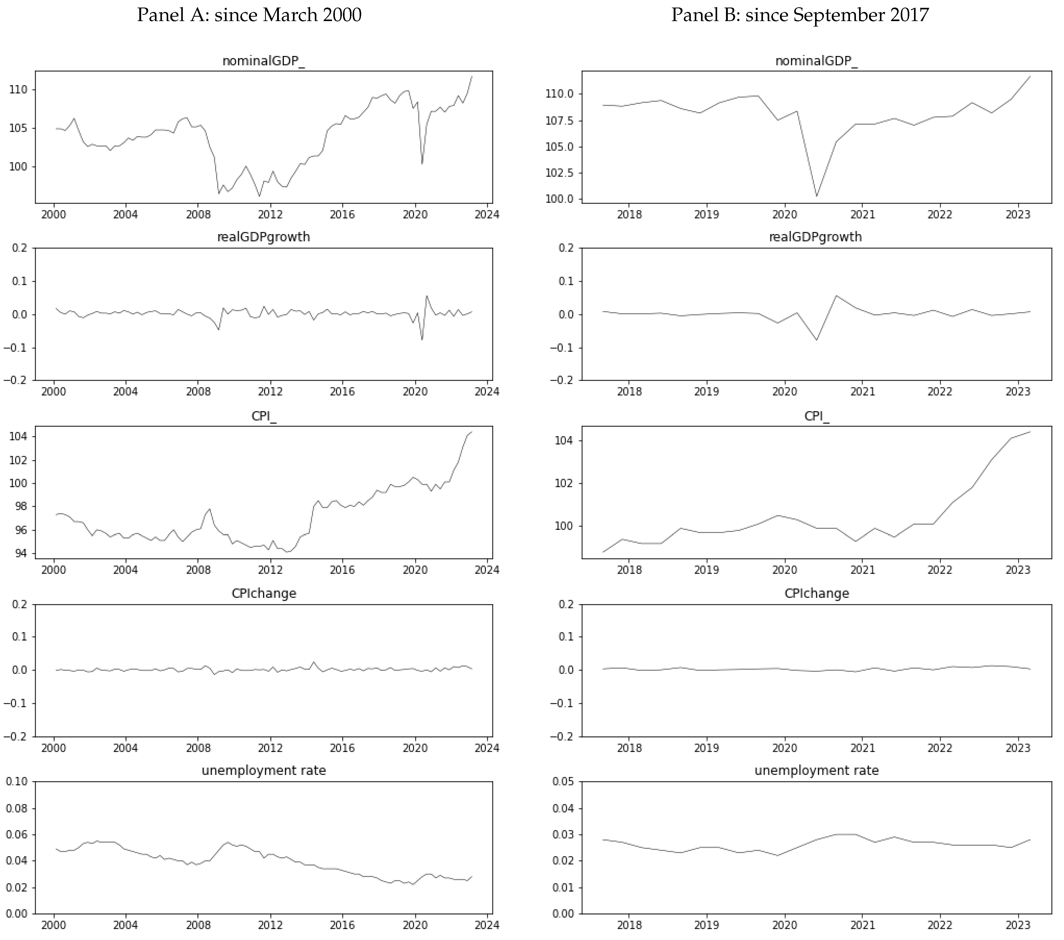
These figures can be compared with economic indicators in Japan. Panel A of Figure 4 shows the quarterly economic indicator values since 2000. Since Japan’s zero-interest-rate policy was implemented in 1999, the actual quarterly statistics for Japan from 2000 to 2022, which is considered to be a relatively similar economic environment to the current situation, have been published. We found that the nominal GDP growth rate, CPI change rate, real GDP growth rate, and unemployment rate8 are approximately 0.09% (1.38%), 0.07% (0.52%), 0.18% (1.42%), and 3.91% (0.98%), respectively. In Japan, the simulation results for the inflation rate and nominal GDP growth rate differ from the actual results due to continued deflation, but the real GDP growth rate is confirmed to be close to the simulation results. The actual unemployment rate deviates from the simulation results because Japan’s employment system, which is based on lifetime employment, keeps the actual unemployment rate low. One reason for the discrepancy in the unemployment rate could be that the model in this paper does not include firm capital goods or assets that correspond to production facilities. Because this study’s model does not include the concept of capital goods, the demand for capital goods may have been overlooked, resulting in a smaller estimate of the labor force required by firms and thus leading to a higher unemployment rate in the simulation. If the introduction of capital goods increases product demand and the number of employees, the unemployment rate may improve. However, there are numerous factors to consider, such as the industries from which to purchase capital goods and the durability of capital goods. While different from the number of bankruptcies, the closure rate reported in the White Paper on Small and Medium Enterprises in Japan shows that the closure rate in 2019 was 3.4%. The average number of bankruptcies per step in the simulation is 2.5, and one step is assumed to be one quarter, so the annualized number is 10. With 110 firm agents, the annualized bankruptcy rate is 9.1%, which is higher than the closure rate. It is conceivable that this discrepancy is derived from the minimum number of employees $y_{min}^D$ set in the simulation. Because of this minimum number of employees, there exists a lower limit to the total amount of wages paid by a firm, even in the case that the number of products sold decreases and the firm’s revenue declines. Thus, this lower limit of wage payment can possibly lead the firm to go bankrupt.

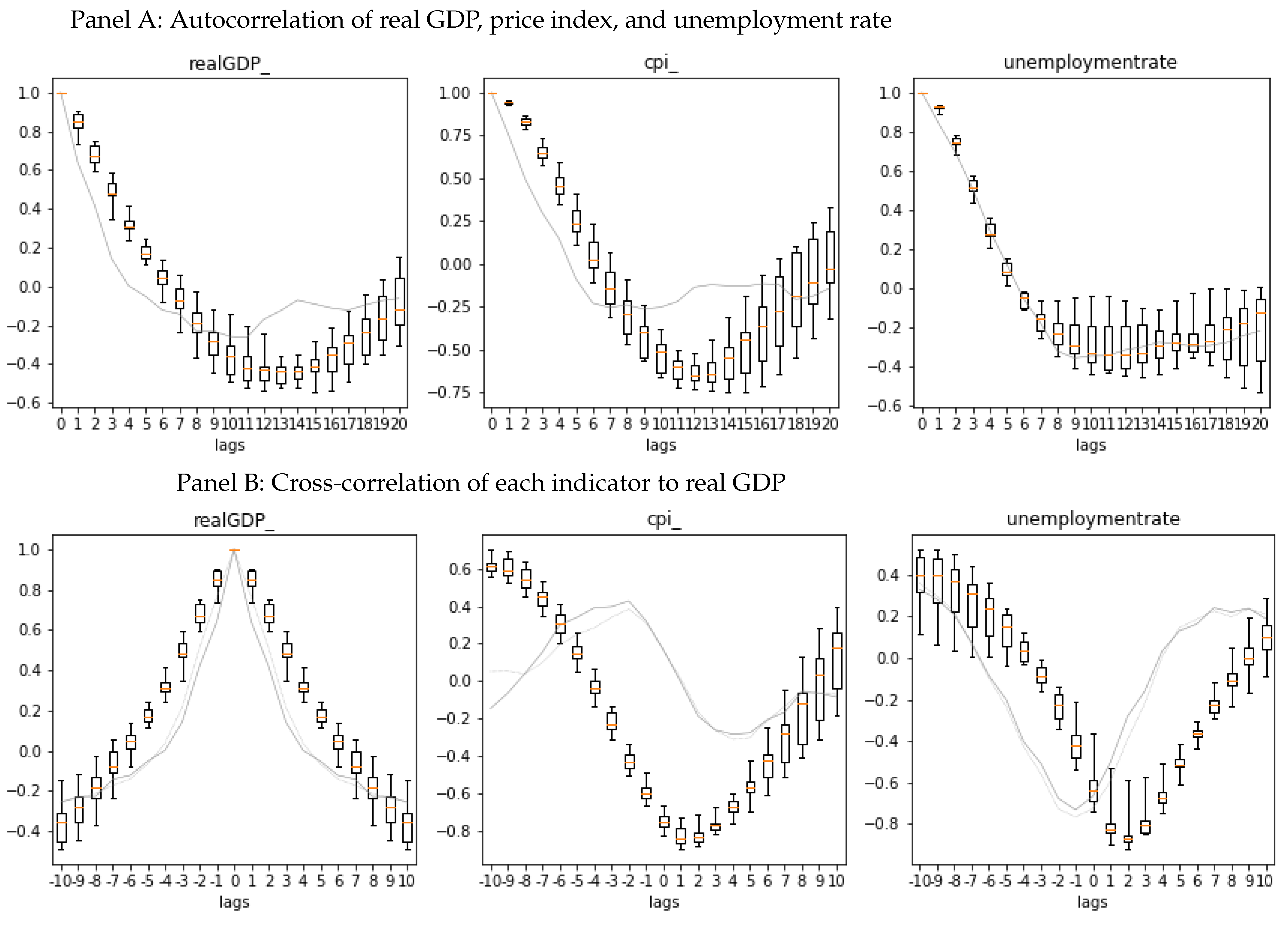
The autocorrelations and cross-correlations in the simulation results were then examined. Panel A of Figure 5 plots the autocorrelations of the real GDP, the price index, and the unemployment rate up to a lag of 20 after removing the trend component using the Hodrick–Prescott filter Hodrick and Prescott (1997). The common trend of large, positive autocorrelations during small lags and negative autocorrelations around a lag of 10 is consistent with the results of Caiani et al. (2016). Panel B shows the cross-correlation of the real GDP, price index, and unemployment rate against the real GDP after trend removal. The cross-correlations between the price index and unemployment rate to the real GDP are negative where the lags are small. Thus, the result indicating that the price index and unemployment rate decline when the real GDP rises is reasonable.

The solid gray lines in Figure 5 show the autocorrelation and cross-correlation values calculated from the actual values of economic indicators in Japan. First, the solid gray line in Panel A confirms that the behavior is consistent with the simulation results. However, we can see that the values in the simulation results tend to be more skewed than those in the simulation results. Looking at the values in Panel B, we can see that the simulation results for the price index and unemployment rate have larger amplitudes, and there are some discrepancies in the number of lags at which the maximum and minimum cross-correlation values occur. However, the results for each indicator are generally similar between those obtained from real economic indicators and those obtained from the simulation. Meanwhile, the results for each indicator can be confirmed to be generally similar to those obtained from real economic indicators and those obtained from the simulation.

5.2. Rebound of the Economy after the Resolution of Economic Shocks

As we saw in the latter half of Section 4.2, the simulation results show that, although households’ desired product consumption demand and firms’ product sales volume decreased during the economic shock, they tended to increase after the economic shock ceased to exist as compared with the case without the shock. We investigated whether such a trend exists in the real economy as well.

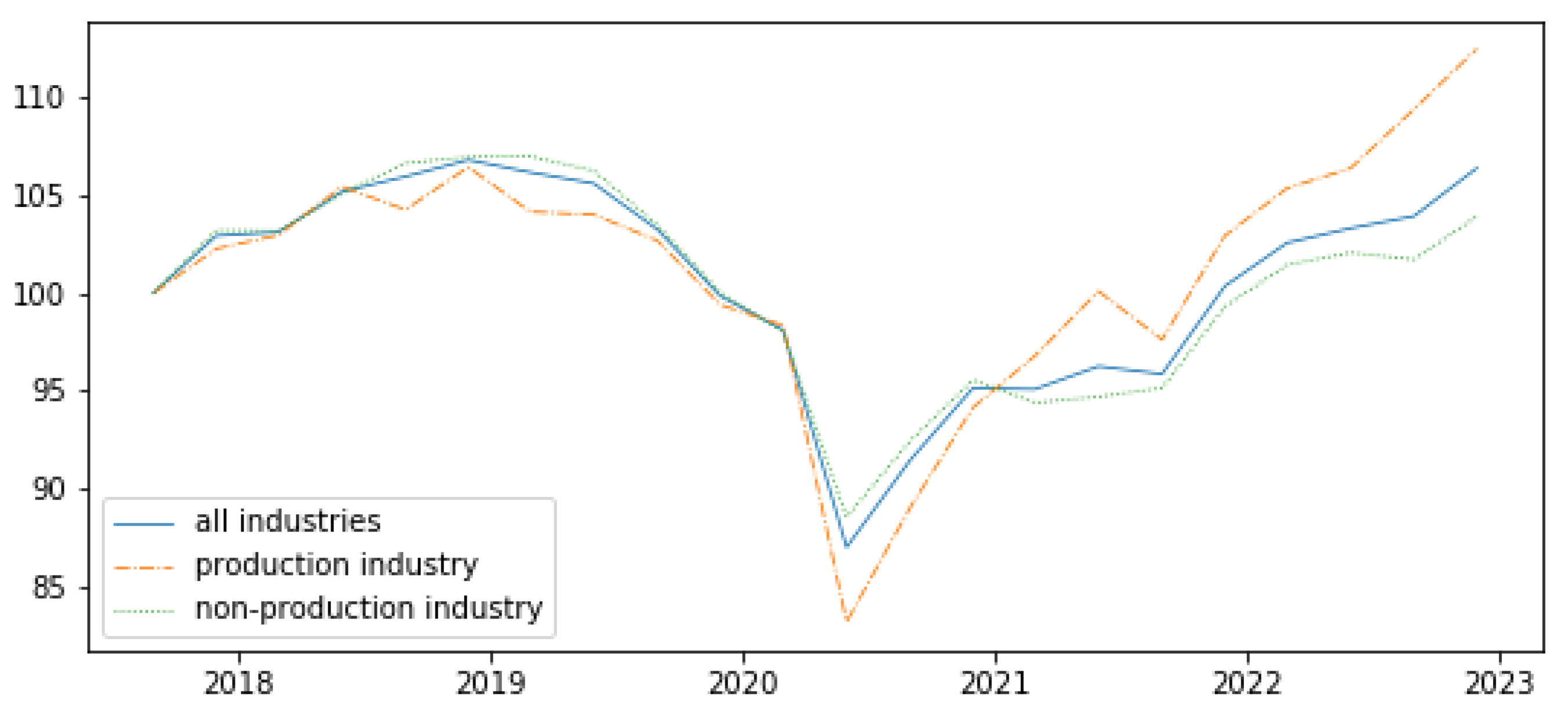
What was the change in corporate sales before and after the COVID-19 pandemic in the real Japan like? Figure 6 illustrates the transition in sales for all (blue solid line), manufacturing (orange dash-dot-dash line), and non-manufacturing (green dotted line) industries based on figures from Corporate Statistics published by Japan’s Ministry of Internal Affairs and Communications, with the value for the fourth quarter of 2019 set at 100. As shown, sales in each industry fell sharply in the first quarter of 2020 when COVID-19 spread throughout the world, and that sales in all industries increased in the fourth quarter of 2019 just before the spread. Because of the Japanese government’s cautious approach to handling coronavirus infections, Japan has lagged behind other industrialized nations in their deregulation and other efforts to prepare the situation for living with COVID-19. Even by the end of 2022, concerns about COVID-19 had not been completely dispelled. However, as previously observed, sales in the fourth quarter of 2022 rose to a level higher than that before the coronavirus shock had dissipated, implying that demand may have begun growing after the economic shock, as confirmed by simulations. With the further deregulation around coronavirus infections occurring in May 2023, the final demand is expected to recover more strongly after May 2023, and the future evolution of economic indicators will be closely monitored. However, whether the difference in the impact before and after the economic shock between the general industry and the final consumer goods industry, which was confirmed in the simulation, is consistent with the actual statistics remains unclear, given that both the manufacturing and non-manufacturing sectors include industries related to final consumer goods. We must wait for the release of more detailed economic statistics.

5.3. Avoidance of Final Consumer Goods during Economic Shocks

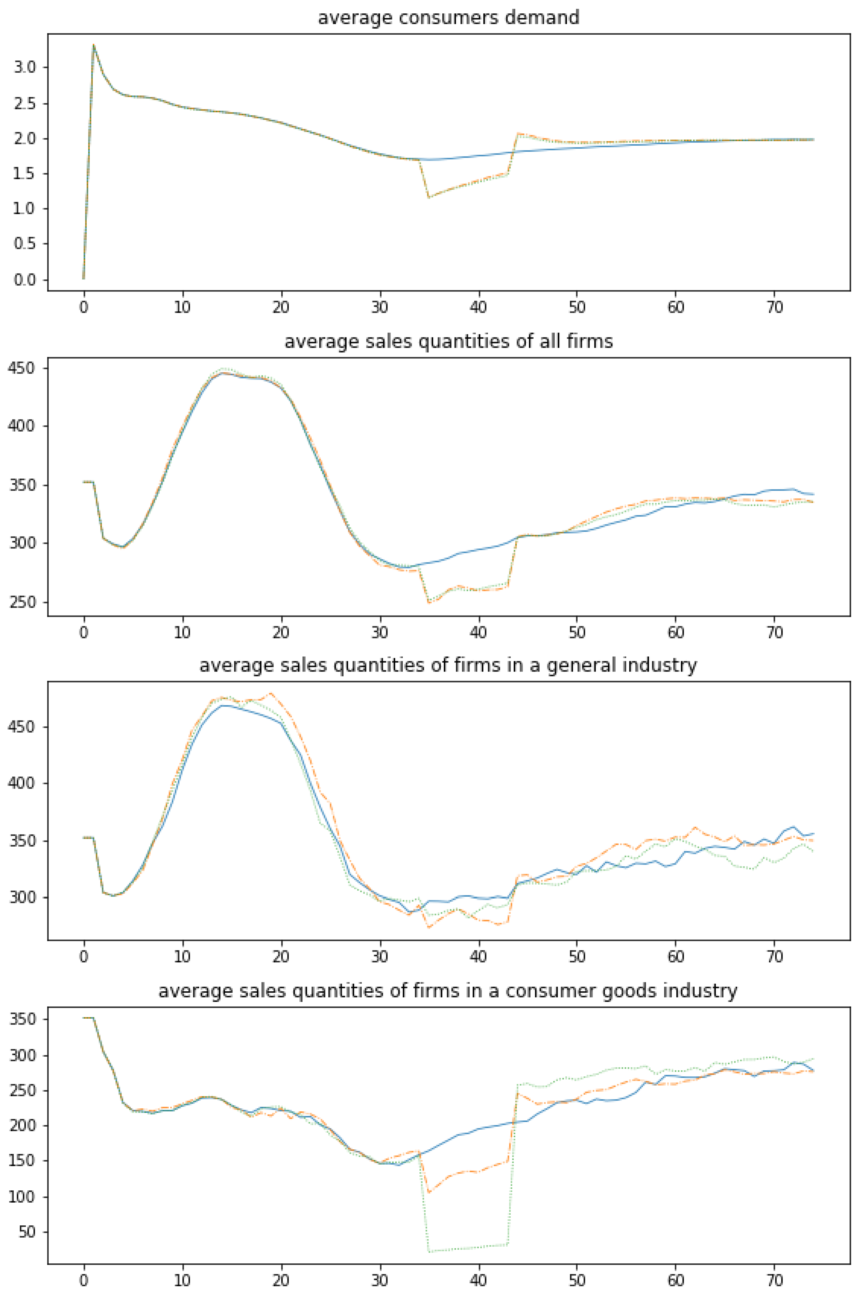
In the simulation settings, which we examined in the previous section, the selection of products by households during economic shocks was completely random. However, during an economic downturn, some industries related to final consumer goods, such as leisure and entertainment, are expected to be less likely to be selected. To reflect this situation, we implemented a mechanism in which products in the final consumption goods industry become more difficult for households to choose with a certain probability during economic shocks. The impact of economic shocks on the final consumption goods industry is expected to be relatively small for the daily necessities industry, whereas luxury-related goods such as those mentioned above are expected to be more affected. However, because the model in this paper does not distinguish between companies that provide daily necessities and companies that provide luxury goods, the mechanism is modified so that the probability of selecting the final consumer goods industry in the selection of household products is uniformly decreased. Specifically, we introduced a process that excludes final consumer goods firms from the selection target with a certain probability when households, the demand side, select the supply side in the procedure described in Algorithm 1, step 5. Figure 7 shows the changes in sales volume for the cases with an 80% probability of excluding the final consumption goods industry (green dotted line), with an economic shock but not excluding the final consumption goods industry (orange dash-dot-dash line), and without an economic shock (blue solid line).

The graph at the top in Figure 7 shows the decline in consumer demand in the event of an economic shock, and it is, of course, almost identically shaped whether or not the final consumer goods industry is excluded. The second panel shows little difference when excluding the final consumer goods industries or not when there is an economic shock, but this occurs after the end of the economic shock. The rate of increase in product sales is slower when final consumer goods industries are excluded. The third panel shows that when the final consumer goods industries are excluded, the decline in the average product sales in the general industry is smaller. When the final consumer goods industry is excluded, this is thought to be due to the stronger replacement demand from the final consumer goods industry on general industry. (In this paper, households do not prefer the industry in which manufacturing firms belong.) The fourth panel shows that when the final consumer goods industry is excluded, there is a larger decline in sales volume during the economic shock and a larger rebound after the economic shock ends.

As explained in Section 4.1, there are two industries in this paper’s model: the final consumer goods industry and general industry. The ratio of the number of firms in the general industry to those in the final consumer goods industry is 10:1, with the general industry accounting for approximately 90% of the total number of firms. The reason for the milder rebound in average sales volume after the economic shock for all firms is that the change in sales volume for the general industry, which comprises the majority, was moderate before and after the economic shock due in part to the replacement demand at the time of the economic shock.

5.4. Sensitivity Analysis

For the sensitivity analysis, we compared the base scenario of holding 2.0 months worth of intermediate input material inventories with that of 1.5 months and 1.0 month. Figure 8 shows the transitions in the nominal GDP, unemployment rate, desired production quantities, real production quantities, upper limit by labor, and upper limit by input materials. The upper limit by labor is the upper limit of the amount of product that can be produced based on the secured labor force, and the upper limit by input materials is the corresponding amount of product that can be produced based on the intermediate input material inventory. The values for the base scenario (2.0 months) are the average of 100 simulations, and the values for the cases for comparison (1.5 and 1.0) are the average of 20 simulations. Figure 8 shows that the results of the base scenario (blue solid line) and the setting of 1.5 months worth of intermediate input material inventory (green dotted line) are almost similar. This indicates that 1.5 months worth of intermediate input material inventory is sufficient enough to achieve similar results to the base scenario. On the other hand, the results of the 1.0 month inventory (orange dash-dot-dash line) show that the nominal GDP is suppressed as the simulating steps proceed while the unemployment rate remains high throughout the steps. The unemployment rate seems to have increased due to a decrease in the number of workers required as a result of sluggish product production volume. One reason for the sluggish product production volume is that the upper limit by input materials is lower than the required production quantities in later steps of the simulation, which is believed to restrain the production of products. In a case where the inventory is 1.0 month worth of intermediate input materials, there is no sufficient production capacity in a firm, and accordingly, the firm is not able to respond to the increase in demand. If intermediate goods cannot be procured as planned, the amount of products produced would have to be curtailed, and the impact of this may be transmitted to other firms through the SCN, resulting in restrained economic activity.

6. Conclusions

In this study, we attempted to incorporate the advantages of two representative approaches to build an agent-based model suitable for analyzing the propagation of shocks in an economic society. Based on a model structure that covers all major economic agents, which is one of the strengths of the macroeconomic ACE model, we constructed an agent-based model that incorporates a mechanism that links firms, such as capital goods firms and consumer goods firms, through supplier–customer relationships without establishing barriers, which is a method commonly used in corporate domain analyses.

In the simulation analysis using the proposed model, we verified the model’s validity against actual economic indicators for Japan, which fits the economic environment assumed by the model. We also confirmed that, although the actual statistics and the simulation results had some discrepancies in terms of the nominal growth rate and the unemployment rate, the simulation results were close to the statistical values of the other indicators, such as autocorrelation and cross-correlation. Subsequently, we analyzed the drop in demand and subsequent rebound in Japan during COVID-19 as an example of a shock to confirm the output of economic shocks. Although the sales volume of firms temporarily declined due to an economic shock that depressed households’ final demand, the increase in assets held by households as they refrained from consumption boosted their spending capacity. After the economic shock was resolved, firms’ sales volumes tended to be higher than before. Furthermore, we confirmed that, when the sales volume of products in the final consumer goods industry falls selectively during an economic shock, the drop in sales volume is suppressed in the general industry due to replacement demand, and the increase in the sales volume after the economic shock is milder.

The contribution of this paper is the development of a macroeconomic model that incorporates the concepts of inter-firm supplier–customer relationships and intermediate input materials. The results are generally valid for real economic data.

References

1. Brancaccio, Emiliano, Mauro Gallegati, and Raffaele Giammetti. 2021. Neoclassical influences in agent-based literature: A systematic review. Journal of Economic Surveys 36: 350–85. [Google Scholar] [CrossRef]
2. Caiani, Alessandro, Antoine Godin, and Stefano Lucarelli. 2014. Innovation and finance: A stock flow consistent analysis of great surges of development. Journal of Evolutionary Economics 24: 421–48. [Google Scholar] [CrossRef]
3. Caiani, Alessandro, Antoine Godin, Eugenio Caverzasi, Mauro Gallegati, Stephen Kinsella, and Joseph E. Stiglitz. 2016. Agent based-stock flow consistent macroeconomics: Towards a benchmark model. Journal of Economic Dynamics and Control 69: 375–408. [Google Scholar] [CrossRef] [Green Version]
4. Cincotti, Silvano, Marco Raberto, and Andrea Teglio. 2010. Credit Money and Macroeconomic Instability in the Agent-Based Model and Simulator Eurace. Available online: https://ssrn.com/abstract=1726782 (accessed on 29 April 2023).
5. Cincotti, Silvano, Marco Raberto, and Andrea Teglio. 2012. Macroprudential policies in an agent-based artificial economy. Revue de l’OFCE 124: 205–34. [Google Scholar] [CrossRef] [Green Version]
6. Copeland, Morris A. 1949. Social Accounting for Moneyflows. The Accounting Review 24: 254–64. [Google Scholar]
7. Dawid, Herbert, and Domenico Delli Gatti. 2018. Agent-Based Macroeconomics. Available online: https://ssrn.com/abstract=3112074 (accessed on 29 April 2023).
8. Dawid, Herbert, and Philipp Harting. 2012. Capturing firm behavior in agent-based models of industry evolution and macroeconomic dynamics. In Evolution, Organization and Economic Behavior. Cheltenham: Edward Elgar. [Google Scholar]
9. Deissenberg, Christophe, Sander van der Hoog, and Herbert Dawid. 2008. Eurace: A massively parallel agentbased model of the european economy. Applied Mathematics and Computation 204: 541–52. [Google Scholar] [CrossRef] [Green Version]
10. Delli Gatti, Domenico, Corrado Di Guilmi, Edoardo Gaffeo, Gianfranco Giulioni, Mauro Gallegati, and Antonio Palestrini. 2005. A new approach to business uctuations. heterogeneous interacting agents, scaling laws and financial fragility. Journal of Economic Behavior and Organization 56: 489–512. [Google Scholar] [CrossRef] [Green Version]
11. Delli Gatti, Domenico, Mauro Gallegati, Bruce Greenwald, Alberto Russo, and Joseph E. Stiglitz. 2006. Business fluctuations in a credit-network economy. Physica A: Statistical Mechanics and Its Applications 370: 68–74. [Google Scholar] [CrossRef] [Green Version]
12. Delli Gatti, Domenico, and Elisa Grugni. 2022. Breaking bad: Supply chain disruptions in a streamlined agent-based model. The European Journal of Finance 28: 1446–73. [Google Scholar] [CrossRef]
13. Delli Gatti, Domenico, and Severin Reissl. 2022. ABC: An Agent Based Exploration of the Macroeconomic Effects of COVID-19. Industrial and Corporate Change 2: 410–47. [Google Scholar] [CrossRef]
14. Di Domenico, Lorenzo, Karolina Safarzynska, and Marco Raberto. 2022. Resource Scarcity, Circular Economy and the Energy Rebound: A Macro-Evolutionary Input-Output Model. Available online: https://ssrn.com/abstract=4266965 (accessed on 22 June 2023).
15. Di Guilmi, Corrado. 2017. The agent-based approach to post Keynesian macro-modeling. Journal of Economic Surveys 31: 1183–203. [Google Scholar] [CrossRef]
16. Dilaver, Özge, Robert Calvert Jump, and Paul Levine. 2018. Agent-based macroeconomics and dynamic stochastic general equilibrium models: Where do we go from here? Journal of Economic Surveys 32: 1134–59. [Google Scholar] [CrossRef]
17. Dosi, Giovanni, Giorgio Fagiolo, and Andrea Roventini. 2006. An evolutionary model of endogenous business cycles. Computational Economics 27: 3–34. [Google Scholar] [CrossRef] [Green Version]
18. Dosi, Giovanni, Giorgio Fagiolo, and Andrea Roventini. 2008. The microfoundations of business cycles: An evolutionary multi-agent model. Journal of Evolutionary Economics 18: 413–32. [Google Scholar] [CrossRef]
19. Dosi, Giovanni, Giorgio Fagiolo, and Andrea Roventini. 2010. Schumpeter meeting Keynes: A policy-friendly model of endogenous growth and business cycle. Journal of Economic Dynamics and Control 34: 1748–67. [Google Scholar] [CrossRef] [Green Version]
20. Dosi, Giovanni, Marcelo C. Pereira, Andrea Roventini, and Maria Enrica Virgillito. 2022. Technological paradigms, labour creation and destruction in a multi-sector agent-based model. Research Policy 51: 104565. [Google Scholar] [CrossRef]
21. Fujiwara, Yoshi, and Hideaki Aoyama. 2008. Large-scale structure of a nation-wide production network. The European Physical Journal B 77: 565–80. [Google Scholar] [CrossRef]
22. Godley, Wynne, and Marc Lavoie. 2007. Monetary Economics An Integrated Approach to Credit, Money, Income, Production and Wealth. New York: Palgrave MacMillan. [Google Scholar]
23. Guan, Dabo, Daoping Wang, Stephane Hallegatte, Steven J. Davis, Jingwen Huo, Shuping Li, Yangchun Bai, Tianyang Lei, Qianyu Xue, D’Maris Coffman, and et al. 2020. Global supply-chain effects of COVID-19 control measures. Nature Human Behaviour 4: 577–87. [Google Scholar] [CrossRef]
24. Haldane, Andrew, and Arthur Turrell. 2018. An interdisciplinary model for macroeconomics. Oxford Review of Economic Policy 34: 219–51. [Google Scholar] [CrossRef]
25. Hillman, Robert, Sebastian Barnes, George Wharf, and Duncan MacDonald. 2021. A New Firm-Level Model of Corporate Sector Interactions and Fragility: The Corporate Agent-Based (CAB) Model. OECD Economics Department Working Papers 1675. Paris: OECD. [Google Scholar]
26. Hodrick, Robert J., and Edward C. Prescott. 1997. Postwar U.S. Business Cycles: An Empirical Investigation. Journal of Money, Credit and Banking 21: 1–16. [Google Scholar] [CrossRef]
27. Inoue, Hiroyasu. 2021. Propagation of International Supply-Chain Disruptions between Firms in a Country. Journal of Risk and Financial Management 14: 461. [Google Scholar] [CrossRef]
28. Inoue, Hiroyasu, and Yasuyuki Todo. 2019. Firm-level propagation of shocks through supply-chain networks. Nature Sustainability 2: 841–47. [Google Scholar] [CrossRef]
29. Inoue, Hiroyasu, and Yasuyuki Todo. 2020. The propagation of economic impacts through supply chains: The case of a mega-city lockdown to prevent the spread of COVID-19. PLoS ONE 15: e0239251. [Google Scholar] [CrossRef] [PubMed]
30. Kinsella, Stephen. Words to the Wise: Stock Flow Consistent Modeling of Financial Instability. Available online: https://ssrn.com/abstract=1955613 (accessed on 29 April 2023).
31. Newman, Mark E. J. 2005. Power laws, Pareto distributions and Zipf’s law. Contemporary Physics 5: 323–51. [Google Scholar] [CrossRef] [Green Version]
32. Ohno, Takashi, and Hiroshi Nishi. 2011. Reconstructing Kaleckian Model: Stock-Flow Consistent Model. Political Economy Quarterly 47: 6–18. (In Japanese). [Google Scholar]
33. Otto, Christian, Sven N. Willner, Leonie Wenz, and Katja Frieler. 2017. Modeling loss-propagation in the global supply network: The dynamic agent-based model acclimate. Journal of Economic Dynamics and Control 83: 232–69. [Google Scholar] [CrossRef] [Green Version]
34. Perera, Supun, Michael G. H. Bell, and Michiel C. J. Bliemer. 2017. Network science approach to modelling the topology and robustness of supply chain networks: A review and perspective. Applied Network Science 2: 33. [Google Scholar] [CrossRef] [Green Version]
35. Pichler, Anton, Marco Pangallo, R. Maria del Rio-Chanona, François Lafond, and J. Doyne Farmer. 2020. Production Networks and Epidemic Spreading: How to Restart the UK Economy? Available online: https://ssrn.com/abstract=3606984 (accessed on 7 July 2023).
36. Poledna, Sebastian, Michael Gregor Miess, Cars Hommes, and Katrin Rabitsch. 2023. Economic forecasting with an agent-based model. European Economic Review 151: 104306. [Google Scholar] [CrossRef]
37. Rahman, Towfique, Firouzeh Taghikhah, Sanjoy Kumar Paul, Nagesh Shukla, and Renu Agarwal. 2021. An agent-based model for supply chain recovery in the wake of the COVID-19 pandemic. Computers and Industrial Engineering 158: 107401. [Google Scholar] [CrossRef]
38. Reissl, Severin, Alessandro Caiani, Francesco Lamperti, Mattia Guerini, Fabio Vanni, Giorgio Fagiolo, Tommaso Ferraresi, Leonardo Ghezzi, Mauro Napoletano, and Andrea Roventini. 2022. Assessing the Economic Impact of Lockdowns in Italy: A Computational Input–Output Approach. Industrial and Corporate Change 31: 358–409. [Google Scholar] [CrossRef]
39. van der Hoog, Sander, and Herbert Dawid. 2015. Bubbles, Crashes and the Financial Cycle Insights from a Stock-Flow Consistent Agent-Based Macroeconomic Model. Available online: https://ssrn.com/abstract=2616662 (accessed on 29 April 2023).
Figure 1. Transitions of main economic indices in each of the 100 trials. Each line shows the results of each simulation. (Panel A) shows the results up to 400 steps while (Panel B) shows up to 100 steps.
Risks 11 00128 g001
Figure 2. Transitions in average product sales quantities of the firms grouped by number of customers or suppliers. The first column shows the average product sales volume of the firms grouped by the number of customers and the second column is grouped by the number of suppliers.
Risks 11 00128 g002
Figure 3. Transitions in consumption demand and product sales volume before and after an economic shock. The blue solid line shows the result without an economic shock, the green dotted line shows the result with a short-term shock at step 35, and the orange dash-dot-dash line shows the result with a long-term shock from the 35th to the 43rd steps. The first row shows the transition in final demand, the second row shows average sales volume for all firms, the third row shows average sales volume for firms in a general industry, and the fourth row shows average sales volume for firms in the consumer goods industry.
Risks 11 00128 g003
Figure 4. Transitions in economical indicators. (Panel A) shows the transitions since March 2000, while (panel B) shows transitions since September 2017.
Risks 11 00128 g004
Figure 5. Autocorrelation of key indicators and cross-correlation of key indicators to real GDP. Cyclical elements are subject to analysis, while trend elements are removed by the HP filter. Autocorrelations are estimated up to a lag of 20. Cross-correlations are estimated from 10 leads to 10 lags. A −10 lag indicates 10 leads in each graph in (panel B). The solid gray lines show the autocorrelation and cross-correlation values calculated from the actual values of economic indicators in Japan.
Risks 11 00128 g005
Figure 6. Corporate sales in Japan before and after the coronavirus shock based on figures from Corporate Statistics published by Japan’s Ministry of Internal Affairs and Communications, with the value of the last quarter of 2019 set at 100.
Risks 11 00128 g006
Figure 7. The blue solid line shows the result without economic shock, the green dotted line shows the result with a long-term shock from the 35th to the 43rd steps and restricted choice of final consumer goods, and the orange dash-dot-dash line shows the result with a long-term shock from the 35th to the 43rd steps and no restricted choice (the same with the orange dash-dot-dash line in Figure 3). The first row shows the transition in final demand, the second row shows average sales volume for all firms, the third row shows average sales volume for firms in a general industry, and the fourth row shows average sales volume for firms in the consumer goods industry.
Risks 11 00128 g007
Figure 8. Transitions in average of nominal GDP, unemployment rate, desired production quantities, real production quantities, upper limit by labor, and upper limit by input materials. The blue solid line shows the result with input material inventory sufficient to cover two months, the green dotted line with 1.5 months worth of input material inventory, and the orange dash-dot-dash line with 1.0 month worth of input material inventory.
Risks 11 00128 g008