Article

Underwriting Cycles in Property-Casualty Insurance: The Impact of Catastrophic Events

by
Annette Hofmann
1,* and
Cristina Sattarhoff
2,3
1
Carl H. Lindner College of Business, University of Cincinnati, Cincinnati, OH 45221, USA
2
Department of Economics, University of Kiel, Wilhelm-Seelig-Platz 1, 24118 Kiel, Germany
3
Faculty of Business Administration, HBS Hamburg Business School, University of Hamburg, Moorweidenstraße 18, 20148 Hamburg, Germany
*
Author to whom correspondence should be addressed.
Risks 2023, 11(4), 75; https://doi.org/10.3390/risks11040075
Submission received: 27 February 2023 / Revised: 27 March 2023 / Accepted: 29 March 2023 / Published: 11 April 2023
(This article belongs to the Special Issue Risks: Feature Papers 2023)

Abstract

:
This paper challenges the question of existence and predictability of underwriting cycles in the U.S. property and casualty insurance industry. Using an approach in the frequency domain, we demonstrate the existence of a hidden periodic component in annual aggregated loss ratios. The data support an underwriting cycle length of 8–9 years. Going beyond previous research and studying almost 30 years of quarterly underwriting data, we can improve forecasting performance by (dis)connecting cycles and catastrophic events. Superior out-of-sample forecast results from models with intervention variables flagging the time point of catastrophic outbreaks is achieved in terms of mean squared/absolute forecast errors. We evaluate model confidence sets containing the most accurate model with a certain confidence level. The analysis suggests that reliable forecasts can be achieved net of the irregular major peaks in loss distributions that arise from natural catastrophes as well as unusual “black swan” events.

1. Introduction

The dynamics of underwriting profits in the property and casualty insurance industry have been subject to various studies. It is often argued that these profits tend to exhibit a clear pattern of cyclical recurrence. An underwriting cycle is defined as the tendency of property and casualty insurance premiums, profits, and available coverage to exhibit a cyclical pattern over time. These cycles have traditionally been viewed as dynamically shifting back and forth between hard and soft market phases (Harrington et al. 2013). In a soft market phase, insurers tend to expand their market share through cutting prices and by offering generous coverage. A soft market phase is thus characterized by readily available insurance and relatively low underwriting profits. In contrast, in a hard market phase, insurers raise their premiums, thereby limiting coverage availability, and consequently enhancing their underwriting profits. Stricter underwriting standards and higher prices imply higher profits and accumulation of capital. The expansion of underwriting capacity increases competition, which decreases prices and then relaxes underwriting standards. The lowering of standards may imply more potential underwriting losses, which sets the stage for a new cycle to begin. The underwriting cycle phenomenon is similar to general business cycles in the aggregate economic activity, as well as to financial bull and bear markets when evaluating stock price dynamics.1 Likewise, insurance practitioners recognize the cycle phase as an industry fact.2 Yet, the interesting question is to what extent they can (and should) use this information. Can it be used to improve their pricing methods or selling budgets in order to increase profits? Underwriting cycles are often thought to be unpredictable in nature and, hence, represent a major challenge for the insurance industry. This study challenges this often-cited “unpredictability” argument.
Boyer et al. (2012) employ annual loss ratios for the property and casualty industry during the period of 1967–2004. Nine models are analysed: two models with deterministic trend, six business cycle models, and an autoregressive model, which is also the benchmark model. They report similar predictive power for the business cycle models and the benchmark model in their study. Given that one would expect superior forecasting results for the more elaborated business cycle models if it were indeed the case that cycles really existed in the underwriting data, the authors interpret their findings as evidence of unpredictability in general by stating that “our results imply that it is impossible to reliably forecast loss ratios for the property and casualty insurance industry using only their past values” (Boyer et al. 2012, p. 1008). Revisiting this statement leads us to find this was an exaggeration. Our study challenges previous studies with similar findings by arguing that former research used limited data and/or that the models under consideration had limited predictive accuracy. Nevertheless, the most interesting and important message of Boyer et al. (2012) is that business cycle models are inappropriate as such for modeling and forecasting loss ratio data.3
The most prevalent time series method for the analysis and calculation of underwriting cycles is the autoregressive model. Mostly, a second order model is employed, some authors adding additional exogenous variables, e.g., trend, money market rate, yield on 5-year US Treasury Bonds, reinsurance price index, or controlling for the influence of catastrophic events (Cummins and Outreville 1987; Harrington et al. 2013; Meier and Outreville 2006). Occasionally, periodograms and spectrum estimates were used for calculating cycle lengths (Grace and Hotchkiss 1995; Meier 2006). More recently, modern techniques also emerged: business cycle models (Boyer et al. 2012), error correction models for the cointegrating relationship between loss ratios and macroeconomic variables (Jawadi et al. 2009) or between losses and premiums (Lazar and Denuit 2012), regime-switching Markov models (Wang et al. 2011), agent-based models (Owadally et al. 2018, 2019a), and data mining techniques borrowed from data science (Owadally et al. 2019b).
In this paper, we recalculate the underwriting cycle length using a testing procedure in the frequency domain based on the maximum periodogram ordinate going back to Fisher (1929), the so-called Fisher’s G-test. This can be used to detect hidden periodicities. Several extensions (Ahdesmäki et al. 2005; Bartlett 1957; Bølviken 1983; Chiu 1989; Hannan 1961; Siegel 1980; Whittle 1952) and numerous applications in seismology, astronomy, oceanography, acoustics, and medicine (Ahdesmäki et al. 2005; Hohensinn et al. 2020; Telesca et al. 2015) are available. By contrast, economic applications are scarce; we mention here Canova (1996) for the analysis of business cycles and Yilmaz et al. (2018) for production cycles.
One of the reasons for the scarcity of spectral analyses in econometrics in general and for the study of underwriting cycles in particular is the absence of a model to explain the rationale of cycles. Additionally, authors’ negligence in providing significance levels for spectral analysis results has contributed to a general skepticism in the context of insurance cycle research about the reliability of these methods (Venezian 2006; Venezian and Leng 2006).
This study employs an updated version of Fisher’s G-test which is a theoretically well-founded method. Fisher (1929) employed the distributional characteristics of the periodogram under the Gaussian assumption to derive exact p-values for a realization of the G-statistic. In applications, large datasets are required for the calculation of reliable empirical approximations. Ahdesmäki et al. (2005) introduced a robust version of Fisher’s G-test which is applicable for short time series, being also insensitive to a large range of alternative anomalies (e.g., outliers, missing values, non-Gaussian noise).
It seems less of a question whether underwriting cycles are real—a simple look at the series in Figure 1 confirms the presence of a dominant cyclical pattern. In Section 3, we test on the presence of a hidden periodic component in the annual loss ratio data and find evidence in favour of this. The question is rather whether reliable predictions can be made based on this cyclical pattern and by using available information for forecasting. Thus, the main focus of this study is to demonstrate that it is indeed possible to increase forecasting accuracy by using an additional source of information: information on catastrophic events or major ’peaks’ in the underwriting data.
Note that, following the evolution of loss ratios in Figure 1, catastrophes play a “triggering role” by inducing the downward movement in cycles. As a result, we find superior forecasting performance in models with intervention variables for catastrophes, as compared to models not considering catastrophic events. Our analysis builds on the idea of (dis)connecting cycles and catastrophic events—which seems intuitive since many catastrophes are unsystematic and rare events following autonomous dynamics. As a consequence, going beyond previous studies, we suggest that reliable forecasts can be performed through the combination of the irregular peaks in loss distributions arising from natural and other catastrophes, as well as unusual “black swan” events.
From an economic point of view, cyclicality seems to be an intrinsic property of insurance underwriting performance. Visual inspection of underwriting data shows that loss ratio series typically fluctuate within a specific confidence band. They do not depart from that band, nor do they wander away like financial asset prices, but are characterized by somewhat regular ups and downs. This relates to the management of insurance companies and state regulations which can prevent companies from declaring bankruptcy, even in the case of a major catastrophic event, such as 9/11. In the case of a catastrophic event, the insurance company will redistribute risks and costs so as to push loss ratios down again.4 This business mechanism explains why peaks in the data, i.e., catastrophes and other large loss events, typically mark the onset of the downward movement in a particular cycle.
The contribution of this paper is threefold: First, based on a robust version of Fisher’s G-test, we confirm the existence of underwriting cycles with a length of 8 to 9 years for the aggregated annual loss ratio data for the U.S. Our result is in line with cycle lengths reported elsewhere in the literature for the U.S. property and casualty insurance industry: see, for example, Owadally et al. (2019b), who employ a data science algorithm for the discovery of periodicities, the so-called motif-based periodicity detection scheme, Lazar and Denuit (2012) who analyse the dynamic relationship between premiums and losses with a vector error correction model, Meier and Outreville (2006) who study the reinsurance price index and confirm a highly cyclical pattern with a calculated cycle length of approximately 9 years, having a significant influence on the primary market’s loss ratios, and Grace and Hotchkiss (1995) using a spectrum estimate for quarterly combined ratio data. It is important to note that the methodology proposed in this paper is straightforward and easily to implement. The robust G-test is a very promising tool, all the more considering that this is the first application to underwriting cycles.
Second, in this paper, we use the information on catastrophes to increase forecasting performance. The basic scenario employs linear autoregressive models with additional dummy variables marking catastrophic outbreaks.5 In Section 4, we introduce more elaborate intervention variables which can model the catastrophic event effect more precisely. It is then also possible to evaluate this effect, i.e., we can separate between normal fluctuations and fluctuations attributable to a catastrophic event.
Finally, the current study uses a new and much larger set of quarterly loss ratio observations as compared to previous studies.
The paper is structured as follows. The next section reviews previous research. Section 3 evaluates periodicities in annual underwriting data and tests for an unknown periodicity in these data. Section 4 discusses methodological issues regarding intervention models and their estimation procedure. We describe our quarterly data for individual companies in Section 5 followed by two empirical applications: Section 6 evaluates the impact of catastrophic events. Section 7 computes loss ratio forecasts and backtests to check the predictive performance of our models on historical data using a rolling window scheme. The last section concludes.

2. Previous Research

Various hypotheses have been developed to explain underwriting cycles in the property/casualty insurance market: (1) financial pricing hypothesis, (2) capacity constraints hypothesis, (3) financial quality hypothesis, and (4) option pricing approach.
(1) Financial pricing hypothesis: This hypothesis indicates that insurance premiums reflect the discounted value of costs associated with losses. Assuming prices to be driven by competition in a competitive insurance market, only temporary (but not long-term) deviations from an assumed market equilibrium could be explained by random changes in demand and supply. It is therefore interesting to examine the drivers of the large cycles visible in this industry. Cummins and Outreville (1987) study the financial pricing hypothesis by attributing such cyclical pattern to a second-order autoregressive process that includes insurance information, regulatory, and reporting lags. Studying the same hypothesis, subsequent studies by Doherty and Kang (1988) and Lamm-Tennant and Weiss (1997) also find consistent results.6 However, in these studies it is implicitly assumed that insurers act in a risk-neutral way and that markets are perfect.7
(2) Capacity constraints hypothesis: This hypothesis assumes that the capital market is not perfect in the sense that shocks to capital—by events such as, e.g., large catastrophic losses—result in cycles. Capital cannot move immediately and without cost into and out of the insurance market, creating capacity constraints. To date, there have been numerous articles focusing on this theory, including Winter (1988, 1994), Niehaus and Terry (1993), Gron (1994a), as well as Gron (1994b), Doherty and Garven (1995), and Doherty and Posey (1997). However, while underwriting profits are inversely dependent on capacity in the short term, profits do not depend on capacity in the long term. As argued by Winter (1994), and Gron (1994a, 1994b), asymmetric information availability in the insurance market prevents insurers from quickly adjusting their capacity to maintain a long-term equilibrium. Hence, a negative capital shock may rapidly increase premiums along with underwriting profits. The existence of this relationship is tested by examining whether capacity is negatively related to underwriting profits.
(3) Financial quality hypothesis: This hypothesis assumes that insurance company’s premiums endogenously depend on its insolvency potential. Harrington and Danzon (1994) and Cagle and Harrington (1996) study insurer financial quality in the sense of endogenous insolvency risk in insurance prices. The financial quality hypothesis has the same short term implications as the capacity constraints hypothesis. By contrast, the financial quality hypothesis maintains that long-term underwriting profits should depend positively on capacity levels, since higher levels of financial quality lead to consumers presumably willing to pay more for higher quality policies.
(4) Option pricing approach: This hypothesis assumes policyholders to have a short position in a put option on insurer assets. This put option is referred to as the insolvency put. An insurer’s insolvency risk, and hence the value of the option, increases when insurer capacity goes down. In other words, an insurer’s underwriting profits increase with its capacity in both the short and long term. The option pricing approach is studied by Cummins and Sommer (1996).
Arguing that all above hypotheses assume insurer risk neutrality (instead of the more realistic risk-averse behaviour of firms) and that a competent study needs to simultaneously assess both the long term and short term effects, Jiang and Nieh (2012) use U.S. insurance underwriting profits from 1950 to 2009 to show that the financial pricing hypothesis may be the most suitable model for explaining historical insurance pricing patterns. The authors can explain the cyclical pattern in underwriting profits as a dynamic feedback to the long-term market equilibrium. These competition-originated cycles are analysed by Malinovskii (2010), who shows, theoretically, that aggressive low-price market intrusion by a new competitor may trigger a concerted industry response—which implies premiums being slashed and some competitors going into insolvency. Boonen et al. (2018) model the potential existence of premium cycles in competitive insurance market equilibrium. Their first framework assumes an exponential relation between premium strategies and business volume. The second is a two-step model first characterizing competition between any selected pair of insurers and then aggregating all the paired competitions in the market. It is shown numerically that indeed premium cycles may result in equilibrium.8
Meier and Outreville (2006) study the existence of underwriting cycles in the property/liability insurance industry for France, Germany, and Switzerland and the European reinsurance industry. Loss ratio data are examined for 1982 to 2001 in connection with the reinsurance and the money market rates. A major finding is that the reinsurance price index tends to be highly cyclical with a calculated cycle length of approximately nine years, having a significant influence on the primary market’s loss ratios.
Browne et al. (2014) use data from the U.S. property and casualty insurance industry to show that insurers who pay contingent commissions—that is, payments to their brokers based on the volume and profitability of business placed—experience fewer price fluctuations over the underwriting cycle than insurers who do not pay contingent commissions. Lei and Browne (2017) show that (i) product concentration, (ii) geographic concentration, and (iii) focus on states with caps on general damages display trends that run opposite of the combined ratio in medical malpractice insurance. During soft markets, insurers employ a looser underwriting strategy with lower product and geographic concentration, and less focus on safer states; during hard markets, underwriting is more difficult, reduced capacity implies that insurers write less policies, and prices are high (Marx (2013)). Confirming the capital constraints hypothesis, empirical results show that weakened capital bases at the firm level are associated with tighter underwriting.
At the end of the day, there is little consensus with respect to which hypothesis best explains the pricing patterns and “no single hypothesis can explain thoroughly the insurance cycle” (Browne et al. 2014, p. 2378). The usual approach to study underwriting cycles in the insurance literature is the autoregressive (AR) model. Using AR model estimates, a large body of literature evaluates whether there is evidence of cycles in annual U.S. insurance underwriting performance as measured by premium-to-loss or simply loss ratio time series. Following Fung et al. (1998), Guo et al. (2009), and Lazar and Denuit (2012), Boyer et al. (2012) question the existence of underwriting cycles in the property and casualty insurance industry. The authors use (only) 38 annual observations to show that AR models estimates are not consistent with evidence for cyclicality and that usage of different filters from the business cycle literature cannot improve forecasting capabilities.
In general, forecasts reliability is subject to three types of uncertainty: (1) uncertainty about the selected model, (2) uncertainty about the estimated model parameters, and (3) uncertainty about future shocks (Chatfield 1993). Here, a clear distinction must be drawn between cross-sectional analysis (where one can assume independent model errors) and longitudinal analysis based on time series data (here the error term is typically autocorrelated). In the latter case, particularly large time series are required to ensure reliability of model estimates. We note that previous research on underwriting cycles typically used small data samples with an average length of 30 observations. Inspired by Boyer et al. (2012), the current study uses much longer time series and a different modeling approach in order to further evaluate the question of existence and predictability of underwriting cycles in the property/casualty insurance industry.

3. Are Underwriting Cycles Real?

Figure 1 displays the annual aggregated loss ratios for the period 1967–2018 (52 observations) in the U.S. property and casualty insurance industry.9 Loss ratios are a useful tool in the insurance industry to represent the relationship between losses and earned premiums. Losses in loss ratios not only include paid insurance claims, but also adjustment expenses.
The periodogram analysis is a useful method to reveal periodicities in time series. In the following, we will use techniques based on the periodogram analysis to detect and approximate potential cyclic patterns. Figure 2 (left section) displays a smoothed spectral estimate for the detrended annual loss ratios. The distribution of the spectral estimator was approximated by a χ 2 distribution using the Satterthwaite approximation and confidence intervals were calculated. The dominant peak at frequency 0.12 would suggest a periodic component with length of approximately 8.5 years.
In particular, this section is devoted to a test for an unknown periodicity in the annual data going back to Fisher (1929).10 Most recently, extensions were proposed by Siegel (1980), Bølviken (1983) and Ahdesmäki et al. (2005) proving higher power compared with Fisher’s test when multiple periodic components are present in the data and in the case of periodic components with non-Fourier frequencies (McSweeney 2006). Artis et al. (2004) compare between six major groups of methods for the estimation of hidden periodicities including mixed spectrum methods and Pisarenko’s harmonic decomposition method (Kay and Marple 1981; Pisarenko 1973). The authors also consider two enhancements to Fisher’s test introduced by Chiu (1989) and report good power properties for the latter via extensive simulation studies.
In this paper we use a robust version of Fisher’s test introduced in Ahdesmäki et al. (2005) which is applicable for short time series, being also insensitive to a large range of alternative anomalies (e.g., outliers, missing values, non-Gaussian noise). Ahdesmäki et al. (2005) follow the original approach by Fisher (1929) who considers the following model with a harmonic wave of frequency λ :
Y t = a cos 2 π λ t + b sin 2 π λ t + ε t ,
with ε t Gaussian white noise, ε t i . i . d . N 0 , σ 2 . Here, Y t models loss ratios after having eliminated the trend whereas the frequency λ is unknown, 0 < λ < 0.5 . Parameters a and b determine the height (or amplitude) of the cycle and its phase, i.e., the location of the first peak. (See also Appendix A for supplementary regression diagnostics.) Our aim is to test the hypotheses
H 0 : a = b = 0 vs . H 1 : a 0 b 0 .
If the null hypothesis is false, there is a harmonic wave capturing the inherent cycle in the observed loss ratio data. In this case, the periodogram would have a large value at one point and small values of similar magnitude otherwise. Fisher’s test statistic G exploits exactly this property for the (scaled) periodogram J λ ,
J λ = N 1 N t = 1 N y t cos 2 π λ t 2 + 1 N t = 1 N y t sin 2 π λ t 2 .
Under the null hypothesis, Y t is Gaussian white noise, Y t i . i . d . N 0 , σ 2 . Then, the following applies for the normalized periodogram ordinates:
2 J ( λ k ) σ 2 i . i . d . χ 2 2
when evaluated at the Fourier frequencies
λ k = k N , k = 1 , , M = N 1 2 .
Here, N denotes the total number of observations. By contrast, if the model Y t contains a hidden periodicity, then the periodogram should have a peak in the interval 0 , 0.5 . Thus, Fisher (1929) uses the maximum periodogram ordinate max 1 k M J λ k and tests whether this ordinate can be considered as the maximum in a random sample of M i.i.d. χ 2 2 distributed random variables. Figure 2 (right section) displays the periodogram for the annual loss ratios after having eliminated a quadratic trend from the data. As a matter of fact one can see a dominant peak at frequency λ = 0.1154 .
Fisher’s test statistic is given by
G = max 1 k M J λ k 1 M k = 1 M J λ k with P ( T t ) = 1 1 e t M H 0
where the denominator is the noise variance estimator σ ^ 2 = 1 M k = 1 M J λ k . The test procedure is as follows:
1.
Calculate the value of the test statistic G * .
2.
Determine the critical value κ α at significance level α 0 , 1 :
κ α = ln 1 1 α 1 / M
or, alternatively, the p-value
P ( G G * ) = 1 1 e G * M .
3.
Reject H 0 at significance level α if
G * > κ α or , alternatively , P ( G G * ) < α .
Ahdesmäki et al. (2005) replace the periodogram J ( λ k ) in (2) by a robust (indirect) smoothed spectral estimator which evaluates the correlations in the data. Their statistic no longer obeys the closed form distribution depicted above according to Fisher (1929). p-values can be computed based on an empirical approximation of the distribution function using Monte Carlo simulations. According to this the Gaussian assumption becomes obsolete.11
We obtain the p-value of 8 × 10 5 for the robust test of Ahdesmäki et al. (2005). Thus, we can reject the null hypothesis in favour of a hidden periodicity (significance level 5%). It is noteworthy that this result suggests the presence of a cyclical pattern in the U.S. annual loss ratio data. The unknown frequency for the hidden periodic component can be approximated by the frequency λ = 0.1154 corresponding to the peak in the periodogram, i.e., the data support a (hidden) cycle length of approximately 8 to 9 years. This result is consistent with Owadally et al. (2019b), who employ a data science algorithm for the discovery of periodicities, the so-called motif-based periodicity detection scheme (reported cycle length 8.5 years) and Lazar and Denuit (2012) who analyse the dynamic relationship between premiums and losses with a vector error correction model (reported cycle length of approximately 8 years). Alternatively, the latter study also evaluates smoothed spectrum estimates (reported cycle length of approximately 8.5 years). Similarly, Grace and Hotchkiss (1995) use quarterly aggregated combined ratio data for the U.S. during 1974–1990. Based on spectral estimation they report a cycle length of 8.4 years. (Additionally, they also detect an annual periodicity of seasonal character due to the quarterly frequency of their data.) Appendix A reports additional diagnostics for the harmonic regression (1).

4. An Intervention Model for Quarterly Underwriting Data

This paper demonstrates a possibility to increase predictive accuracy when using models that differentiate between two sources of information: information on the cycles and information on the catastrophic events. For this purpose, we use quarterly loss ratio data for four insurance companies. This allows for a more accurate evaluation of catastrophes than has been possible before. In Section 7, following the forecast design in Boyer et al. (2012), we report superior predictive accuracy based on the models which additionally exploit the information on the catastrophes. This section outlines the methodology.
We use an autoregressive integrated moving average (ARIMA) model U t to capture the information on the cycles present in the loss ratio data
( 1 ϕ 1 B ϕ 2 B 2 ϕ p B p ) U t = ( 1 ψ 1 B ψ 2 B 2 ψ q B q ) ε t
where ε t denote i.i.d. innovations. The model is based on the idea that the information in the past values of the time series alone can be used to predict the future values.12 Additionally, when a time series has seasonal patterns, it makes sense to consider seasonal terms within the framework of a Seasonal ARIMA (SARIMA) model. SARIMA models, as propounded in the landmark work by Box and Jenkins (1970), consider both seasonal and ordinary lags. Here, we formulate the model for quarterly data, the seasonal period being four. Then, it is sensible to explain the current value U t also as a function of the value one year ago ( U t 4 ), two years ago ( U t 8 ), etc.
( 1 ϕ 1 B ) ( 1 Φ 1 B 4 Φ 2 B 8 ) U t = ( 1 ψ 1 B ) ( 1 Ψ 1 B 4 Ψ 2 B 8 ) ε t .
We incorporate catastrophes in the SARIMA model by means of intervention variables, catastrophes constituting so-called interventions which perturb the natural loss ratio dynamics. The use of (S)ARIMA models for analysing time series intervention effects is due to the work of Box and Tiao (1975). For example, the instantaneous impact of a catastrophic event can be modelled with a dummy variable I t taking the value 1 at the time point of the catastrophic event and zero otherwise.
Y t = β I t + U t .
Here, Y t is the (logarithmic) loss ratio at time t which we separated in two components: an intervention variable I t with partial effect β modelling the information on the catastrophe and an (S)ARIMA model U t capturing the cycle information. The complete model is
ϕ ( B ) Φ ( B 4 ) ( Y t β I t ) = ψ ( B ) Ψ ( B 4 ) ε t
where ϕ ( B ) , ψ ( B ) , Φ ( B 4 ) and Ψ ( B 4 ) denote in short the linear filters in the ordinary and seasonal differences, respectively.
It is noteworthy that we use the word “catastrophe” here in a non-traditional way by going beyond typical natural disasters and their impact on loss ratios; instead, we simply refer to the largest peaks in loss ratios that are not (easily) predictable by an insurance company in order to broaden our study. In this sense, peaks in loss ratios do not necessarily need to be natural or man-made catastrophes but can also have other origins. While the methods applied here are straightforward for natural disasters, the approach can similarly be used for all “major loss events” that represent an unpredictable high loss amount from the insurance company’s viewpoint.
In practice, catastrophes are characterized by strong devastating effects which are reflected in loss ratios with a general time lag ranging between a couple of weeks and three months until noticed through the amount of claims coming in. In other words, there is a typical time span between catastrophic event occurrence and the submission of claims by insured parties. For reasons of simplicity, and without a loss in generality, we do not model this time lag explicitly in this paper.13
More general impacts can be captured with an additional filter ν ( B ) applied on I t
Y t = ν ( B ) I t + U t
with
ν ( B ) = ( ω 0 ω 1 B ω s B s ) ( 1 δ 1 B δ 2 B 2 δ r B r )
and choosing the exact form of the polynomials depending on the type of catastrophe involved. We take into account lingering depressing effects on loss ratios, when loss ratios would recover gradually after a catastrophe:
Y t = ω 1 δ B I t + U t .
Occasionally, we reinforce the impact at the time point of the catastrophic event by an additional instantaneous effect β :14
Y t = β I t + ω 1 δ B I t + U t .
We also consider models with multiple catastrophic events:
Y t = j = 1 k ν j B I j , t + U t .
Model estimation is performed in two steps. First, we use the time series section before the catastrophic outbreak, the so-called pre-intervention dataset, to build a SARIMA model. We explore several model candidates using the Box–Jenkins method for model identification (Box and Jenkins 1970).15 Second, with this preliminary result, we can estimate the intervention model (4) using the complete dataset. Based on this methodology, we will evaluate the impact of catastrophes on loss ratios in Section 6 and calculate forecasts in Section 7 in the case of four insurance companies. In the following, we briefly describe our quarterly dataset.

5. The Data

We use quarterly loss ratio data for four insurance companies, Protective, Cincinnati, Progressive, and State Auto, for 1990/Q1 through to 2019/Q2 from Bloomberg (see Figure 3). Table 1 contains additional information on the data.16
We analyse the following loss events:
2000/Q1 (Progressive): major investment into a new corporate building structure. This capital shock was, of course, anticipated by the company.
2000/Q4 (Cincinnati): Cincinnati required a very expensive upgrade of its company software. This constituted a major catastrophic cost for them and which can be considered an unforeseen major loss event.
2001/Q3 (Protective): the major and one-of-a-kind terrorist events of 9/11.
2011/Q1 (Protective): major claims from earthquakes in Japan and New Zealand, and potentially also major flooding in Australia, in the first quarter of 2011.
2011/Q2 (Cincinnati, State Auto): tornadoes occurring in the south/mid-west in the second quarter of 2011.

6. An Ex-Post Analysis of Intervention Effects

In the following, we evaluate the impact of catastrophes on loss ratios for the insurance companies Protective, Cincinnati, and Progressive. In each case, we first selected a model based on the data prior to the catastrophic event. Then, we estimated the intervention model using the complete dataset and calculated the effect of major events. Table 2 contains the estimation results.17 The fitted models and the estimated effects on the logarithmic loss ratio are illustrated in Figure 4.
Protective
We analyse the effect of the catastrophes in 2001/Q3 and 2011/Q1. The loss ratio series displays no lingering effect after the terror attacks of 9/11 (see Figure 3); taking this into account, we used only a dummy variable with instantaneous effect β ( 1 ) following the methodology outlined in Section 4. We estimate an intervention effect that dies out gradually for the second catastrophe.18
For a conversion into effects on the absolute values of loss ratios, we apply the exponential function (Cryer and Chan 2010, Chapter 11). According to our results, we register an impact of exp ( 0.8996 ) 1 = 1.4586 in 2001/Q3. We thus find a strong instantaneous effect after the 9/11 attacks where the loss ratio jumped up by almost 146%. The effect in 2011/Q1 is less pronounced: First, the loss ratio increased by 75% of its pre-catastrophe value. Then, this effect completely disappeared during the following two years.
Cincinnati
In the following, we analyse the impact of the major loss event in 2000/Q4 on loss ratios in the case of Cincinnati. In doing so, we use only the data section for 1990/Q1 through to 2011/Q1. Table 2 displays the estimation results for model (5) with a lingering effect starting with 2000/Q4. The first dummy variable should reinforce the instantaneous effect at the time point of the catastrophic outbreak. All parameters are significant at the 5% significance level. According to our results, we can calculate an impact of exp ( 0.2460 + 0.1593 ) 1 = 0.4998 in 2000/Q4, i.e., the loss ratio increased instantaneously by almost 50% due to the major loss event. This effect disappears by 2005 (during the subsequent four years). As a matter of fact, in 2004/Q4 we can register only an increase of exp ( 0.1593 · 0.8152 16 ) 1 = 0.0061 (i.e., by 0.61%) in the loss ratio.
Progressive
We apply the same model for Progressive data. According to our results, the impact is exp ( 0.1127 ) 1 = 0.1192 in 2000/Q1, i.e., the loss ratio increased instantaneously by ca. 12% due to the catastrophic event. This effect disappeared after approximately two years: in 2001/Q1, the effect is only 4%, and in 2002/Q1—1.5%. Overall, this impact is relatively small as compared to Protective and Cincinnati. Because of this, we anticipate no added value from using intervention models in the case of Progressive. As a matter of fact, in Section 7 the simple AR[2] model will deliver best forecasting results for 1-quarter-, 2-quarters- and 1-year-ahead forecasts, whereas any additional intervention variables prove detrimental.

7. Forecasting Results

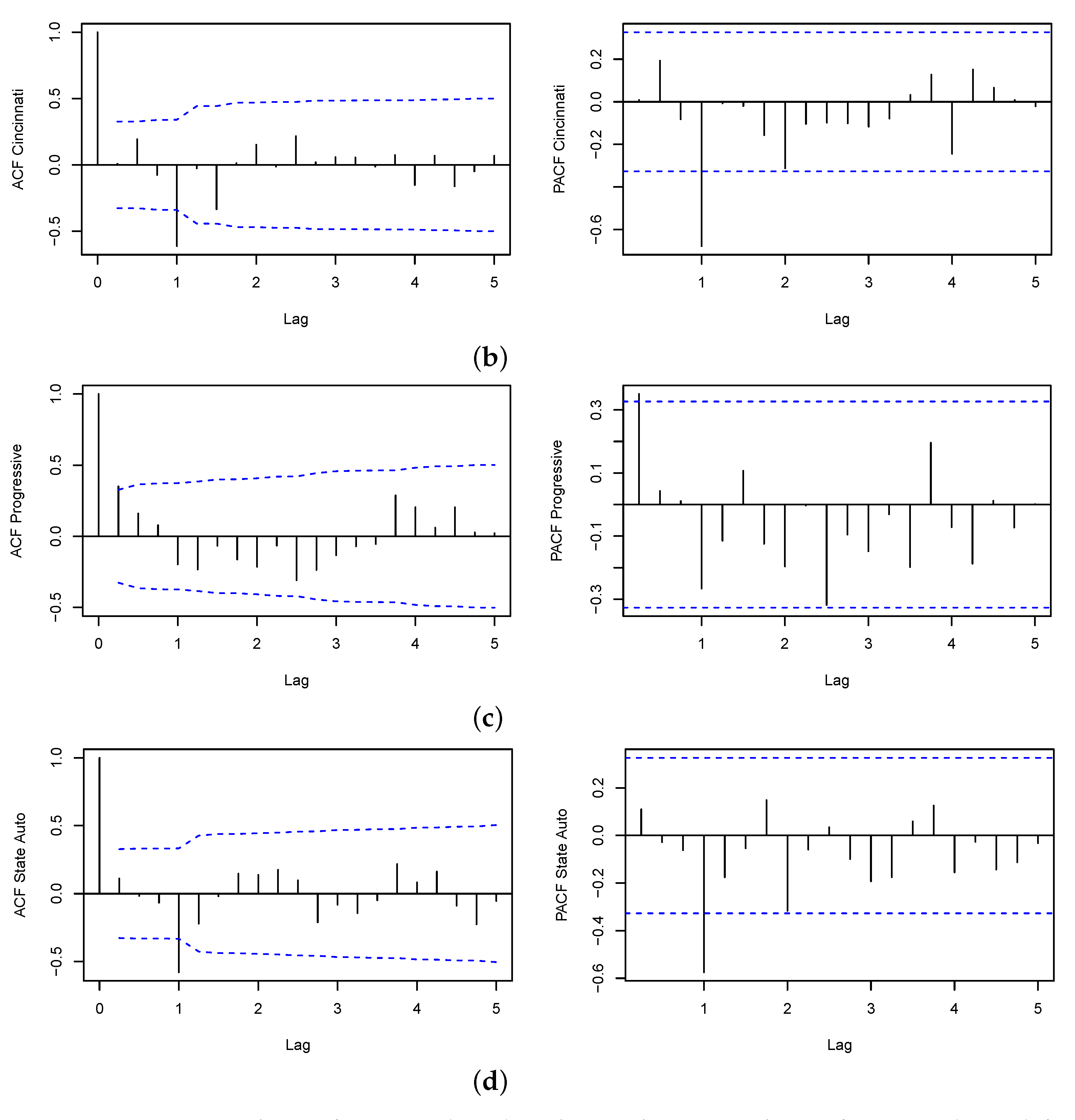
7.1. The Employed Models
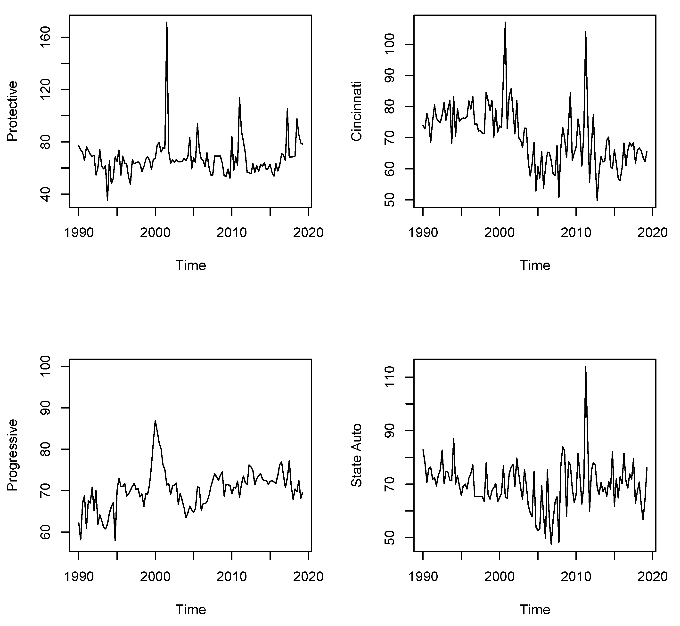
This section reports forecasting results with the proposed seasonal models and also considers autoregressive model specifications popular in the literature on underwriting cycles (Meier and Outreville 2006; Boyer et al. 2012). Previous research also considered polynomial trends. Instead, we use integrated ARMA models which can generate stochastic trend components due to the accumulation of shocks in time.19 Altogether, we explore
-
The AR[2] model,
-
The ARIMA[2,1,0] model,
-
At least two SARIMA specifications,
for each company under consideration.
Additionally, we evaluate forecasts from the corresponding intervention model variants. Throughout, we consider models with dummy variables marking the time that the catastrophes take place and instantaneous effects on loss ratio according to (3). These we denote using the suffix ‘D’, i.e., we evaluate for each company
-
The AR[2]-D model,
-
The ARIMA[2,1,0]-D model,
-
The corresponding SARIMA-D specifications, e.g., SARIMA[0,0,0]x[1,1,1]-D for Cincinnati.
In three cases, we also model the lingering depressing effect of certain catastrophes following model (5). These model variants are marked using the suffix ‘X’, e.g., SARIMA[0,0,0]x[1,1,1]-X for the Cincinnati data.20

7.2. The Forecasting Design

The forecasting procedure is as follows: We split our sample into 10 years in-sample data for 1990/Q1 through to 1999/Q4 used for model identification (a total of 40 observations) and 10 years out-of-sample data 2000/Q1—2019/Q2 used for forecast evaluation and backtesting. We first choose a number of appropriate model specifications based on the in-sample data. Second, we employ rolling window schemes for estimation of parameters and subsequent forecasting: We start by estimating a particular model up to time N, N ≥ 1999/Q4 and use the estimated parameter values to obtain forecasts for the loss ratio at time N + h with forecast horizons h = 1 , 2 , 4 , 8 quarters. In the next step, we roll the time window and estimate the model using data up to N + 1 and compute forecasts for the loss ratio at N + 1 + h. This is continued recursively until reaching the last observation in 2019/Q2. 21
In the case when a forecast deviates considerably from the true loss ratio, we register a “catastrophic event” in the data—this will coincide with a peak in the loss ratio plot. In this case, we model the major loss using an intervention variable. Suppose this happened at time N i . We then adjust our model by adding the intervention variable, e.g., we update the forecast model from SARIMA[0,0,0]x[1,1,1] to SARIMA[0,0,0]x[1,1,1]-D. We resume the recursive forecast scheme and calculate forecasts starting with N i + 1 . This adjustment procedure will be repeated each time a forecast fails.

7.3. Forecast Evaluation

We report empirical mean squared errors (MSE) and empirical mean absolute errors (MAE) for each forecast horizon h = 1 , 2 , 4 , 8 quarters (see Table 3 and Table 4).
Overall, our results indicate that models using intervention variables produce more accurate forecasts in terms of both MSE and MAE, as compared to the corresponding model version without intervention. Moreover, models with intervention variables provide best forecast results in the majority of cases under scrutiny. Figure 5 provides graphical representations of 1-step-ahead forecasts from our leading models. The main idea is that intervention models can separate between normal fluctuations and fluctuations attributable to a catastrophic event usually impossible to predict. This is most obvious in the case of Protective (top-left section) with high forecast errors during 2001–2002, when using the simple AR[2] model. By contrast, the AR[2]-X forecasts are much closer to the real data, the terrorist event of 9/11 being captured by a dummy variable and specifically handled in forecast calculations.
In general, intervention models produce more temperate forecasts and prevent severe forecast deviations due to major losses. In addition, seasonal models prove successful when data have a pronounced seasonal character, such as in the case of Cincinnati and State Auto (see Figure 5, top-right and bottom-right sections).
The case of Progressive constitutes an exception: the simple AR[2] model delivers best forecasting results for h 4 quarters, whereas any additional intervention variables prove non-profitable. This finding is reasonable if we consider that their loss ratio was less pronounced in the event year as compared to the other companies in the sample, the Progressive loss ratio having increased to less than 90% (see Figure 3). The small impact estimated in Section 6 also confirms this idea. Thus the AR[2] specification appears to be perfectly good in this case (see Figure 5, bottom-left section). According to our results, only in the long term, for 2-years-ahead forecasts, the AR[2]-D model provides lower MSE and MAE values.
We calculate model confidence sets for each forecast horizon based on the methodology in Hansen et al. (2011). Whereas empirical MSE and MAE values fluctuate subject to the realized data sample, model confidence sets have the advantage of providing forecast assessments with a certain confidence level. By analogy with a ( 1 α ) -confidence interval, the model confidence set (MCS) is a random subset of models containing the most accurate model with a probability no less than 1 α . By definition, the 100% MCS is the set containing all models under scrutiny, i.e., the set of all models contains the best model with 100% probability.
Table 5 contains the MCS p-values based on the evaluation of MSE values for each model under consideration and each forecast horizon. Similar results in terms of MAE are given in Table 6.22 A given model is contained in the ( 1 α ) confidence set if, and only if, its MCS p-value is no less than α . By construction, the model with an MCS p-value of 100% is contained in all confidence sets, i.e., it provides the most accurate forecasts. The results in Table 5 and Table 6 are computed from 1000 stationary bootstrap resamples of the original data following the procedure in Politis and Romano (1994).23
Overall, the MCS p-values reinforce the tendency expressed by our MSE and MAE results: intervention models prove most accurate forecasting capabilities in the great majority of cases. In the following, we discuss these results for each company. We cast an eye at the forecasting procedure based on intervention models in particular.
Protective
In the case of Protective the forecast model needed to be adjusted two times: First, we registered a considerable deviation between forecast and real loss ratio value at 2001/Q3. Therefore, we added a dummy variable with instantaneous effect β to the model. We resumed forecasting with this new model until next considerable forecast error at 2011/Q1. We estimated both an instantaneous and a lingering effect for this major loss. The new model takes both catastrophes into consideration. We resumed forecasts calculation for 2011/Q2 till sample end.
According to our MCS p-values in terms of MSE, only four models are contained in the 74% MCS at forecast horizons 1, 2, and 3 quarters, three of them being intervention models, which capture the effect of major losses explicitly. This indicates relatively pronounced differences in forecast precision against the remaining five models under scrutiny.
According to our results in Table 5, for each forecast horizon a different model provides the most accurate forecasts: The AR[2]-X model dominates the one-quarter-ahead forecasting exercise. For h = 2 and h = 3 two D-models come out best. In the long term, intervention variables prove to be immaterial, the simple AR[2] specification performing best.
In terms of the MCS p-values based on the MAE loss function (see Table 6), the AR[2]-X model provides the most accurate forecasts throughout and outperforms to a great extent its competitors.
Cincinnati
The intervention model for this company incorporates both catastrophes at 2000/Q4 and 2011/Q2. We estimate both an immediate and a lingering effect in each case. We report the best forecast results with the SARIMA-X model at horizons h 4 quarters, this being also the only specification in the 66% MCS in terms of MSE and definitely leading this competition. In the long term, the situation is less determinate, four different intervention models being contained in the 75% MCS based on MSE, with comparably high MCS p-values. The results in terms of MAE generate the same picture.
Progressive
We register only one major loss event at 2000/Q1 in the Progressive loss ratios. We estimate its effect using the intervention model (5) as in the case of Cincinnati. The simple AR[2] model delivers best forecasting results for h 4 quarters. For the one-quarter-ahead forecasts the AR[2] model is also the only specification contained in the 59% MCS in terms of MSE whereas the 67% MCS contains all models under scrutiny. Thus, the AR[2] dominates the competition, whereas the differences in forecast accuracy between the remaining eight models seem unpronounced. The situation is similar at horizons h = 2 and 4 quarters. Only in the case of two-years-ahead forecasts an intervention model, the AR[2]-D model, outperforms all competitors. The MCS p-values based on the MAE loss function provide similar findings.
State Auto
According to Figure 3, we do not distinguish any lingering effect after the major loss event at 2011/Q2 in the case of State Auto. Hence, we estimate model (3). According to the MCS p-values in terms of MSE the SARIMA[0,0,0]x[1,1,1]-D delivers throughout best results at all forecast horizons. These findings differ from those based on the evaluation of the MAE loss function only in the case h = 2 years, when the more simple AR[2] specification provides most accurate forecasts.

8. Conclusions

This article extends the literature on underwriting cycles in the property and casualty insurance industry. Following previous research, it challenges the question of existence and predictability of this phenomenon. Our results confirm the existence of underwriting cycles with a length of 8 to 9 years. Interestingly, this value is consistent with former findings (Grace and Hotchkiss 1995; Lazar and Denuit 2012; Meier and Outreville 2006; Owadally et al. 2019b). Since time series models require particularly large data samples to ensure reliable estimates, much longer time series are used than in previous studies containing quarterly company-based data. We also demonstrate that it is possible to increase forecasting performance by using an additional source of information: information on catastrophes or major losses.
Our analysis builds on the idea of (dis)connecting cycles and catastrophic events—which seems intuitive for modeling purposes since many catastrophes are unsystematic and rare events following autonomous dynamics. As a result, going beyond previous studies, we suggest that reliable forecasts should be performed net of the irregular peaks in loss distributions arising from natural and other catastrophes, as well as big ’unusual’ black swan events.
It is noteworthy that loss tails, i.e., the time frame that an insurance company needs to solve and settle its incoming claims, largely depend on the type of loss that occurred. As an example, in this paper we considered only two types of loss tail dynamics with immediate and lingering settlements. However, in practice, insurers have the possibility to estimate this loss tail more accurately depending on the type of major loss event. As a consequence, based on the intervention models introduced in this paper, insurers should be able to yield even superior forecasting performance when modeling and predicting underwriting cycles.

Author Contributions

Methodology, A.H. and C.S.; Investigation, A.H. and C.S.; Writing—original draft, A.H. and C.S.; Writing—review and editing, A.H. and C.S. All authors have read and agreed to the published version of the manuscript.

Funding

C.S. is grateful for having been invited to St. John’s University, Maurice R. Greenberg School of Risk Management, Insurance, and Actuarial Science as Berkley Scholar.

Data Availability Statement

The data presented in this study are available upon request to the corresponding author.

Conflicts of Interest

The authors declare no conflict of interest.

Appendix A. Regression Diagnostics

These are regression diagnostics for model (1). The following table contains our regression output including the estimated values for a and b in column “Parameter Est”. Note that both parameters are significant at acceptable levels of significance. Figure A1 displays the fitted harmonic model where a determines the height (or amplitude) of the cycle and b its phase, i.e., the location of the first peak. The model residuals have only two significant autocorrelations (see Figure A2, right section). Overall, the model seems to fit well to the data.
Moreover, we cannot reject the null hypothesis of normal residuals using the Shapiro–Wilk normality test (p-value = 0.766). This result is also confirmed by the QQ-diagram in Figure A2 (left section).
Table A1. Regression output for model (1).
Variable Parameter Est. Std. Errort-Testp-Value
cos 2 π λ t 3.795 0.6675.6906.6 × 10 7 **
sin 2 π λ t 1.323 0.6671.9840.0528 *
Multiple R 2 : 0.421Adjusted R 2 : 0.398
p-value F-test: 1.18 × 10 6
(Note: significance level: ** = 0.01, * = 0.10).
Figure A1. Fitted model.
Risks 11 00075 g0a1
Figure A2. Residual diagnostics.
Risks 11 00075 g0a2

Appendix B. ACF and PACF Plots

Figure A3. Autocorrelation functions (ACF) and partial autocorrelation functions (PACF) for the seasonally differenced loss ratios for four insurance companies: (a) Protective, (b) Cincinnati, (c) Progressive and (d) State Auto. Note: All series have been logarithmically transformed first.
Risks 11 00075 g0a3aRisks 11 00075 g0a3b

Notes

1
See, for instance, Adam and Merkel (2019), as well as Harrington and Niehaus (2000).
2
See, for instance, Marx (2013), as well as Harrington and Niehaus (2000).
3
Note that the benchmark autoregressive model can also generate cycles.
4
Note that unit roots are not compatible with the loss ratio dynamics of insurance companies per se.
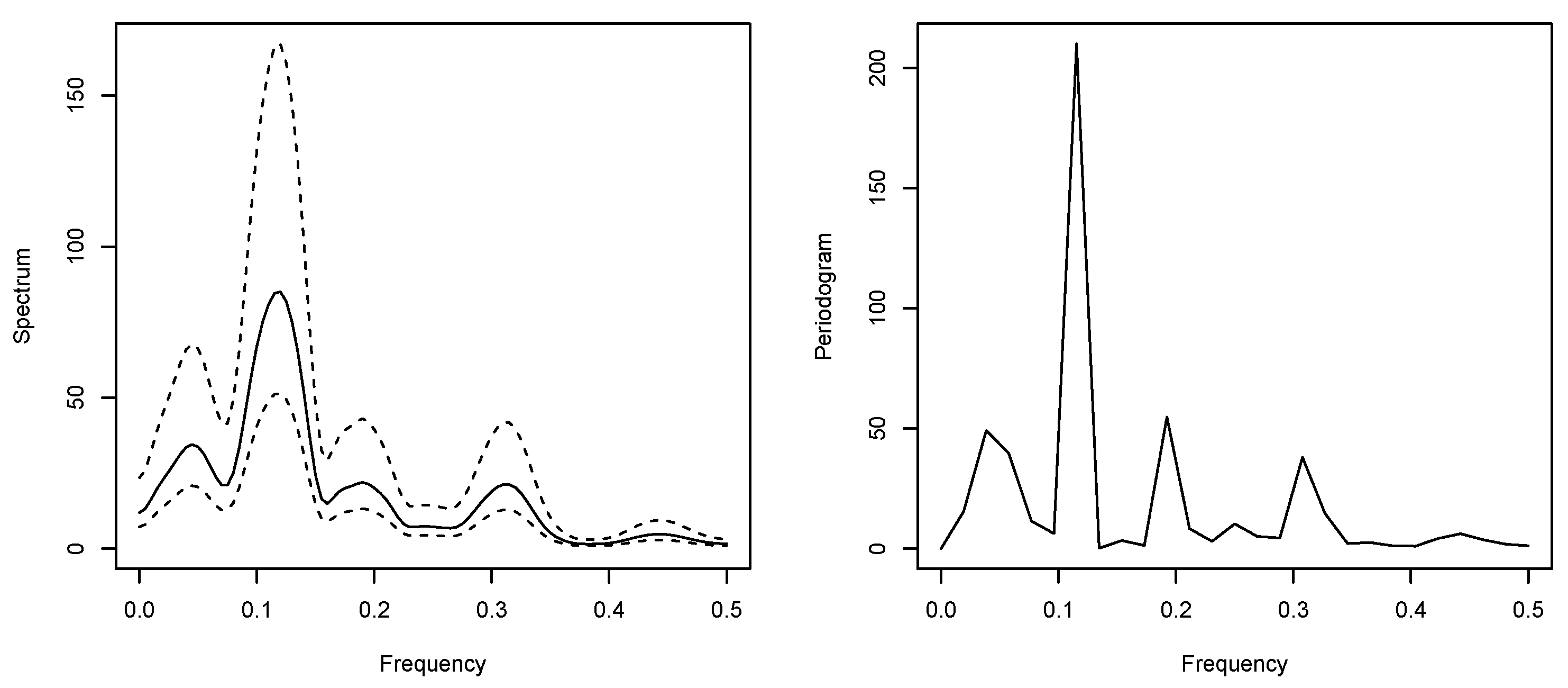
5
Cycle analysis results based on the estimation of autoregressive models have proven of poor statistical significance due to the particularly short time series available in the insurance industry (Boyer and Owadally 2015; Boyer et al. 2012; Owadally et al. 2019b; Venezian and Leng 2006). On account of this we abstain from any evaluation of cycles based on these models in this paper. Instead, we set the focus on short- and mid-term forecasts and on the evaluation of intervention effects using quarterly underwriting data.
6
An early paper by Venezian (1985) argues that institutional rigidities may be the cause of the underwriting cycle in the sense that systematic errors in projecting premiums on the basis of prior loss experience generates fluctuations in future profitability in the insurance industry.
7
Note that in a perfect insurance market, insurers can adjust their capital to bring down insolvency risk.
8
Mourdoukoutas et al. (2022) propose a multi-stage insurance game with observable actions, implying open-loop and closed-loop equilibrium premium profiles that might be cyclical in nature. However, cycles may not always occur, as demonstrated by Wang and Murdock (2019). The impact of a loss shock on an insurer’s cash flows might spread out and amplify over time due to the interaction between its underwriting capability and ability to raise external capital, generating a non-cyclical pattern of changes in underwriting coverage and access to external capital.
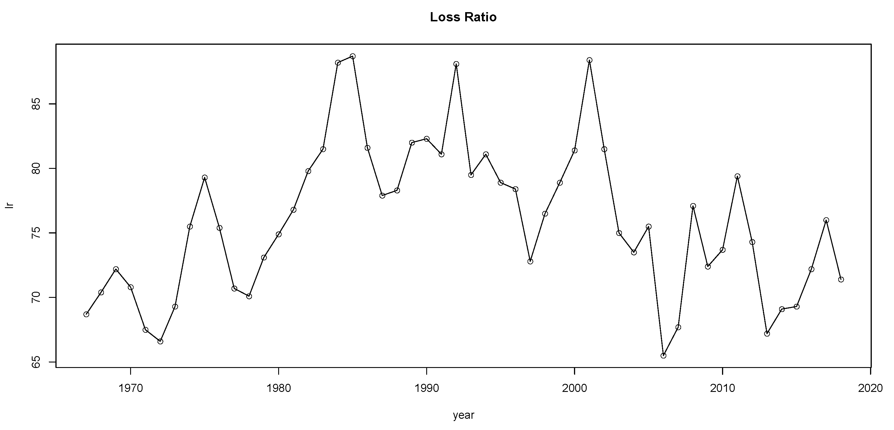
9
The annual loss ratio is defined as insurance claims paid plus adjustment expenses divided by total earned premiums for a given year.
10
See also Brockwell and Davis (1991) for a brief overview.
11
As a matter of fact, the authors report higher power for their test procedure compared to Fisher’s test even in the case of Gaussian data. The robust test of Ahdesmäki et al. (2005) was implemented with package ‘ptest’ by Lai and McLeod (2016) using R (R Core Team 2020). Lai and McLeod (2016) calculate p-values with the response surface regression method (MacKinnon 2002) which is more accurate and computationally more efficient than the time-consuming simulation method.
12
The term autoregressive in ARIMA refers to a linear regression model that uses its own lags as predictors.
13
Note that the intervention model can be easily extended to capture any loss reporting delay.
14
Given the particular regulatory framework of the insurance industry, permanent effects on loss ratios are not reasonable, e.g., one cannot assume that catastrophes would induce a permanent shift in the mean level. Following these considerations we only use pulse dummy variables to model catastrophes.
15
The plots of the relevant autocorrelation functions (ACF) and partial autocorrelation functions (PACF) can be found in Appendix B.
16
Bloomberg provides quarterly data on 63 companies in the property and casualty business traded and domiciled in the US. We selected only those companies with fairly large series, starting in the first quarter 1990 at the latest, i.e., with at least 118 observations. We checked our data against annual company data from SNL and selected only the series consistent for both data sources in order to avoid potentially false information.
17
Throughout, models were fitted to the series of logarithmic loss ratio values to stabilize variance. We employed package TSA by Chan and Ripley (2020) using R (R Core Team 2020).
18
The parameter β ( 2 ) for the dummy variable flagging the time point 2011/Q1 of the second event is not statistically significant, and so we removed it from the model.
19
Note that the estimation of a polynomial trend might have severe consequences on inference results, e.g., the significance level (probability of error) α might no longer be satisfied. See Chan et al. (1977), Nelson and Kang (1981), as well as Nelson and Kang (1984).
20
We employed the R package TSA by Chan and Ripley (2020) using R (R Core Team 2020).
21
We fit our models to the logarithmic loss ratios and convert forecasts back into forecasts of absolute loss ratio for the purpose of evaluation.
22
We employed the MFE Toolbox by Sheppard (2009) using MATLAB (MathWorks 2018).
23
We have also experimented with a higher number of bootstrap replications, as well as with the circular block bootstrap leading to irrelevant results changes.

References

  1. Adam, Klaus, and Sebastian Merkel. 2019. Stock Price Cycles and Business Cycles. Available online: https://ssrn.com/abstract=3329820 (accessed on 10 December 2022).
  2. Ahdesmäki, Miika, Harri Lähdesmäki, Ron Pearson, Heikki Huttunen, and Olli Yli-Harja. 2005. Robust detection of periodic time series measured from biological systems. BMC Bioinformatics 6: 1–18. [Google Scholar] [CrossRef] [PubMed] [Green Version]
  3. Artis, Michael J., Mathias Hoffmann, Dilip M. Nachane, and Juan Toro. 2004. The Detection of Hidden Periodicities: A Comparison of Alternative Methods. Working Paper EUI ECO, 2004/10. Fiesole: European University Institute. [Google Scholar]
  4. Bartlett, Maurice S. 1957. Discussion on symposium on spectral approach to time series. Journal of the Royal Statistical Society: Series B 19: 1–63. [Google Scholar]
  5. Bølviken, Erik. 1983. New tests of significance in periodogram analysis. Scandinavian Journal of Statistics 1: 1–9. [Google Scholar]
  6. Boonen, Tim J., Athanasios A. Pantelous, and Renchao Wu. 2018. Non-cooperative dynamic games for general insurance markets. Insurance: Mathematics and Economics 78: 123–35. [Google Scholar] [CrossRef] [Green Version]
  7. Box, George E. P., and George C. Tiao. 1975. Intervention analysis with applications to economic and environmental problems. Journal of the American Statistical Association 70: 70–79. [Google Scholar] [CrossRef]
  8. Box, George E. P., and Gwilym M. Jenkins. 1970. Time Series Analysis, Forecasting and Control. San Francisco: Holden-Day. [Google Scholar]
  9. Boyer, M. Martin, and Iqbal Owadally. 2015. Underwriting apophenia and cryptids: Are cycles statistical figments of our imagination? Geneva Papers on Risk and Insurance—Issues and Practice 40: 232–55. [Google Scholar] [CrossRef] [Green Version]
  10. Boyer, M. Martin, Eric Jacquier, and Simon Van Norden. 2012. Are underwriting cycles real and forecastable? Journal of Risk and Insurance 79: 995–1015. [Google Scholar] [CrossRef]
  11. Brockwell, Peter J., and Richard. A. Davis. 1991. Time Series: Theory and Methods, 2nd ed. New York: Springer. [Google Scholar]
  12. Browne, Mark J., Lan Ju, and Zhiyong Tu. 2014. Broker monitoring of premium adequacy: The role of contingent commissions. Applied Economics 46: 2375–86. [Google Scholar] [CrossRef]
  13. Cagle, Julie A. B., and Scott E. Harrington. 1996. Insurance supply with capacity constraints and endogenous insolvency risk. Insurance Mathematics and Economics 2: 148. [Google Scholar] [CrossRef]
  14. Canova, Fabio. 1996. Three tests for the existence of cycles in time series. Ricerche Economiche 50: 135–62. [Google Scholar] [CrossRef]
  15. Chan, K. Hung, Jack C. Hayya, and J. Keith Ord. 1977. A note on trend removal methods—The case of polynomial versus variate differencing. Econometrica 45: 737–44. [Google Scholar] [CrossRef]
  16. Chan, Kung-Sik, and Brian Ripley. 2020. TSA: Time Series Analysis. R Package Version 1.3. Available online: https://cran.r-project.org/web/packages/TSA/index.html (accessed on 9 October 2020).
  17. Chatfield, Chris. 1993. Calculating interval forecasts. Journal of Business & Economic Statistics 11: 121–35. [Google Scholar]
  18. Chiu, Shean-Tsong. 1989. Detecting periodic components in a white gaussian time series. Journal of the Royal Statistical Society: Series B (Methodological) 51: 249–59. [Google Scholar] [CrossRef]
  19. Cryer, Jonathan D., and Kung-Sik Chan. 2010. Time Series Analysis. With Applications in R, 2nd ed.New York: Springer. [Google Scholar]
  20. Cummins, J. David, and David W. Sommer. 1996. Capital and risk in property-liability insurance markets. Journal of Banking & Finance 20: 1069–92. [Google Scholar]
  21. Cummins, J. David, and J. Francois Outreville. 1987. An international analysis of underwriting cycles in property-liability insurance. Journal of Risk and Insurance 54: 246–62. [Google Scholar] [CrossRef]
  22. Doherty, Neil A., and Han Bin Kang. 1988. Interest rates and insurance price cycles. Journal of Banking & Finance 12: 199–214. [Google Scholar]
  23. Doherty, Neil A., and James R. Garven. 1995. Insurance cycles: Interest rates and the capacity constraint model. Journal of Business 68: 383–404. [Google Scholar] [CrossRef]
  24. Doherty, Neil A., and Lisa Posey. 1997. Availability crises in insurance markets: Optimal contracts with asymmetric information and capacity constraints. Journal of Risk and Uncertainty 15: 55–80. [Google Scholar] [CrossRef]
  25. Fisher, Ronald A. 1929. Tests of significance in harmonic analysis. Proceedings of the Royal Society of London. Series A 125: 54–59. [Google Scholar]
  26. Fung, Hung-Gay, Gene C. Lai, Gary A. Patterson, and Robert C. Witt. 1998. Underwriting cycles in property and liability insurance: An empirical analysis of industry and by-line data. Journal of Risk and Insurance 65: 539–61. [Google Scholar] [CrossRef]
  27. Grace, Martin F., and Julie L. Hotchkiss. 1995. External impacts on the property-liability insurance cycle. Journal of Risk and Insurance 62: 738–54. [Google Scholar] [CrossRef] [Green Version]
  28. Gron, Anne. 1994a. Capacity constraints and cycles in property-casualty insurance markets. The RAND Journal of Economics 25: 110–27. [Google Scholar] [CrossRef]
  29. Gron, Anne. 1994b. Evidence of capacity constraints in insurance markets. The Journal of Law and Economics 37: 349–77. [Google Scholar] [CrossRef]
  30. Guo, Feng, Hung-Gay Fung, and Ying Sophie Huang. 2009. The dynamic impact of macro shocks on insurance premiums. Journal of Financial Services Research 35: 225–44. [Google Scholar] [CrossRef]
  31. Hannan, Eduard J. 1961. Testing for a jump in the spectral function. Journal of the Royal Statistical Society: Series B (Methodological) 23: 394–404. [Google Scholar]
  32. Hansen, Peter, Asger Lunde, and James Nason. 2011. The model confidence set. Econometrica 79: 453–97. [Google Scholar] [CrossRef] [Green Version]
  33. Harrington, Scott E., and Greg Niehaus. 2000. Volatility and underwriting cycles. In Handbook of Insurance. Berlin: Springer, pp. 657–86. [Google Scholar] [CrossRef]
  34. Harrington, Scott E., and Patricia M. Danzon. 1994. Price cutting in liability insurance markets. Journal of Business 67: 511–38. [Google Scholar]
  35. Harrington, Scott E., Greg Niehaus, and Tong Yu. 2013. Insurance price volatility and underwriting cycles. In Handbook of Insurance. Berlin: Springer, pp. 647–67. [Google Scholar] [CrossRef]
  36. Hohensinn, Roland, Simon Häberling, and Alain Geiger. 2020. Dynamic displacements from high-rate gnss: Error modeling and vibration detection. Measurement 157: 107655. [Google Scholar] [CrossRef]
  37. Jawadi, Fredj, Catherine Bruneau, and Nadia Sghaier. 2009. Nonlinear cointegration relationships between non-life insurance premiums and financial markets. Journal of Risk and Insurance 76: 753–83. [Google Scholar] [CrossRef]
  38. Jiang, Shi-jie, and Chien-Chung Nieh. 2012. Dynamics of underwriting profits: Evidence from the u.s. insurance market. International Review of Economics & Finance 21: 1–15. [Google Scholar]
  39. Kay, Steven M., and Stanley Lawrence Marple. 1981. Spectrum analysis—A modern perspective. Proceedings of the IEEE 69: 1380–419. [Google Scholar] [CrossRef]
  40. Lai, Yuanhao, and A. Ian McLeod. 2016. ptest: Periodicity Tests in Short Time Series. R Package Version 1.0-8. Available online: https://cran.r-project.org/web/packages/ptest/index.html (accessed on 12 August 2021).
  41. Lamm-Tennant, Joan, and Mary A. Weiss. 1997. International insurance cycles: Rational expectations/institutional intervention. Journal of Risk and Insurance 64: 415–39. [Google Scholar] [CrossRef]
  42. Lazar, Dorina, and Michel M. Denuit. 2012. Multivariate analysis of premium dynamics in p&l insurance. Journal of Risk and Insurance 79: 431–48. [Google Scholar]
  43. Lei, Yu, and Mark J. Browne. 2017. Underwriting strategy and the underwriting cycle in medical malpractice insurance. The Geneva Papers on Risk and Insurance-Issues and Practice 42: 152–75. [Google Scholar] [CrossRef]
  44. MacKinnon, James G. 2002. Computing numerical distribution functions in econometrics. In High Performance Computing Systems and Applications. Berlin: Springer, pp. 455–71. [Google Scholar]
  45. Malinovskii, Vsevolod K. 2010. Competition-originated cycles and insurance strategies. ASTIN Bulletin: The Journal of the IAA 40: 797–843. [Google Scholar]
  46. Marx, Brian. 2013. Hard Market vs. Soft Market: The Insurance Industry’s Cycle and Why We Are Currently in a Hard Market. PSA Financial. Available online: https://www.psafinancial.com/2013/01/hard-market-vs-soft-market-the-insurance-industrys-cycle-and-why-were-currently-in-a-hard-market/ (accessed on 15 December 2022).
  47. MathWorks. 2018. MATLAB R2018a. Available online: http://www.mathworks.com/ (accessed on 9 April 2020).
  48. McSweeney, Laura A. 2006. Comparison of periodogram tests. Journal of Statistical Computation and Simulation 76: 357–69. [Google Scholar] [CrossRef]
  49. Meier, Ursina B. 2006. Multi-national underwriting cycles in property-liability insurance: Part I—Some theory and empirical results. The Journal of Risk Finance 7: 64–82. [Google Scholar] [CrossRef]
  50. Meier, Ursina B., and J. François Outreville. 2006. Business cycles in insurance and reinsurance: The case of france, germany and switzerland. The Journal of Risk Finance 7: 160–76. [Google Scholar] [CrossRef]
  51. Mourdoukoutas, Fotios, Athanasios A. Pantelous, and Greg Taylor. 2022. Competitive Insurance Pricing Strategies for Multiple Lines of Business: A Game Theoretic Approach. Available online: https://papers.ssrn.com/sol3/papers.cfm?abstract_id=4049437 (accessed on 10 December 2022).
  52. Nelson, Charles R., and Heejoon Kang. 1981. Spurious periodicity in inappropiately detrended time series. Econometrica 49: 741–51. [Google Scholar] [CrossRef] [Green Version]
  53. Nelson, Charles R., and Heejoon Kang. 1984. Pitfalls in the use of time as an explanatory variable in regression. Journal of Business & Economic Statistics 2: 73–82. [Google Scholar]
  54. Niehaus, Greg, and Andy Terry. 1993. Evidence on the time series properties of insurance premiums and causes of the underwriting cycle: New support for the capital market imperfection hypothesis. Journal of Risk and Insurance 60: 466–79. [Google Scholar] [CrossRef]
  55. Owadally, Iqbal, Feng Zhou, and Douglas Wright. 2018. The insurance industry as a complex social system: Competition, cycles, and crises. Journal of Artificial Societies and Social Simulation 21: 2. [Google Scholar] [CrossRef]
  56. Owadally, Iqbal, Feng Zhou, Rasaq Otunba, Jessica Lin, and Douglas Wright. 2019a. An agent-based system with temporal data mining for monitoring financial stability on insurance markets. Expert Systems with Applications 123: 270–82. [Google Scholar] [CrossRef]
  57. Owadally, Iqbal, Feng Zhou, Rasaq Otunba, Jessica Lin, and Douglas Wright. 2019b. Time series data mining with an application to the measurement of underwriting cycles. North American Actuarial Journal 23: 469–84. [Google Scholar] [CrossRef]
  58. Pisarenko, Vladilen F. 1973. The retrieval of harmonics from a covariance function. Geophysical Journal International 33: 347–66. [Google Scholar] [CrossRef] [Green Version]
  59. Politis, Dimitris N., and Joseph P. Romano. 1994. The stationary bootstrap. Journal of the American Statistical Association 89: 1303–13. [Google Scholar] [CrossRef]
  60. R Core Team. 2020. R: A Language and Environment for Statistical Computing. Vienna: R Foundation for Statistical Computing. Available online: http://www.R-project.org/ (accessed on 9 April 2020).
  61. Sheppard, Kevin. 2009. MFE Toolbox, Version 4.0. Available online: https://www.kevinsheppard.com/code/matlab/mfe-toolbox/ (accessed on 9 April 2020).
  62. Siegel, Andrew F. 1980. Testing for periodicity in a time series. Journal of the American Statistical Association 75: 345–48. [Google Scholar] [CrossRef]
  63. Telesca, Luciano, Alessandro Giocoli, Vincenzo Lapenna, and Tony Alfredo Stabile. 2015. Robust identification of periodic behavior in the time dynamics of short seismic series: The case of seismicity induced by pertusillo lake, southern italy. Stochastic Environmental Research and Risk Assessment 29: 1437–46. [Google Scholar] [CrossRef]
  64. Venezian, Emilio C. 1985. Ratemaking methods and profit cycles in property and liability insurance. Journal of Risk and Insurance 52: 477–500. [Google Scholar] [CrossRef]
  65. Venezian, Emilio C. 2006. The use of spectral analysis in insurance cycle research. The Journal of Risk Finance 7: 177–88. [Google Scholar] [CrossRef]
  66. Venezian, Emilio C., and Chao-Chun Leng. 2006. Application of spectral and arima analysis to combined-ratio patterns. The Journal of Risk Finance 7: 189–214. [Google Scholar] [CrossRef]
  67. Wang, Ning, and Maryna Murdock. 2019. A dynamic model of an insurer: Loss shocks, capacity constraints and underwriting cycles. The Journal of Risk Finance 20: 82–93. [Google Scholar] [CrossRef]
  68. Wang, Shaun S., John A. Major, Charles H. Pan, and Jessica W. K. Leong. 2011. Us property-casualty: Underwriting cycle modeling and risk benchmarks. Variance 5: 91–114. [Google Scholar]
  69. Whittle, Peter. 1952. Tests of fit in time series. Biometrika 39: 309–18. [Google Scholar] [CrossRef]
  70. Winter, Ralph A. 1988. The liability crisis and the dynamics of competitive insurance markets. Yale Journal on Regulation 5: 455. [Google Scholar]
  71. Winter, Ralph A. 1994. The dynamics of competitive insurance markets. Journal of Financial Intermediation 3: 379–415. [Google Scholar] [CrossRef]
  72. Yilmaz, A. K. D. İ., Serdar Varlik, and Hakan Berument. 2018. Cycle duration in production with periodicity—Evidence from Turkey. International Econometric Review 10: 24–32. [Google Scholar]
Figure 1. Loss ratios in the property and casualty insurance industry in the U.S. over 52 years, 1967–2018. (Source: Best’s Aggregates and Averages).
Risks 11 00075 g001
Figure 2. Direct smoothed spectral estimation with Bartlett–Priestley window and approximate confidence intervals (left), and scaled periodogram (right) for the detrended annual loss ratios.
Risks 11 00075 g002
Figure 3. Quarterly loss ratio data for four insurance companies: 1990/Q1–2019/Q2. (Source: Bloomberg).
Risks 11 00075 g003
Figure 4. Fitted model (left) and estimated effects of catastrophes on the logarithmic loss ratios (right) for the companies (a) Protective, (b) Cincinnati, and (c) Progressive.
Risks 11 00075 g004
Figure 5. One-quarter ahead loss ratio forecasts for four insurance companies: 2000/Q1–2019/Q2. (Note: Throughout, real data displayed in black. According to our results, forecasts from intervention models outperform AR[2] forecasts for the companies Protective, Cincinnati, and State Auto. This situation changes in the case of Progressive with superior AR[2] forecasts).
Risks 11 00075 g005
Table 1. Data description.
Quarterly Loss Ratios on US Property and Casualty Companies
CompanyNo. Obs.No Obs.Cat 1Cat 2
Pre-Interv.
Protective118462001/Q32011/Q1
Cincinnati118432000/Q42011/Q2
Progressive118402000/Q1
State Auto118852011/Q2
(Note: Quarterly data for four insurance companies, sample: 1990/Q1–2019/Q2, source: Bloomberg).
Table 2. Estimation results: coefficients and standard errors in parentheses.
SARIMA Parameters
Intercept ϕ 1 ϕ 2 ψ 1
PROT.  4.1802 ** 0.2394 ** 0.2793 **
(0.0248)(0.0889)(0.0902)
CINC.   0.4062 **
(0.1050)
PROGR. 4.2407 ** 0.5601 ** 0.2272 *
(0.0178)(0.0911)(0.0934)
Intervention Parameters
β ( 1 ) ω ( 1 ) δ ( 1 ) ω ( 2 ) δ ( 2 )
PROT.  0.8996 ** 0.5631 ** 0.5546 **
(0.1223) (0.1239)(0.1325)
CINC.   0.2460 * 0.1593 * 0.8152 **
(0.1005)(0.0725)(0.0751)
PROGR. 0.1127 ** 0.7806 **
(0.0423)(0.1559)
(Note: significance level: ** = 0.01, * = 0.05).
Table 3. Root mean squared errors of forecasts of underwriting ratios for the companies, Protective, Cincinnati, Progressive, and State Auto, forecast horizons h = 1 , 2 , 4 and 8 quarters. Best forecasts in bold type.
Root Mean Squared Errors of Forecasts of Underwriting Ratios
Modelh = 1 Quarterh = 2 Quartersh = 4 Quartersh = 8 Quarters
PROTECTIVE
AR[2]16.4417.0317.1512.02
AR[2]-D15.9816.4416.9412.09
ARIMA[2,1,0]17.6518.4119.0016.90
ARIMA[2,1,0]-D16.0716.7016.6914.35
SARIMA[0,0,0]x[2,1,0]18.6518.8618.9515.40
SARIMA[0,0,0]x[2,1,0]-D17.4317.5817.6113.92
SARIMA[0,0,0]x[0,1,1]18.1918.4118.4613.71
SARIMA[0,0,0]x[0,1,1]-D17.4517.5617.5412.57
AR[2]-X15.9416.4516.9712.14
CINCINNATI
AR[2]9.6710.4410.2210.90
AR[2]-D9.509.909.6910.36
ARIMA[2,1,0]9.279.979.8810.58
ARIMA[2,1,0]-D9.029.459.089.17
SARIMA[0,0,0]x[0,1,1]9.159.339.5910.41
SARIMA[0,0,0]x[0,1,1]-D8.578.668.939.39
SARIMA[0,0,0]x[1,1,1]9.319.8210.1111.00
SARIMA[0,0,0]x[1,1,1]-D8.768.859.189.30
SARIMA[0,0,0]x[0,1,1]-X8.508.558.829.30
PROGRESSIVE
AR[2]2.512.842.973.45
AR[2]-D2.702.983.023.39
ARIMA[2,1,0]2.583.103.714.92
ARIMA[2,1,0]-D2.643.043.534.63
SARIMA[1,0,0]x[0,1,0]3.043.613.865.22
SARIMA[1,0,0]x[0,1,0]-D3.193.473.584.70
SARIMA[0,0,1]x[0,1,0]3.373.973.685.02
SARIMA[0,0,1]x[0,1,0]-D3.513.783.504.57
AR[2]-X2.753.063.103.52
STATE AUTO
AR[2]10.2010.3310.1010.75
AR[2]-D10.3710.2810.1210.76
ARIMA[2,1,0]10.5310.6210.2611.90
ARIMA[2,1,0]-D10.6710.2310.1511.51
SARIMA[0,0,0]x[1,1,0]10.0310.0910.1512.38
SARIMA[0,0,0]x[1,1,0]-D9.389.429.4811.56
SARIMA[0,0,0]x[0,1,1]9.709.739.8411.65
SARIMA[0,0,0]x[0,1,1]-D9.269.279.3711.05
SARIMA[0,0,0]x[1,1,1]9.229.289.4210.95
SARIMA[0,0,0]x[1,1,1]-D9.009.059.1710.70
(Note: Intervention models with an instantaneous effect on loss ratio at the time point of the catastrophic outbreak were marked using the suffix ‘D’. Intervention models with a lingering depressing effect, when loss ratios would recover gradually after a catastrophe, were marked using the suffix ‘X’. Throughout, the involved dummy variables flag the time point when the catastrophe takes place).
Table 4. Mean absolute errors of forecasts of underwriting ratios for the companies, Protective, Cincinnati, Progressive, and State Auto, forecast horizons h = 1 , 2 , 4 and 8 quarters. Best forecasts in bold type.
Mean Absolute Errors of Forecasts of Underwriting Ratios
Modelh = 1 Quarterh = 2 Quartersh = 4 Quartersh = 8 Quarters
PROTECTIVE
AR[2]8.659.219.668.10
AR[2]-D8.188.699.187.94
ARIMA[2,1,0]10.1510.9412.0411.95
ARIMA[2,1,0]-D8.939.7710.2910.19
SARIMA[0,0,0]x[2,1,0]11.6411.8711.7310.78
SARIMA[0,0,0]x[2,1,0]-D10.3210.4810.339.81
SARIMA[0,0,0]x[0,1,1]10.4510.7310.459.04
SARIMA[0,0,0]x[0,1,1]-D9.839.939.708.34
AR[2]-X8.048.689.157.92
CINCINNATI
AR[2]6.917.797.898.98
AR[2]-D6.857.387.418.25
ARIMA[2,1,0]6.637.277.128.02
ARIMA[2,1,0]-D6.677.016.617.12
SARIMA[0,0,0]x[0,1,1]6.837.057.268.05
SARIMA[0,0,0]x[0,1,1]-D6.416.536.757.35
SARIMA[0,0,0]x[1,1,1]7.167.567.828.56
SARIMA[0,0,0]x[1,1,1]-D6.656.777.067.34
SARIMA[0,0,0]x[0,1,1]-X6.286.386.577.23
PROGRESSIVE
AR[2]1.842.182.392.91
AR[2]-D1.942.282.412.85
ARIMA[2,1,0]1.912.452.753.83
ARIMA[2,1,0]-D1.952.412.653.73
SARIMA[1,0,0]x[0,1,0]2.242.692.853.94
SARIMA[1,0,0]x[0,1,0]-D2.292.672.703.74
SARIMA[0,0,1]x[0,1,0]2.442.912.743.85
SARIMA[0,0,1]x[0,1,0]-D2.432.782.653.64
AR[2]-X2.032.362.532.94
STATE AUTO
AR[2]7.647.627.507.89
AR[2]-D7.787.587.517.91
ARIMA[2,1,0]8.088.147.789.34
ARIMA[2,1,0]-D8.097.747.568.92
SARIMA[0,0,0]x[1,1,0]7.747.847.849.78
SARIMA[0,0,0]x1,1,0]-D7.317.397.369.30
SARIMA[0,0,0]x[0,1,1]7.497.587.659.14
SARIMA[0,0,0]x[0,1,1]-D7.087.137.198.69
SARIMA[0,0,0]x[1,1,1]6.826.927.048.31
SARIMA[0,0,0]x[1,1,1]-D6.646.726.808.04
(Note: Intervention models with an instantaneous effect on loss ratio at the time point of the catastrophic outbreak were marked using the suffix ‘D’. Intervention models with a lingering depressing effect, when loss ratios would recover gradually after a catastrophe, were marked using the suffix ‘X’. Throughout, the involved dummy variables flag the time point when the catastrophe takes place).
Table 5. MCS p-values with respect to the MSE values of forecasts of underwriting ratios based on 1000 stationary bootstrap resamples for the companies, Protective, Cincinnati, Progressive, and State Auto, and for each of the forecasting horizons h = 1 , 2 , 4 and 8 quarters. Forecasts in the 90% MCS in bold type.
MCS p-Values Based on the MSE as a Loss Function
Modelh = 1 Quarterh = 2 Quartersh = 4 Quartersh = 8 Quarters
PROTECTIVE
AR[2]0.780.790.601.00
AR[2]-D0.781.000.800.58
ARIMA[2,1,0]0.200.010.0150.00
ARIMA[2,1,0]-D0.780.831.000.04
SARIMA[0,0,0]x[2,1,0]0.200.260.0150.05
SARIMA[0,0,0]x[2,1,0]-D0.200.260.200.05
SARIMA[0,0,0]x[0,1,1]0.010.010.020.00
SARIMA[0,0,0]x[0,1,1]-D0.020.010.020.00
AR[2]-X1.000.830.600.58
CINCINNATI
AR[2]0.060.030.000.00
AR[2]-D0.070.030.080.25
ARIMA[2,1,0]0.110.090.080.25
ARIMA[2,1,0]-D0.110.090.341.00
SARIMA[0,0,0]x[0,1,1]0.110.090.080.16
SARIMA[0,0,0]x[0,1,1]-D0.300.120.340.83
SARIMA[0,0,0]x[1,1,1]0.070.030.000.00
SARIMA[0,0,0]x[1,1,1]-D0.110.090.081.00
SARIMA[0,0,0]x[0,1,1]-X1.00.1.001.000.96
PROGRESSIVE
AR[2]1.001.001.000.70
AR[2]-D0.400.520.411.00
ARIMA[2,1,0]0.400.520.410.54
ARIMA[2,1,0]-D0.400.520.410.54
SARIMA[0,0,1]x[0,1,0]0.330.270.410.54
SARIMA[0,0,1]x[0,1,0]-D0.330.230.410.54
SARIMA[1,0,0]x[0,1,0]0.330.520.110.37
SARIMA[1,0,0]x[0,1,0]-D0.330.520.110.29
AR[2]-X0.330.520.410.70
STATE AUTO
AR[2]0.160.200.340.92
AR[2]-D0.160.220.340.78
ARIMA[2,1,0]0.090.200.270.01
ARIMA[2,1,0]-D0.160.200.340.16
SARIMA[0,0,0]x[0,1,1]0.160.220.340.33
SARIMA[0,0,0]x[0,1,1]-D0.190.270.450.55
SARIMA[0,0,0]x[1,1,0]0.160.200.270.06
SARIMA[0,0,0]x[1,1,0]-D0.190.220.450.10
SARIMA[0,0,0]x[1,1,1]0.520.270.450.66
SARIMA[0,0,0]x[1,1,1]-D1.001.001.001.00
(Note: Intervention models with an instantaneous effect on loss ratio at the time point of the catastrophic outbreak were marked using the suffix ‘D’. Intervention models with a lingering depressing effect, when loss ratios would recover gradually after a catastrophe, were marked using the suffix ‘X’. Throughout, the involved dummy variables flag the time point when the catastrophe takes place).
Table 6. MCS p-values with respect to the MAE values of forecasts of underwriting ratios based on 1000 stationary bootstrap resamples for the companies, Protective, Cincinnati, Progressive, and State Auto, and for each of the forecasting horizons h = 1 , 2 , 4 and 8 quarters. Forecasts in the 90% MCS in bold type.
MCS p-Values Based on the MAE as a Loss Function
Modelh = 1 Quarterh = 2 Quartersh = 4 Quartersh = 8 Quarters
PROTECTIVE
AR[2]0.490.610.210.41
AR[2]-D0.490.880.670.85
ARIMA[2,1,0]0.010.030.000.00
ARIMA[2,1,0]-D0.060.040.050.00
SARIMA[0,0,0]x[2,1,0]0.010.030.050.12
SARIMA[0,0,0]x[2,1,0]-D0.010.030.050.12
SARIMA[0,0,0]x[0,1,1]0.000.000.000.00
SARIMA[0,0,0]x[0,1,1]-D0.000.000.000.00
AR[2]-X1.001.001.001.00
CINCINNATI
AR[2]0.000.000.000.00
AR[2]-D0.000.000.000.20
ARIMA[2,1,0]0.280.000.140.20
ARIMA[2,1,0]-D0.280.000.971.00
SARIMA[0,0,0]x[0,1,1]0.000.000.000.03
SARIMA[0,0,0]x[0,1,1]-D0.280.060.140.76
SARIMA[0,0,0]x[1,1,1]0.000.000.000.00
SARIMA[0,0,0]x[1,1,1]-D0.000.000.000.76
SARIMA[0,0,0]x[0,1,1]-X1.001.001.000.82
PROGRESSIVE
AR[2]1.001.001.000.67
AR[2]-D0.370.420.551.00
ARIMA[2,1,0]0.540.420.550.63
ARIMA[2,1,0]-D0.530.420.550.63
SARIMA[0,0,1]x[0,1,0]0.090.390.550.63
SARIMA[0,0,1]x[0,1,0]-D0.090.390.550.63
SARIMA[1,0,0]x[0,1,0]0.090.420.070.47
SARIMA[1,0,0]x[0,1,0]-D0.090.420.490.47
AR[2]-X0.090.420.550.67
STATE AUTO
AR[2]0.040.060.341.00
AR[2]-D0.040.060.340.67
ARIMA[2,1,0]0.000.050.240.00
ARIMA[2,1,0]-D0.010.060.340.06
SARIMA[0,0,0]x[0,1,1]0.040.060.340.10
SARIMA[0,0,0]x[0,1,1]-D0.100.160.340.10
SARIMA[0,0,0]x[1,1,0]0.030.050.190.00
SARIMA[0,0,0]x[1,1,0]-D0.040.060.340.00
SARIMA[0,0,0]x[1,1,1]0.480.440.340.55
SARIMA[0,0,0]x[1,1,1]-D1.001.001.000.67
(Note: Intervention models with an instantaneous effect on loss ratio at the time point of the catastrophic outbreak were marked using the suffix ‘D’. Intervention models with a lingering depressing effect, when loss ratios would recover gradually after a catastrophe, were marked using the suffix ‘X’. Throughout, the involved dummy variables flag the time point when the catastrophe takes place).
Disclaimer/Publisher’s Note: The statements, opinions and data contained in all publications are solely those of the individual author(s) and contributor(s) and not of MDPI and/or the editor(s). MDPI and/or the editor(s) disclaim responsibility for any injury to people or property resulting from any ideas, methods, instructions or products referred to in the content.

