Dependent Metaverse Risk Forecasts with Heteroskedastic Models and Ensemble Learning

Abstract

Metaverses have been evolving following the popularity of blockchain technology. They build their own cryptocurrencies for transactions inside their platforms. These new cryptocurrencies are, however, still highly speculative, volatile, and risky, motivating us to manage their risk. In this paper, we aimed to forecast the risk of Decentraland’s MANA and Theta Network’s THETA. More specifically, we constructed an aggregate of these metaverse cryptocurrencies as well as their combination with Bitcoin. To measure their risk, we proposed a modified aggregate risk measure (AggM) defined as a convex combination of aggregate value-at-risk (AggVaR) and aggregate expected shortfall (AggES). To capture their dependence, we employed copulas that link their marginal models: heteroskedastic and ensemble learning-based models. Our empirical study showed that the latter outperformed the former when forecasting volatility and aggregate risk measures. In particular, the AggM forecast was more accurate and more valid than the AggVaR and AggES forecasts. These risk measures confirmed that an aggregate of the two metaverse cryptocurrencies exhibited the highest risk with evidence of lower tail dependence. These results are, thus, helpful for cryptocurrency investors, portfolio risk managers, and policy-makers to formulate appropriate cryptocurrency investment strategies, portfolio allocation, and decision-making, particularly during extremely negative shocks.

1. Introduction

Technological advancements are currently extending our reality into a new digital world called the metaverse (or extended reality). The terminology was first introduced in a science fiction novel describing a three-dimensional virtual environment (Stephenson 1992). Nowadays, the metaverse enhances how we do things in our society, how we entertain others, and is the path to having a plethora of cultural experiences (Xi et al. 2022). It also enables many creators (individuals, groups, or companies) to open their business outlets digitally. Furthermore, it is accessible anytime, anywhere in the world, mixing our physical world with the digital world. Many metaverses have built their own financial instruments, i.e., metaverse cryptocurrencies, and have adopted them as objects inside their platforms. The goods in the metaverse can be commercialized or transferred through the corresponding metaverse cryptocurrency (Ordano et al. 2022).

An example of metaverses is Decentraland, one of the game platforms built on a blockchain. This metaverse enables players to buy a private virtual LAND, digital parcels of the metaverse, in which they publish their content (Ante 2022b; Ordano et al. 2022). The LAND can be customized by the owner for public or private use. It can also be traded, where each transaction process and each change in ownership is permanently recorded in a smart contract (Dowling 2022a). Decentraland allows application developers to fully capitalize on the economic interactivity between their applications and users (Ordano et al. 2022). All the transactions and interactions are performed using MANA, the name of its cryptocurrency. When launched in 2017, MANA was sold for about $0.02. Its price has, since then, increased to the highest level of around $5.20 on 26 November 2021, with a market capitalization of around $9.49 billion; see CoinMarketCap.com (https://coinmarketcap.com, access on 17 January 2023). Another metaverse comes from a blockchain company, namely, Theta Network. Theta Network is an early pioneer in new blockchain innovations that support many creators in building and customizing their blockchains, specifically video, media, and entertainment blockchains, for online security advancement. It allows them to bring their content to its decentralized data and peer-to-peer delivery network safely (Theta Labs 2022). THETA, one of its two native cryptocurrency tokens, handles various governance tasks within the network. THETA was launched in 2018 with a value of $0.18. As of 26 March 2021, it reached its highest value of $13.27 and highest market capitalization of $13.27 billion; see CoinMarketCap.com (https://coinmarketcap.com, 17 January 2023).

Metaverses are examples of the development of non-fungible tokens (NFTs). NFTs are basically blockchain-traded rights to any digital instrument. In addition to an object inside a metaverse, an NFT can be anything digital, such as an image, a video, a song, a virtual character from a game, or a virtual tunic for this virtual character to wear (Dowling 2022a). While traded through cryptocurrencies, NFTs behave quite differently from cryptocurrencies. More specifically, while cryptocurrencies are regarded as currencies with speculative but fungible behaviors, NFTs are viewed as pure assets with non-fungible characteristics, as their name suggests (Dowling 2022b). As a new class of emerging digital assets, NFTs are still illiquid, speculative (Urom et al. 2022), antipersistent (Pereira et al. 2022), and even immature and inefficient (Ante 2022b; Dowling 2022a), as in the early stage of cryptocurrencies (Cheah and Fry 2015; Urquhart 2016). Consequently, they may have created a fluctuating price in the cryptocurrencies used as a means of payment.

The unique characteristics of NFTs and their exploding popularity in early 2021 led academia to investigate the NFT market more deeply, resulting in growing, but limited, empirical studies since last year. For instance, Dowling (2022a) explored the pricing of parcels of virtual real estate in Decentraland and found that their price series were characterized by market inefficiency and an increase in value. However, the market for NFTs was more efficient than the markets for cryptocurrencies and decentralized finance (DeFi) assets, suggesting more significant portfolio diversification avenues when investing in NFTs (Karim et al. 2022; Yousaf and Yarovaya 2022c). When studying the relationship between volumes and returns for the NFT market and three submarkets, namely, CryptoKitties, CryptoPunks, and Decentraland, Urom et al. (2022) provided significant evidence of dependence between NFT returns and volumes. Similarly, Yousaf and Yarovaya (2022b) pointed out that the trading volumes of three NFTs (i.e., THETA, Tezos [XTZ], Enjin Coin [ENJ]) possessed a stronger connection with their returns and volatilities in extremely bullish market circumstances than other quantile levels, indicating asymmetric return–volume and volatility–volume relationships. There also existed co-integrations and causal short-run connections among various NFT submarkets, including Decentraland (Ante 2022b). See also Umar et al. (2022b). In addition, some studies investigated the relationship between NFTs and other financial assets, including cryptocurrencies. Using a volatility spillover index, Dowling (2022b) demonstrated limited volatility spillover effects between three NFTs (i.e., Decentraland LAND tokens, CryptoPunk images, Axie Infinity game characters) and the two largest cryptocurrencies (i.e., Bitcoin [BTC] and Ethereum [ETH]). NFTs also showed weak volatility spillovers with equities, gold, oil, bonds, fiat currencies, and DeFi assets (Aharon and Demir 2022; Yousaf and Yarovaya 2022a). This means that these new digital assets were still distinct and decoupled from traditional asset classes. Nevertheless, their relationship might intensify in the face of the COVID-19 pandemic (Umar et al. 2022a, 2022c).

Despite providing diversification, hedging, and safe-haven opportunities for other assets (Karim et al. 2022; Ko et al. 2022; Yousaf and Yarovaya 2022a, 2022c; Zhang et al. 2022), NFTs exhibit bubble behaviors (Maouchi et al. 2022; Vidal-Thomás 2022a; Wang et al. 2022a), which are typical features of conventional cryptocurrencies (Agosto and Cafferata 2020; Cheah and Fry 2015). NFT bubbles have even higher explosive magnitudes than crypto bubbles (Maouchi et al. 2022), suggesting that NFTs might be prone to higher risk and uncertainty than cryptocurrencies. Accordingly, it is necessary to manage NFT risks quantitatively with the purpose of helping investors, portfolio risk managers, and policy-makers design appropriate investment strategies, portfolio allocation, and decision-making. Concerning conventional cryptocurrencies, quantitative risk management has been intensively performed for single cryptocurrencies (Almeida et al. 2022; Jiménez et al. 2020b, 2022; Troster et al. 2019) and their aggregates or portfolios (Boako et al. 2019; Cheng 2023; Jiménez et al. 2020a; Syuhada and Hakim 2020; Syuhada et al. 2022; Trucíos et al. 2020; Wang et al. 2020). While NFTs have been researched from some perspectives, as described above, quantitative risk management for the market for these new digital assets remains unexplored. To the best of our knowledge, Ko et al. (2022) and Yousaf and Yarovaya (2022a) are the only two studies to have analyzed a portfolio composed of NFTs and conventional assets, including cryptocurrencies. Nevertheless, they focused only on the portfolio weight, based on Markowitz’s mean–variance framework. Furthermore, they did not evaluate the risk forecast accuracy.

Our study aimed to fill the gap in the above literature by providing an in-depth analysis of quantitative risk management for NFTs, particularly metaverses. We selected the native cryptocurrency of two metaverses, i.e., Decentraland’s MANA and Theta Network’s THETA. The reason for taking these into consideration was that Decentraland is the largest metaverse, ever since the invention of NFTs. It is also supported by the Theta Network, specifically, to secure online transactions, deliver fast and complete information, and track assets in a business network. This suggests that they evidently exhibit a direct relationship. In addition, we included Bitcoin and constructed the following to compare the MANA–THETA aggregate: (1) an aggregate of MANA and Bitcoin and (2) an aggregate of THETA and Bitcoin. Bitcoin was the choice because it is the most prominent cryptocurrency with the largest market capitalization. As argued by Dowling (2022a), Bitcoin traders may be the leading traders of MANA and THETA, because of their familiarity with buying and using Bitcoin. Although Bitcoin investor attention was unable to significantly predict NFT market returns (Borri et al. 2022), the (larger) Bitcoin market was found by Ante (2022a) to affect the growth of the (smaller) NFT market. In this paper, we attempted to address the following question: Does an aggregate of MANA and THETA have a higher risk than an aggregate of each metaverse cryptocurrency and Bitcoin? Due to evidence that NFTs, including MANA and THETA, are risky assets offering higher returns than other assets, including Bitcoin (Yousaf and Yarovaya 2022a), we hypothesized that aggregating MANA and THETA would result in a higher risk than aggregating MANA and Bitcoin and combining THETA and Bitcoin (H1).

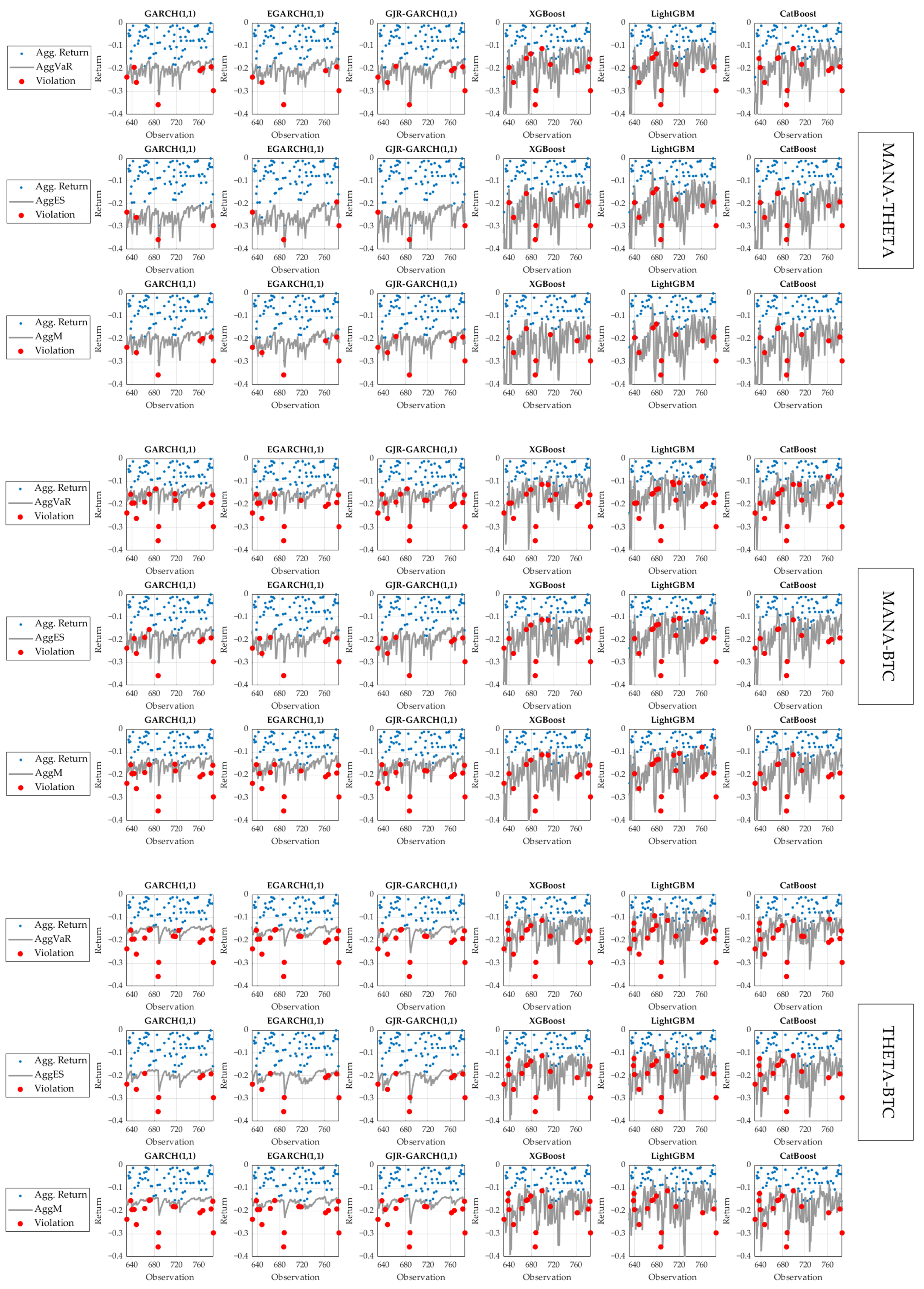
To quantify possible future losses resulting from aggregating the aforementioned cryptocurrencies, one needs to construct aggregate risk measures. These measures may include aggregate value-at-risk (AggVaR) and aggregate expected shortfall (AggES), which are basically the VaR and ES for an aggregate of returns at a given significance level over a specified time horizon. The former is determined based on the probability of the occurrence of the losses. The latter overcomes the former by accounting for the magnitude of all the losses exceeding the former. However, ES is sensitive to extreme losses, resulting in a risk forecast that may be too excessive, inaccurate, and not robust. This motivated Jadhav et al. (2009), Cont et al. (2010), and Josaphat and Syuhada (2021) to modify ES by truncating the losses beyond the VaR. This also led Zhang et al. (2014), Emmer et al. (2015), and Kratz et al. (2018) to approximate it using an average of VaRs at some significance levels based on the Riemann sum concept. Notwithstanding, these approaches removed information about extreme losses that may have important effects. Therefore, we proposed a convex combination of VaR and ES. In the context of aggregates or portfolios, we formulated a modified aggregate risk measure (AggM) by incorporating AggVaR and AggES with optimal weight. The idea behind employing AggM was to adjust the aggregate risk forecast by increasing the risk magnitude measured by AggVaR, while decreasing the risk magnitude measured by AggES such that the potential aggregate risk forecast was ideal. Using Syuhada’s (2020) coverage probability approach and Christoffersen’s (1998) backtesting technique, we needed to address the following question: Is AggM more accurate and more valid than AggVaR and AggES when quantifying the risk of the MANA–THETA, MANA–BTC, and THETA–BTC aggregates? Since AggM is a combination of AggVaR and AggES, it might have the advantages of both AggVaR and AggES. Accordingly, we hypothesized that the AggM for aggregates of the MANA–THETA, MANA–BTC, and THETA–BTC pairs would have higher forecast accuracy and validity than the respective AggVaR and AggES (H2).

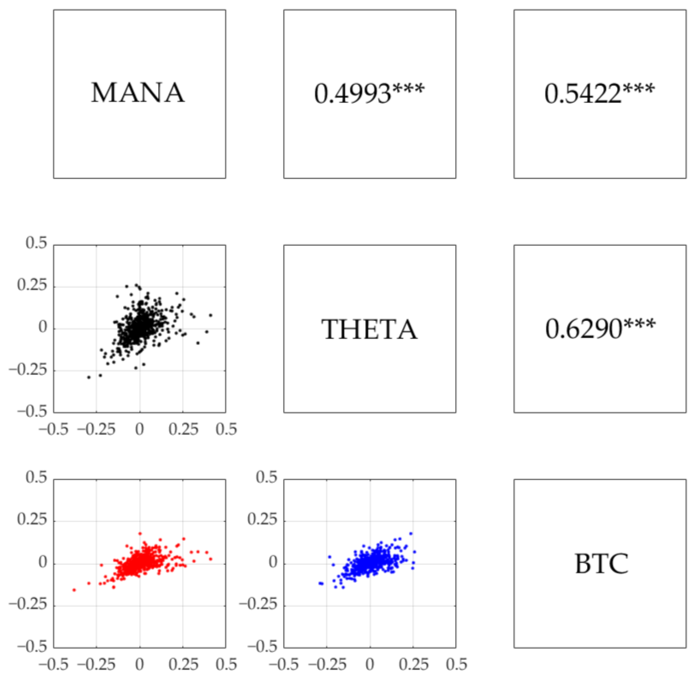
When computing the above aggregate risk measures, we had to account for the dependence between the returns of the above-mentioned cryptocurrencies. This study aimed to construct a dependent risk model for these cryptocurrencies through copulas. Copulas provide a way to model the dependence between two or more random variables (McNeil et al. 2015). Thus, we thought copulas might be useful to accommodate the dependence structure in each pair of these cryptocurrencies. Previous studies on cryptocurrencies have employed copulas to examine the best optimal portfolio (Boako et al. 2019), to determine a cryptocurrency able to maximize returns on investment (Tiwari et al. 2019), and to monitor the risk of various portfolios (Syuhada et al. 2022). In this paper, we employed copulas belonging to the Archimedean copula family: Clayton, Gumbel, and Frank. The Clayton (Gumbel) copula enabled us to handle lower (upper) tail dependence. Meanwhile, the Frank copula exhibiting lower and upper tail independence was taken into consideration as a benchmark. Employing Cramér–von Mises test, we attempted to address the following question: Are the lower tails of the MANA–THETA, MANA–BTC, and THETA–BTC pairs more dependent than their upper tails? We hypothesized that these pairs would tend to have lower tail dependence (H3).

In addition, we proposed the use of heteroskedastic models (HMs) as statistical tools to capture the stylized facts of the return and volatility of each cryptocurrency. The HMs chosen included generalized autoregressive conditional heteroskedastic (GARCH), exponential GARCH (EGARCH), and Glosten–Jagannathan–Runkle GARCH (GJR-GARCH) models. The GARCH model was first introduced by Engle (1982) and then perfected by Bollerslev (1986). Meanwhile, the EGARCH and GJR-GARCH models were the developments of the standard GARCH model. The former overcame the nonnegativity of the GARCH model’s constant and coefficient terms (Nelson 1991). Both of them allowed for leverage effects, i.e., the asymmetric responses of volatility to past negative and positive returns (Glosten et al. 1993; Nelson 1991). These HMs have been widely utilized for cryptocurrencies in the following instances: to forecast their volatility during bearish markets (Kyriazis et al 2019), to observe their skewed returns (Cerqueti et al 2020), to study common features of their returns (Fung et al. 2021), and to analyze asymmetry in their volatility (Apergis 2022; Wajdi et al. 2020). In addition to HMs, we considered other predictive models employing bagging and boosting methods, i.e., ensemble learning-based models (ELs), that can generate better generalization ability in time series forecasting (Khairalla 2022). More specifically, we selected three famous ELs to model the return and volatility of metaverse cryptocurrencies and Bitcoin. They included extreme gradient boosting (XGBoost), light gradient boosting machine (LightGBM), and categorical boosting (CatBoost). Many works have adopted these ELs, specifically for classification and regression tasks in engineering (Bo et al. 2022; Liu et al. 2022; Mahmood and Ali 2022) and medical science (Gao et al. 2020; Wang et al. 2022b). XGBoost performs risk assessment better than other machine learning models (Shi et al. 2022) and provides better accuracy than neural networks (Abdikan et al. 2022). It also provides stability and preciseness compared to the classical support vector model (Fan et al. 2018). Furthermore, XGBoost also provides the role of one of the comparable models with less time consumed (Dong et al. 2018). Meanwhile, LightGBM has better prediction results than k-nearest neighbors, decision trees, and random forest, specifically for corporate finance risk (Wang et al. 2022c). It also provides better accuracy in the stock selection model (Li et al. 2022) and outperforms the classical machine learning models (Ben Jabeur et al. 2021b; Laifa et al. 2021). CatBoost exhibits effective improvement compared to other advanced approaches (Ben Jabeur et al. 2021a), surpasses the accuracy of classical machine learning and artificial neural networks as a predictive model (Dutta and Roy 2022; Lu et al. 2022), and potentially increases accuracy as a hybrid model (Bileki et al. 2022). However, implementing ELs for cryptocurrencies is still scarce, especially to extract their return and volatility. Thus, we attempted to apply the aforementioned ELs to model the return and volatility of the metaverse cryptocurrencies and Bitcoin and address the following question: Do ELs perform better than HMs in forecasting the volatility and aggregate risk measures for the metaverse cryptocurrencies and Bitcoin? Based on their superior performance mentioned above, we hypothesized that ELs would produce volatility and aggregate risk measure forecasts with higher accuracy (H4).

The remainder of this paper is organized as follows. Section 2 describes the data, the models, and the way to construct AggVaR, AggES, and AggM through copulas. In the same section, we provide the coverage probability calculation and backtesting procedures to confirm that our aggregate risk measure forecasts are accurate and valid. Section 3 presents our findings and analyses regarding the modeling, forecasting, and validity. In Section 4, we then provide our concluding remarks.

2. Data and Methodology

This section discusses the datasets, the models, the aggregate risk measures, and the way to examine the accuracy and validity of their forecasts statistically.

2.1. Datasets

The daily price dataset for metaverse cryptocurrencies (i.e., Decentraland’s MANA and Theta Network’s THETA) and Bitcoin (BTC) was retrieved from CoinMarketCap.com (https://coinmarketcap.com, access on 20 May 2022), one of the cryptocurrency databases shown by Vidal-Tomás (2022b) to be an appropriate database for conducting an empirical cryptocurrency analysis. The data period started from 6 March 2020 to 30 April 2022. The training dataset used to estimate the model parameters took a ratio of 80% (628 observations). The remaining 20% data (157 observations) were used for testing and evaluation.

2.2. Dynamic Return Processes

The returns of the two metaverse cryptocurrencies and Bitcoin prices are defined as follows:

$$X_t=log\left({\displaystyle \frac{P_t^{\mathrm{M}}}{P_{t-1}^{\mathrm{M}}}}\right),Y_t=log\left({\displaystyle \frac{P_t^{\mathrm{T}}}{P_{t-1}^{\mathrm{T}}}}\right),Z_t=log\left({\displaystyle \frac{P_t^{\mathrm{B}}}{P_{t-1}^{\mathrm{B}}}}\right),$$

(1)

where $P_t^{\mathrm{M}}$, $P_t^{\mathrm{T}}$, and $P_t^{\mathrm{B}}$ denote the prices of MANA, THETA, and BTC at time t, respectively. We assumed that each of the return processes ${\left\{X_t\right\}}_{t\ge 0}$, ${\left\{Y_t\right\}}_{t\ge 0}$, and ${\left\{Z_t\right\}}_{t\ge 0}$ has a zero mean and follows a heteroskedastic model (see Section 2.3) due to the conditional heteroskedasticity property of the volatility. This process is also modeled through ensemble learning in Section 2.4.

2.3. Heteroskedastic Models

To model the return series in Equation (1), we utilized three heteroskedastic models (HMs). The first one was Bollerslev’s (1986) first-order generalized autoregressive conditional heteroskedastic or GARCH(1,1) model. More specifically, the GARCH(1,1) models for ${\left\{X_t\right\}}_{t\ge 0}$, ${\left\{Y_t\right\}}_{t\ge 0}$, and ${\left\{Z_t\right\}}_{t\ge 0}$ are given as follows:

$$\begin{array}{cc}\hfill X_t& ={\sigma }_{x,t}{\epsilon }_{x,t},{\sigma }_{x,t}^2=a_{0x}+a_{1x}{\sigma }_{x,t-1}^2+a_{2x}{X}_{t-1}^2,\hfill \end{array}$$

(2)

$$\begin{array}{cc}\hfill Y_t& ={\sigma }_{y,t}{\epsilon }_{y,t},{\sigma }_{y,t}^2=a_{0y}+a_{1y}{\sigma }_{y,t-1}^2+a_{2y}{Y}_{t-1}^2,\hfill \end{array}$$

(3)

$$\begin{array}{cc}\hfill Z_t& ={\sigma }_{z,t}{\epsilon }_{z,t},{\sigma }_{z,t}^2=a_{0z}+a_{1z}{\sigma }_{z,t-1}^2+a_{2z}{Z}_{t-1}^2,\hfill \end{array}$$

(4)

respectively, where $a_{0x},a_{0y},a_{0z}>0$ and $a_{jx},a_{jy},a_{jz}\ge 0$, for $j=1,2$. The restriction of these parameters, i.e., $a_{1x}+a_{2x}<1$, $a_{1y}+a_{2y}<1$, and $a_{1z}+a_{2z}<1$, is required to ensure the stationarity of the return process.

The second HM, used to model the returns, was the first-order exponential GARCH or EGARCH(1,1) model of Nelson (1991) that can be written as follows:

$$\begin{array}{cc}\hfill X_t& ={\sigma }_{x,t}{\epsilon }_{x,t},log\left({\sigma }_{x,t}^2\right)=b_{0x}+b_{1x}log\left({\sigma }_{x,t-1}^2\right)+b_{2x}\left({\displaystyle \frac{|X_{t-1}|}{{\sigma }_{x,t-1}}}-\sqrt{{\displaystyle \frac{2}{\mathsf{\pi }}}}\right)+b_{3x}\left({\displaystyle \frac{X_{t-1}}{{\sigma }_{x,t-1}}}\right),\hfill \end{array}$$

(5)

$$\begin{array}{cc}\hfill Y_t& ={\sigma }_{y,t}{\epsilon }_{y,t},log\left({\sigma }_{y,t}^2\right)=b_{0y}+b_{1y}log\left({\sigma }_{y,t-1}^2\right)+b_{2y}\left({\displaystyle \frac{|Y_{t-1}|}{{\sigma }_{y,t-1}}}-\sqrt{{\displaystyle \frac{2}{\mathsf{\pi }}}}\right)+b_{3y}\left({\displaystyle \frac{Y_{t-1}}{{\sigma }_{y,t-1}}}\right),\hfill \end{array}$$

(6)

$$\begin{array}{cc}\hfill Z_t& ={\sigma }_{z,t}{\epsilon }_{z,t},log\left({\sigma }_{z,t}^2\right)=b_{0z}+b_{1z}log\left({\sigma }_{z,t-1}^2\right)+b_{2z}\left({\displaystyle \frac{|Z_{t-1}|}{{\sigma }_{z,t-1}}}-\sqrt{{\displaystyle \frac{2}{\mathsf{\pi }}}}\right)+b_{3z}\left({\displaystyle \frac{Z_{t-1}}{{\sigma }_{z,t-1}}}\right),\hfill \end{array}$$

(7)

with $b_{jx},b_{jy},b_{jz}\in \mathbb{R}$, for $j=0,1,2,3$. The above models allow past negative and positive returns to have asymmetric impacts on the current volatility controlled by the parameter $b_{3·}$. More specifically, when $b_{3·}<0$, the impact of past negative returns ($b_{2·}-b_{3·}$) is higher than the impact of past positive returns ($b_{2·}+b_{3·}$). This is what we call the leverage effect. In contrast, the inverse leverage effect can be accommodated when $b_{3·}>0$, where the latter impact is larger than the former impact.

The last HM utilized to model the return series was a first-order Glosten–Jagannathan–Runkle GARCH or GJR-GARCH(1,1) model, proposed by Glosten et al. (1993). This model also permits us to capture the asymmetric volatility property determined by an indicator function; that is,1

$$\begin{array}{cc}\hfill X_t& ={\sigma }_{x,t}{\epsilon }_{x,t},{\sigma }_{x,t}^2=c_{0x}+c_{1x}{\sigma }_{x,t-1}^2+c_{2x}{X}_{t-1}^2+c_{3x}{X}_{t-1}^2{\mathbb{I}}_{(-\infty ,0)}\left(X_{t-1}\right),\hfill \end{array}$$

(8)

$$\begin{array}{cc}\hfill Y_t& ={\sigma }_{y,t}{\epsilon }_{y,t},{\sigma }_{y,t}^2=c_{0y}+c_{1y}{\sigma }_{y,t-1}^2+c_{2y}{Y}_{t-1}^2+c_{3y}{Y}_{t-1}^2{\mathbb{I}}_{(-\infty ,0)}\left(Y_{t-1}\right),\hfill \end{array}$$

(9)

$$\begin{array}{cc}\hfill Z_t& ={\sigma }_{z,t}{\epsilon }_{z,t},{\sigma }_{z,t}^2=c_{0z}+c_{1z}{\sigma }_{z,t-1}^2+c_{2z}{Z}_{t-1}^2+c_{3z}{Z}_{t-1}^2{\mathbb{I}}_{(-\infty ,0)}\left(Z_{t-1}\right).\hfill \end{array}$$

(10)

The restriction of the parameters is as follows: $c_{0x},c_{0y},c_{0z}>0$, $c_{jx},c_{jy},c_{jz}\ge 0$, for $j=1,2$, and $c_{3x},c_{3y},c_{3z}\in \mathbb{R}$, with $c_{1x}+\frac{1}{2}{c}_{3x}>0$, $c_{1y}+\frac{1}{2}{c}_{3y}>0$, $c_{1z}+\frac{1}{2}{c}_{3z}>0$, $c_{1x}+c_{2x}+\frac{1}{2}{c}_{3x}<1$, $c_{1y}+c_{2y}+\frac{1}{2}{c}_{3y}<1$, and $c_{1z}+c_{2z}+\frac{1}{2}{c}_{3z}<1$. If the leverage parameter $c_{3·}$ is positive (negative), the (inverse) leverage effect is allowed.

All the parameters of the GARCH(1,1), EGARCH(1,1), and GJR-GARCH(1,1) models are commonly estimated using the maximum likelihood method by assuming that each of the innovation processes ${\left\{{\epsilon }_{x,t}\right\}}_{t\ge 0}$, ${\left\{{\epsilon }_{y,t}\right\}}_{t\ge 0}$, and ${\left\{{\epsilon }_{z,t}\right\}}_{t\ge 0}$ is a standard Gaussian white noise with a distribution function $\Phi (·)$ and a probability function $\varphi (·)$. The maximized log-likelihood function can be employed to compare their goodness-of-fit performances.

2.4. Ensemble Learning-Based Models

For the comparisons, we also considered utilizing ensemble learning-based models (ELs) to model the return series of the metaverse cryptocurrencies and Bitcoin. Basically, ELs are multiple learning algorithms reconstructed through a statistical method, such as bootstrapping, bagging, and averaging. As mentioned in the Introduction section, we used three prominent ELs, including extreme gradient boosting (XGBoost), light gradient boosting machine (LightGBM), and categorical boosting (CatBoost). The standard algorithms for these ELs are provided in

Table 1. XGBoost algorithm (Chen and Guestrin 2016; Mushava 2022).

Stage
Input	1. Training set consisting of predictors $\mathbf{x}={\left(x_i\right)}_{i=1}^n$ and responses $\mathbf{y}={\left(y_i\right)}_{i=1}^n$.
	2. Differentiable loss function $\mathcal{L}(\mathbf{y},f(\mathbf{x}\left)\right)$.
	3. K number of weak learners.
	4. Learning rate $r\in (0,1)$.
Process	1. Model initialization with a constant value:
	${\displaystyle {\widehat{f}}^{\left(0\right)}\left(\mathbf{x}\right)=\underset{\theta }{\arg \min }\sum _{i=1}^n\mathcal{L}(y_i,\theta )}$.
	2. for k = 1 to K do
	a. Compute the Gradient:
	${\left.{\widehat{G}}_k={\displaystyle \frac{\partial \mathcal{L}(\mathbf{y},f(\mathbf{x}\left)\right)}{\partial f\left(\mathbf{x}\right)}}\right|}_{f\left(x\right)={\widehat{f}}^{(k-1)}\left(\mathbf{x}\right)}$
	b. Compute the Hessian:
	${\left.{\widehat{H}}_k={\displaystyle \frac{{\partial }^2\mathcal{L}(\mathbf{y},f\left(\mathbf{x}\right))}{\partial f{\left(\mathbf{x}\right)}^2}}\right|}_{f\left(x\right)={\widehat{f}}^{(k-1)}\left(\mathbf{x}\right)}$
	c. Solve the optimization:
	${\displaystyle {\widehat{\phi }}_k=\underset{\phi \in \Phi }{\arg \min }\sum _{i=1}^n{\displaystyle \frac{1}{2}}{\widehat{H}}_k{\left[-{\displaystyle \frac{{\widehat{G}}_k}{{\widehat{H}}_k}}-\phi \left(x_i\right)\right]}^2}$
	${\widehat{f}}_k\left(\mathbf{x}\right)=r{\widehat{\phi }}_k\left(\mathbf{x}\right)$
	d. Update:
	${\widehat{f}}^{\left(k\right)}\left(\mathbf{x}\right)={\widehat{f}}^{(k-1)}\left(\mathbf{x}\right)+{\widehat{f}}_k\left(\mathbf{x}\right)$.
Output	${\displaystyle {\widehat{f}}_{\mathrm{XGBoost}}\left(\mathbf{x}\right)={\widehat{f}}^{\left(K\right)}\left(\mathbf{x}\right)=\sum _{k=0}^K{\widehat{f}}^{\left(k\right)}\left(\mathbf{x}\right)}$.

,

Table 2. LightGBM algorithm (Ke et al. 2017; Li et al. 2021).

Stage
Input	1. Training set consisting of predictors $\mathbf{x}={\left(x_i\right)}_{i=1}^n$ and responses $\mathbf{y}={\left(y_i\right)}_{i=1}^n$.
	2. Differentiable loss function $\mathcal{L}(\mathbf{y},f(\mathbf{x}\left)\right)$.
	3. K number of basic classifiers.
	4. Constant $\lambda ,\gamma \in (0,1)$.
	5. T number of leaf nodes.
	6. Random weights of node ${\omega }_0={\left({\omega }_j^{\left(0\right)}\right)}_{j=1}^T$.
Process	1. Model initialization with a constant value:
	${\displaystyle {\widehat{f}}^{\left(0\right)}\left(\mathbf{x}\right)=\underset{\theta }{\arg \min }\sum _{i=1}^n\mathcal{L}(y_i,\theta )}$.
	2. for $k=1$ to K do
	a. Find ${\phi }_k$ by solving the optimization:
	${\displaystyle {\phi }_k=\underset{\phi \in \mathsf{\Phi }}{\arg \min }\sum _{i=1}^n\mathcal{L}\left(y_i,f^{(k-1)}\left(x_i\right)+\phi \left(x_i\right)\right)}$.
	b. Compute:
	$g_i={\displaystyle \frac{\partial \mathcal{L}(y_i,f\left(x_i\right))}{\partial f\left(x_i\right)}}$.
	$h_i={\displaystyle \frac{{\partial }^2\mathcal{L}(y_i,f\left(x_i\right))}{\partial f{\left(x_i\right)}^2}}$.
	c. Calculate:
	$J_i=\mathcal{L}\left(y_i,f^{(k-1)}\left(x_i\right)\right)+g_i{\phi }_k\left(x_i\right)+{\displaystyle \frac{1}{2}}{h}_i{\phi }_k^2\left(x_i\right)$.
	${\displaystyle \mathsf{\Omega }\left({\phi }_k\right)=\gamma T+{\displaystyle \frac{1}{2}}\lambda \sum _{j=1}^T{\left({\omega }_j^{\left(k\right)}\right)}^2}$.
	${\displaystyle f^{\left(k\right)}\left(\mathbf{x}\right)=\mathsf{\Omega }\left({\phi }_k\right)+\sum _{i=1}^n{J}_i}$.
	d. Update the weights of node:
	${\omega }_j^{(k+1)}={\omega }_j^{\left(k\right)}-{\displaystyle \frac{{\sum }_{i\in I}{g}_i}{\lambda +{\sum }_{i\in I}{h}_i}}$.
Output	${\displaystyle {\widehat{f}}_{\mathrm{LighGBM}}\left(\mathbf{x}\right)={\widehat{f}}^{\left(K\right)}\left(\mathbf{x}\right)=\sum _{k=0}^K{\widehat{f}}^{\left(k\right)}\left(\mathbf{x}\right)}$.

and

Table 3. CatBoost algorithm (Prokhorenkova et al. 2018).

Stage
Input	1. Training set consisting of predictors $\mathbf{x}={\left(x_i\right)}_{i=1}^n$ and responses $\mathbf{y}={\left(y_i\right)}_{i=1}^n$.
	2. Maximum iteration, I.
	3. Learning rate $\gamma \in (0,1)$.
	4. Loss function $\mathcal{L}$ with type Mode.
	5. ${\left\{{\sigma }_i\right\}}_{i=1}^s$.
Preprocess	1. $\sigma =$ random permutation of $[1,n]$.
	2. $M_i=0$ for $i=1,2,\dots ,n$.
	3. for $t=1$ to I do
	a. Calculate:
	$r_i=y_i-M_{\sigma \left(i\right)-1}\left(x_i\right)$, for $i=1,2,\dots ,n$.
	b. Compute:
	$\Delta M_i=$ LearnModel$((x_j,r_j):\sigma \left(j\right)\le i)$, for $i=1,\dots ,n$.
	$M_i=M_i+\Delta M_i$, for $i=1,2,\dots ,n$.
Process
Output	Set of values, M, and decision tree T.

.

2.5. Copulas

We assumed that cryptocurrency returns are dependent. We modeled their dependence using the so-called copula. A d-dimensional copula is a joint distribution function for random variables $U_1,\dots ,U_d$ uniformly distributed on a unit hypercube ${[0,1]}^d$(McNeil et al. 2015). This means that a copula C is a mapping of ${[0,1]}^d$ into $[0,1]$, i.e., $C:{[0,1]}^d\to [0,1]$, with $C\left(\mathbf{u}\right)=C(u_1,\dots ,u_d)=\mathbb{P}(U_1\le u_1,\dots ,U_d\le u_d)$ for all $\mathbf{u}\in {[0,1]}^d$. There are three properties that must hold (McNeil et al. 2015):

• $C(u_1,\dots ,u_d)=0$ if $u_i=0$ for any i.
• $C(1,\dots ,1,u_i,1,\dots ,1)=u_i$ for all $i\in \{1,\dots ,d\}$ and $u_i\in [0,1]$.
• For all $(a_1,\dots ,a_d),(b_1,\dots ,b_d)\in {[0,1]}^d$ with $a_i\le b_i$, we have

  $$\sum _{i_1=1}^2\dots \sum _{i_d=1}^2{(-1)}^{i_1+\dots +i_d}C(u_{1i_1},\dots ,u_{d{i}_d})\ge 0,$$

  where $u_{j1}=a_j$ and $u_{j2}=b_j$ for all $j\in \left\{1,\dots ,d\right\}$.

The existence of a copula C for any multivariate distribution function F is guaranteed by Sklar’s theorem, allowing us to express it as follows:

$$F\left(\mathbf{x}\right)=F(x_1,\dots ,x_d)=C\left[F_1\left(x_1\right),\dots ,F_d\left(x_d\right)\right],\mathbf{x}\in {\mathbb{R}}^d,$$

where $F_1,\dots ,F_d$ are marginal distribution functions.

In this study, we considered $d=2$, since we attempted to model the dependence structure in each pair of two cryptocurrencies. To do a limitation, we only fitted three copulas from the Archimedean copula family described in the following:

• Clayton Copula

  $$C^{\mathrm{Cl}}(u,v;\theta )={(u^{-\theta }+v^{-\theta }-1)}^{-1/\theta }$$

  (11)

  where $\theta \in (0,\infty )$.
• Gumbel Copula

  $$C^{\mathrm{Gu}}(u,v;\theta )=exp\left\{-{\left[{(-ln\left(u\right))}^{\theta }+{(-ln\left(v\right))}^{\theta }\right]}^{1/\theta }\right\}$$

  (12)

  where $\theta \in [1,\infty )$.
• Frank Copula

  $$C^{\mathrm{Fr}}(u,v;\theta )=-{\displaystyle \frac{1}{\theta }}ln\left[1+{\displaystyle \frac{(e^{-\theta u}-1)(e^{-\theta v}-1)}{e^{-\theta }-1}}\right]$$

  (13)

  where $\theta \in \mathbb{R}\backslash \left\{0\right\}$.

The plot of their copula density $c(u,v;\theta )={\partial }^{2}C(u,v;\theta )/\partial u\partial v$ is provided in Figure 1, demonstrating that the Clayton (Gumbel) copula exhibited lower (upper) tail dependence, and the Frank copula had tail independence. Suppose that two random variables X and Y had marginal distribution functions $F_X$ and $F_Y$ and a joint distribution function determined by these copulas. In that case, we could compute their Pearson’s correlation coefficient $\rho$ using the following equation (Schweizer and Wolff 1981; Syuhada and Hakim 2020):

$$\begin{array}{c}\hfill \rho ={\displaystyle \frac{{\displaystyle {\int \int }_{{[0,1]}^2}\left[C(u,v;\theta )-uv\right]\mathrm{d}{F}_X^{-1}\left(u\right)\mathrm{d}{F}_Y^{-1}\left(v\right)}}{\sqrt{\mathrm{Var}\left(X\right)}\sqrt{\mathrm{Var}\left(Y\right)}}}.\end{array}$$

(14)

In this study, the copula parameter $\theta$ was estimated using the maximum likelihood method, and the goodness of copula fitting was evaluated using the Cramér–von Mises test. More specifically, this hypothesis test was utilized to examine whether the copula fitting was statistically adequate (Genest et al. 2006).

2.6. Aggregate Risk Measures

Aggregating individual risks is expected to create a low value with high accuracy instead of simply summing them up (Syuhada and Hakim 2020). This reason urged us to formulate risk measures for an aggregate of future risks or returns at time $t+1$, given ${\mathcal{F}}_t$ denoting a set of information available at time t. In this study, we attempted to forecast the risk measures for three aggregates, including $X_{t+1}+Y_{t+1}$, $X_{t+1}+Z_{t+1}$, and $Y_{t+1}+Z_{t+1}$, by using three aggregate risk measures described as follows:

• Aggregate Value-at-Risk (AggVaR)
  The first risk measure was aggregate value-at-risk (AggVaR), the VaR for an aggregate of returns. We linked these returns through a copula and derived its formula by using the variance–covariance principle with zero-mean assumptions $\mathbb{E}\left(X_{t+1}\right|{\mathcal{F}}_t)=\mathbb{E}\left(Y_{t+1}\right|{\mathcal{F}}_t)=\mathbb{E}\left(Z_{t+1}\right|{\mathcal{F}}_t)=0$. Note that the VaR for the return $X_{t+1}$ at a given significance level $\alpha \in (0,1)$ is given by ${\mathrm{VaR}}_{x,t+1}^{\alpha }={\Phi }^{-1}\left(\alpha \right)\sqrt{\mathrm{Var}\left(X_{t+1}|{\mathcal{F}}_t\right)}$. For the case of $X_{t+1}+Y_{t+1}$, we can, thus, obtain its AggVaR as follows:

  $${\mathrm{AggVaR}}_{x+y,t+1}^{\alpha }={\Phi }^{-1}\left(\alpha \right)\sqrt{\mathrm{Var}\left(X_{t+1}+Y_{t+1}|{\mathcal{F}}_t\right)},$$

  (15)

  where

  $$\begin{array}{cc}\hfill & \mathrm{Var}\left(X_{t+1}+Y_{t+1}|{\mathcal{F}}_t\right)\hfill \\ \hfill & =\mathrm{Var}\left(X_{t+1}|{\mathcal{F}}_t\right)+\mathrm{Var}\left(Y_{t+1}|{\mathcal{F}}_t\right)+2{\rho }_{x,y}\sqrt{\mathrm{Var}\left(X_{t+1}|{\mathcal{F}}_t\right)\mathrm{Var}\left(Y_{t+1}|{\mathcal{F}}_t\right)}\hfill \\ \hfill & ={\sigma }_{x,t+1}^2+{\sigma }_{y,t+1}^2+2{\rho }_{x,y}{\sigma }_{x,t+1}{\sigma }_{y,t+1},\hfill \end{array}$$

  (16)

  with

  $$\begin{array}{cc}\hfill {\rho }_{x,y}& =\mathrm{Corr}(X_{t+1},Y_{t+1}|{\mathcal{F}}_t)\hfill \\ \hfill & =\mathrm{Corr}({\epsilon }_{x,t+1},{\epsilon }_{y,t+1})\hfill \\ \hfill & ={\int \int }_{{[0,1]}^2}\left[C(u,v;{\theta }_{x,y})-uv\right]\mathrm{d}{\Phi }^{-1}\left(u\right)\mathrm{d}{\Phi }^{-1}\left(v\right)\hfill \\ \hfill & ={\int \int }_{{[0,1]}^2}\left[C(u,v;{\theta }_{x,y})-uv\right]{\displaystyle \frac{1}{\varphi \left[{\Phi }^{-1}\left(u\right)\right]}}{\displaystyle \frac{1}{\varphi \left[{\Phi }^{-1}\left(v\right)\right]}}\mathrm{d}u\mathrm{d}v.\hfill \end{array}$$

  (17)
  Similarly, we formulate the AggVaR for $X_{t+1}+Z_{t+1}$ and the AggVaR for $Y_{t+1}+Z_{t+1}$ as follows:

  $$\begin{array}{cc}\hfill {\mathrm{AggVaR}}_{x+z,t+1}^{\alpha }& ={\Phi }^{-1}\left(\alpha \right)\sqrt{{\sigma }_{x,t+1}^2+{\sigma }_{z,t+1}^2+2{\rho }_{x,z}{\sigma }_{x,t+1}{\sigma }_{z,t+1}},\hfill \end{array}$$

  (18)

  $$\begin{array}{cc}\hfill {\mathrm{AggVaR}}_{y+z,t+1}^{\alpha }& ={\Phi }^{-1}\left(\alpha \right)\sqrt{{\sigma }_{y,t+1}^2+{\sigma }_{z,t+1}^2+2{\rho }_{y,z}{\sigma }_{y,t+1}{\sigma }_{z,t+1}},\hfill \end{array}$$

  (19)

  respectively.
• Aggregate Expected Shortfall (AggES)
  The second risk measure was aggregate expected shortfall (AggES), the ES for an aggregate of returns. We adopted a simple ES under the normality assumption to construct this risk measure. Note that the ES for the return $X_{t+1}$ is given as follows:

  $$\begin{array}{cc}\hfill {\mathrm{ES}}_{x,t+1}^{\alpha }& =\mathbb{E}\left(X_{t+1}|X_{t+1}\le {\mathrm{VaR}}_{x,t+1}^{\alpha },{\mathcal{F}}_t\right)\hfill \\ \hfill & ={\displaystyle \frac{1}{\alpha }}{\int }_0^{\alpha }{\mathrm{VaR}}_{x,t+1}^u\mathrm{d}u\hfill \\ \hfill & ={\displaystyle \frac{\sqrt{\mathrm{Var}\left(X_{t+1}|{\mathcal{F}}_t\right)}}{\alpha }}{\int }_0^{\alpha }{\Phi }^{-1}\left(u\right)\mathrm{d}u\hfill \\ \hfill & =-{\displaystyle \frac{\varphi \left[{\Phi }^{-1}\left(\alpha \right)\right]}{\alpha }}\sqrt{\mathrm{Var}\left(X_{t+1}|{\mathcal{F}}_t\right)}.\hfill \end{array}$$
  By adopting this result, we could obtain the AggES for $X_{t+1}+Y_{t+1}$, the AggES for $X_{t+1}+Z_{t+1}$, and the AggES for $Y_{t+1}+Z_{t+1}$ as follows:

  $$\begin{array}{cc}\hfill {\mathrm{AggES}}_{x+y,t+1}^{\alpha }& =-{\displaystyle \frac{\varphi \left[{\Phi }^{-1}\left(\alpha \right)\right]}{\alpha }}\sqrt{{\sigma }_{x,t+1}^2+{\sigma }_{y,t+1}^2+2{\rho }_{x,y}{\sigma }_{x,t+1}{\sigma }_{y,t+1}},\hfill \end{array}$$

  (20)

  $$\begin{array}{cc}\hfill {\mathrm{AggES}}_{x+z,t+1}^{\alpha }& =-{\displaystyle \frac{\varphi \left[{\Phi }^{-1}\left(\alpha \right)\right]}{\alpha }}\sqrt{{\sigma }_{x,t+1}^2+{\sigma }_{z,t+1}^2+2{\rho }_{x,z}{\sigma }_{x,t+1}{\sigma }_{z,t+1}},\hfill \end{array}$$

  (21)

  $$\begin{array}{cc}\hfill {\mathrm{AggES}}_{y+z,t+1}^{\alpha }& =-{\displaystyle \frac{\varphi \left[{\Phi }^{-1}\left(\alpha \right)\right]}{\alpha }}\sqrt{{\sigma }_{y,t+1}^2+{\sigma }_{z,t+1}^2+2{\rho }_{y,z}{\sigma }_{y,t+1}{\sigma }_{z,t+1}},\hfill \end{array}$$

  (22)

  respectively.
• Modified Aggregate Risk Measure (AggM)
  The last risk measure was a convex combination of AggVaR and AggES called modified aggregate risk measure (AggM). The AggM for the three aggregates is expressed as follows:

  $$\begin{array}{cc}\hfill {\mathrm{AggM}}_{x+y,t+1}^{\alpha }& ={\omega }_{x,y}{\mathrm{AggVaR}}_{x+y,t+1}^{\alpha }+(1-{\omega }_{x,y}){\mathrm{AggES}}_{x+y,t+1}^{\alpha },\hfill \end{array}$$

  (23)

  $$\begin{array}{cc}\hfill {\mathrm{AggM}}_{x+z,t+1}^{\alpha }& ={\omega }_{x,z}{\mathrm{AggVaR}}_{x+z,t+1}^{\alpha }+(1-{\omega }_{x,z}){\mathrm{AggES}}_{x+z,t+1}^{\alpha },\hfill \end{array}$$

  (24)

  $$\begin{array}{cc}\hfill {\mathrm{AggM}}_{y+z,t+1}^{\alpha }& ={\omega }_{y,z}{\mathrm{AggVaR}}_{y+z,t+1}^{\alpha }+(1-{\omega }_{y,z}){\mathrm{AggES}}_{y+z,t+1}^{\alpha },\hfill \end{array}$$

  (25)

  with ${\omega }_{x,y},{\omega }_{x,z},{\omega }_{y,z}\in (0,1)$ denoting optimal weights determined by applying a simple adaptive random search algorithm on the training dataset. As we know, (Agg)ES quantifies losses beyond (Agg)VaR, implying that (Agg)VaR is an essential infimum of loss (Cascos and Molchanov 2013; Rohmawati and Syuhada 2015). The idea of using AggM was to increase the risk magnitude measured by AggVaR while decreasing the risk magnitude measured by AggES, resulting in an optimal risk magnitude.

2.7. Coverage Probability

The value of the risk measure forecast shows the possible future loss of a specific asset at a certain level of significance. Based on this fact, we had an important question concerning how accurate our risk measure forecasts were. To ensure that the risk measure forecasts were accurate, the role of coverage probability was required (Syuhada 2020). Suppose that $\widehat{\mathrm{RiskM}}{}_{s,t+1}^{\alpha }$ denotes the forecast for an aggregate risk measure (i.e., either AggVaR, AggES, or AggM) at time $t+1$ with a significance level $\alpha$. In that case, its accuracy could be evaluated by calculating its coverage probability as follows (Syuhada 2020):

$$\mathbb{P}\left(S_{t+1}\le \widehat{\mathrm{RiskM}}{}_{s,t+1}^{\alpha }|{\mathcal{F}}_t\right)=\mathbb{E}\left[F_{S_{t+1}|{\mathcal{F}}_t}\left(\widehat{\mathrm{RiskM}}{}_{s,t+1}^{\alpha }\right)|{\mathcal{F}}_t\right],$$

(26)

where $S_{t+1}$ is equal to either $X_{t+1}+Y_{t+1}$, $X_{t+1}+Z_{t+1}$, or $Y_{t+1}+Z_{t+1}$. For the case of AggES, the coverage probability was calculated by finding the value of $\alpha$ in Equation (22).

2.8. Backtesting Methods

It was also important to examine whether the resulting risk measure forecast was valid. To do so, Christoffersen’s (1998) backtesting technique was employed. The procedure starts by defining a binary sequence of violations in our simulation for each aggregate dataset $\left\{S_{t+1}\right\}$. We denote it by $\left\{I_{t+1}\right\}$, with

$$I_{t+1}=\left\{\begin{array}{cc}0,\hfill & S_{t+1}>\widehat{\mathrm{RiskM}}{}_{s,t+1}^{\alpha },\hfill \\ 1,\hfill & S_{t+1}\le \widehat{\mathrm{RiskM}}{}_{s,t+1}^{\alpha }.\hfill \end{array}\right.$$

(27)

Christoffersen’s test aims to evaluate the null hypothesis

$$H_0:I_{t+1}\sim \mathrm{Bernoulli}\left(\alpha \right)(\mathrm{i}.\mathrm{i}.\mathrm{d}.).$$

(28)

This sequence must satisfy unconditional coverage and independence properties to ensure that the risk forecast is valid (Christoffersen 1998). Thus, to evaluate the above null hypothesis, we required two test statistics in the form of the likelihood ratio (LR) that must be computed. First, the test statistic for Christoffersen’s unconditional coverage is given as follows:

$${\mathrm{LR}}_{\mathrm{uc}}=-2log\left[{\left({\displaystyle \frac{1-\alpha }{1-\pi }}\right)}^{n_0}{\left({\displaystyle \frac{\alpha }{\pi }}\right)}^{n_1}\right],$$

(29)

where $n_0$ and $n_1$ denote the number of “0” and “1” in $\left\{I_{t+1}\right\}$, respectively, and $\pi =n_1/(n_0+n_1)$. The second test statistic is the likelihood ratio for the independence test. The test statistic for Christoffersen’s independence test is formulated as follows:

$${\mathrm{LR}}_{\mathrm{ind}}=-2log\left({\displaystyle \frac{L_2}{L_1}}\right),$$

(30)

where $L_1={(1-{\pi }_{01})}^{n_{00}}{\pi }_{01}^{n_{01}}{(1-{\pi }_{11})}^{n_{10}}{\pi }_{11}^{n_{11}}$, $L_2={(1-\pi )}^{(n_{00}+n_{10})}{\pi }^{(n_{01}+n_{11})}$, ${\pi }_{01}=n_{01}/(n_{00}+n_{01})$, and ${\pi }_{11}=n_{11}/(n_{10}+n_{11})$, with $n_{ij}$ denoting the number of the term i followed by the term j in $\left\{I_{t+1}\right\}$. In summary, the test statistic for Christoffersen’s test is the summation of the statistics ${\mathrm{LR}}_{\mathrm{uc}}$ and ${\mathrm{LR}}_{\mathrm{ind}}$; that is,

$${\mathrm{LR}}_{\mathrm{cc}}={\mathrm{LR}}_{\mathrm{uc}}+{\mathrm{LR}}_{\mathrm{ind}}.$$

(31)

This ${\mathrm{LR}}_{\mathrm{cc}}$ asymptotically follows a chi-square distribution with two degrees of freedom. If the resulting p-value is less than the considered significance level ($\alpha$) of the test, then the null hypothesis stated in Equation (28) is rejected.

3. Empirical Findings

3.1. Data Visualization and Preliminary Analysis

We depict in Figure 2 the dynamic of the daily prices and returns of MANA, THETA, and BTC from 6 March 2020 to 30 April 2022. From this figure, we observed a tendency for the prices of all the cryptocurrencies to be dependent. More specifically, a peak occurred in the four hundredth observation, and after the six hundredth observation, all the prices gradually decreased. This fact signified that these three cryptocurrencies were likely dependent on each other. Figure 2 also shows that MANA and THETA returns were relatively higher in value and more volatile than BTC returns. This evidence was confirmed by their summary statistics, reported in

Table 4. Summary statistics of metaverse cryptocurrencies and Bitcoin returns.

Statistic	MANA	THETA	BTC
Mean	0.0043	0.0036	0.0018
Standard Deviation	0.0860	0.0767	0.0419
Skewness	1.5330	−1.0949	−2.0434
Kurtosis	25.1130	9.5274	29.1885
ADF (p-Value)	−8.9563 ** (0.0100)	−8.8064 ** (0.0100)	−9.3992 ** (0.0100)
Ljung–Box (p-Value)	22.8975 (0.2939)	42.2619 *** (0.0026)	32.4647 ** (0.0386)
ARCH (p-Value)	34.4689 *** (0.0000)	6.9104 *** (0.0085)	3.7134 * (0.0539)

The asterisks *, **, and *** indicate statistical significance at the 10%, 5%, and 1% levels, respectively.

, where the means (respectively, standard deviations) of MANA and THETA returns were two times higher than the mean (respectively, standard deviation) of BTC returns. This suggested that the two metaverse cryptocurrencies provided higher returns for investors, but were riskier than BTC, in line with what Yousaf and Yarovaya (2022a) concluded from their study. This was also preliminary support for our first hypothesis (H1) that they had a higher risk than BTC.

We also observe from Table 4 that the metaverse cryptocurrencies and BTC return series were stationary processes with a weak serial correlation, based on the augmented Dickey–Fuller (ADF) and Ljung–Box tests. Engle’s (1982) ARCH test confirmed that they possessed a conditional heteroskedasticity effect, leading us to make use of GARCH-type specifications to model the return and volatility. Surprisingly, the ARCH test statistic for MANA and THETA returns was higher than that for BTC returns, indicating that the former’s heteroskedasticity effect was stronger than the latter’s heteroskedasticity effect. In addition, the scatter and correlation plots for the MANA–THETA, MANA–BTC, and THETA–BTC return pairs in Figure 3 highlighted that they were highly correlated, which was statistically significant at the 1% level. Figure 3 also shows that the correlation between MANA and THETA (0.4993) was weaker than the MANA–BTC correlation (0.5422) and THETA–BTC correlation (0.6290). This suggested that a portfolio made up of the two metaverse cryptocurrencies might provide a higher diversification benefit for investors. Interestingly, the three pairs (i.e., MANA–THETA, MANA–BTC, and THETA–BTC) exhibited lower tail dependence, indicating that their extreme negative returns tended to co-move in the same direction, as we hypothesized (H3) in the Introduction section. This inspired us to employ a dependence model, determined using a copula (in particular, a Clayton copula).

For further analyses, our dataset was split into a training set (80%) and a testing set (20%). The training set was used to estimate the marginal model parameter, model the dependence through copulas, and extract the optimal weight for the AggM risk measure forecasting. Afterward, the testing set was employed to assess and compare our models’ volatility and risk measure forecasting performances.

3.2. Return and Volatility Modeling Using Heteroskedastic Models and Ensemble Learning

We first considered that the return process of each cryptocurrency followed first-order GARCH, EGARCH, and GJR-GARCH marginal models under the normality assumption for each innovation, as formulated in Equations (2)–(10). We used the maximum simulated likelihood method to estimate their parameters. We present in

Table 5. Parameter estimation result for heteroskedastic models.

		MANA	THETA	BTC
GARCH(1,1)	${\widehat{a}}_0$ (Std. Error)	0.0011 *** (0.0001)	0.0007 *** (0.0002)	0.0000 *** (0.0000)
	${\widehat{a}}_1$ (Std. Error)	0.5205 *** (0.0274)	0.7837 *** (0.0448)	0.9276 *** (0.0145)
	${\widehat{a}}_2$ (Std. Error)	0.4336 *** (0.0495)	0.1085 *** (0.0181)	0.0469 *** (0.0107)
	Log-L	718.49	711.19	1102.22
EGARCH(1,1)	${\widehat{b}}_0$ (Std. Error)	−0.9094 *** (0.1093)	−0.4542 *** (0.1618)	−0.2534*** (0.0701)
	${\widehat{b}}_1$ (Std. Error)	0.8105 *** (0.0224)	0.9079 *** (0.9079)	0.9586 *** (0.0112)
	${\widehat{b}}_2$ (Std. Error)	0.5916 *** (0.0555)	0.2092 *** (0.0298)	0.1052 *** (0.0239)
	${\widehat{b}}_3$ (Std. Error)	0.0017 (0.0331)	−0.0278 ** (0.0141)	−0.0646 *** (0.0103)
	Log-L	722.41	712.03	1110.31
GJR-GARCH(1,1)	${\widehat{c}}_0$ (Std. Error)	0.0010 *** (0.0001)	0.0008 *** (0.0002)	0.0001 *** (0.0000)
	${\widehat{c}}_1$ (Std. Error)	0.5134 *** (0.0443)	0.7713 *** (0.0401)	0.8712 *** (0.0231)
	${\widehat{c}}_2$ (Std. Error)	0.3746 *** (0.0414)	0.0886 *** (0.0229)	0.0241 (0.0179)
	${\widehat{c}}_3$ (Std. Error)	0.0221 * (0.1209)	0.0646 ** (0.0268)	0.1208 *** (0.0000)
	Log-L	720.03	712.37	1106.21

The asterisks *, **, and *** indicate statistical significance at the 10%, 5%, and 1% levels, respectively. Log-L stands for the maximized log-likelihood value. The highest Log-L for each cryptocurrency is presented in boldface.

the resulting parameter estimates and the maximized log-likelihood value (Log-L) for each heteroskedastic model (HM). These estimation results showed that the HMs were suitable models for the return and volatility of each cryptocurrency, the parameter estimates of which were statistically significant and satisfied the stationary conditions given in Section 2.3. We also found that the EGARCH(1,1) model exhibited the (second) highest Log-L when modeling MANA and BTC (THETA) returns and volatilities, meaning that it tended to be the best-fitting HM. On the other hand, the GJR–GARCH(1,1) model had the (second) highest Log-L when modeling THETA (MANA and BTC) returns and volatilities, indicating that it ranked second as the best-fitting HM. Surprisingly, all the HMs worked best on BTC with the highest Log-L and had parameter estimates with the lowest standard error among others. This might be because of the least volatile movement of its return series.

The modeling, based on the ELs, was carried out using Python programming (v3.7.6) with specific libraries (i.e., xgboost v1.2.1, lightgbm v3.1.0, and catboost v0.24.3). We did not tune the parameter; we, instead, used the default parameter built in each library. To ensure that our results, based on the HMs and ELs, were comparable, we proposed the use of root mean squared error (RMSE), weighted mean absolute percentage error (WMAPE), and quasi-likelihood (QLIKE) to measure the accuracy of the volatility forecasts. These measures were defined using the testing dataset as follows:

$$\begin{array}{cc}\hfill \mathrm{RMSE}& =\sqrt{{\displaystyle \frac{1}{T}}\sum _{t=1}^T{\left({\widehat{\sigma }}_{·,N+t}^2-{\tilde{\sigma }}_{·,N+t}^2\right)}^2},\hfill \\ \hfill \mathrm{WMAPE}& ={\displaystyle \frac{{\sum }_{t=1}^T\left|{\widehat{\sigma }}_{·,N+t}^2-{\tilde{\sigma }}_{·,N+t}^2\right|}{{\sum }_{t=1}^T{\tilde{\sigma }}_{·,N+t}^2}},\hfill \\ \hfill \mathrm{QLIKE}& ={\displaystyle \frac{1}{T}}\sum _{t=1}^T\left[log\left({\widehat{\sigma }}_{·,N+t}^2\right)+{\displaystyle \frac{{\tilde{\sigma }}_{·,N+t}^2}{{\widehat{\sigma }}_{·,N+t}^2}}\right],\hfill \end{array}$$

where ${\tilde{\sigma }}_{·,N+t}^2$ is the volatility proxy, and N and T are the size of the training and testing datasets, respectively. In particular, we considered ${\tilde{\sigma }}_{x,N+t}^2=X_{N+t}^2$ for the case of MANA, ${\tilde{\sigma }}_{y,N+t}^2=Y_{N+t}^2$ for the case of THETA, and ${\tilde{\sigma }}_{z,N+t}^2=Z_{N+t}^2$ for the case of BTC, which were realized volatilities. The use of WMAPE and QLIKE avoids the possibility of zero division. The resulting volatility forecasts are depicted in Figure 4, and the forecast accuracy evaluation is given in

Table 6. Volatility forecast accuracy.

	MANA			THETA			BTC
	RMSE	WMAPE	QLIKE	RMSE	WMAPE	QLIKE	RMSE	WMAPE	QLIKE
GARCH(1,1)	0.0034	0.7005	22.5182	0.0027	0.6778	21.8645	0.0010	0.6438	34.7203
EGARCH(1,1)	0.0035	0.7542	22.3657	0.0028	0.7266	21.7566	0.0011	0.7717	33.8823
GJR-GARCH(1,1)	0.0037	0.7547	22.4564	0.0028	0.7170	21.7919	0.0010	0.7450	34.1062
XGBoost	0.0036	0.5779	36.5278	0.0030	0.5803	30.5082	0.0010	0.5864	34.7294
LightGBM	0.0028	0.5361	30.2349	0.0028	0.5439	21.4340	0.0013	0.6581	34.9123
CatBoost	0.0025	0.4553	27.0070	0.0029	0.5719	22.0944	0.0010	0.5945	34.8459

The lowest RMSE, WMAPE, and QLIKE for each cryptocurrency are presented in boldface.

. According to WMAPE, we found that the ELs consistently outperformed the HMs in forecasting the volatility of each cryptocurrency. This finding was supported by the visualization in Figure 4, where the ELs produced forecasts that could better follow the volatility trend. In particular, XGBoost, LightGBM, and CatBoost performed best on BTC, THETA, and MANA, respectively. The RMSE and QLIKE measures also supported LightGBM and CatBoost to provide the most accurate volatility forecasts for THETA and MANA, respectively. In general, these results confirmed our fourth hypothesis (H4) that the ELs tended to produce volatility forecasts with higher accuracy than the HMs.

3.3. Copula Fitting and Selection

After modeling metaverse cryptocurrencies and BTC returns using two classes of marginal models (i.e., the HMs and ELs), we modeled their dependence through copulas. At first, we transformed the training return datasets using the estimated conditional distribution function of these marginal models under the normality assumption, such that we had $U_t=F_{X_t|{\mathcal{F}}_{t-1}}(X_t;{\check{\sigma }}_{x,t})=\Phi (X_t/{\check{\sigma }}_{x,t})$, $V_t=F_{Y_t|{\mathcal{F}}_{t-1}}(Y_t;{\check{\sigma }}_{y,t})=\Phi (Y_t/{\check{\sigma }}_{y,t})$, and $W_t=F_{Z_t|{\mathcal{F}}_{t-1}}(Z_t;{\check{\sigma }}_{z,t})=\Phi (Z_t/{\check{\sigma }}_{z,t})$, where ${\check{\sigma }}_{x,t}^2$, ${\check{\sigma }}_{y,t}^2$, and ${\check{\sigma }}_{z,t}^2$ were the fitted volatilites. The paired datasets $\left\{(U_t,V_t)\right\}$, $\left\{(U_t,W_t)\right\}$, and $\left\{(V_t,W_t)\right\}$ were then fitted to the copulas for the MANA–THETA, MANA–BTC, and THETA–BTC pairs, respectively. The parameter estimation and Cramér–von Mises test results are tabulated in

Table 7. Copula fitting and selection.

	Marginal Model	Copula	$\widehat{\mathit{\theta }}$ (Std. Error)	Log-L	CvM (p-Value)	$\widehat{\mathit{\rho }}$
MANA–THETA	GARCH(1,1)	Clayton	1.0661 (0.0611)	139.7905	0.0171 *** (0.4910)	0.5116
		Gumbel	4.5793 (0.3107)	98.9511	0.2620 (0.0005)	0.4715
		Frank	1.4585 (0.0335)	64.0629	0.1016 (0.0005)	0.5739
	EGARCH(1,1)	Clayton	1.0537 (0.0611)	136.2104	0.0181 *** (0.4431)	0.5069
		Gumbel	4.5066 (0.3100)	97.2403	0.2592 (0.0005)	0.4554
		Frank	1.4352 (0.0331)	59.5969	0.0958 (0.0005)	0.5665
	GJR-GARCH(1,1)	Clayton	1.0562 (0.0621)	134.4676	0.0178 *** (0.3981)	0.5107
		Gumbel	4.5104 (0.3088)	96.0739	0.2667 (0.0005)	0.4496
		Frank	1.4223 (0.0328)	56.0555	0.1000 (0.0005)	0.5703
	XGBoost	Clayton	0.2352 (0.0162)	139.6089	0.0245 *** (0.1663)	0.0656
		Gumbel	3.0481 (0.2524)	86.8019	0.2175 (0.0005)	0.0733
		Frank	1.1339 (0.0126)	48.8229	0.0809 (0.0005)	0.1661
	LightGBM	Clayton	0.1681 (0.0140)	113.8266	0.0255 *** (0.1364)	0.0319
		Gumbel	3.0087 (0.2582)	82.3125	0.2131 (0.0005)	0.0363
		Frank	1.0968 (0.0120)	28.9728	0.0799 (0.0005)	0.1081
	CatBoost	Clayton	0.1886 (0.0153)	122.7711	0.0254 *** (0.1424)	0.0523
		Gumbel	3.0297 (0.2526)	85.4146	0.2179 (0.0005)	0.0641
		Frank	1.1188 (0.0121)	43.6361	0.0833 (0.0005)	0.1603
MANA–BTC	GARCH(1,1)	Clayton	1.0299 (0.0343)	139.6857	0.0244 *** (0.1543)	0.4764
		Gumbel	5.4742 (0.3273)	137.2483	0.3047 (0.0005)	0.4993
		Frank	1.5539 (0.0328)	91.3532	0.1508 (0.0005)	0.6047
	EGARCH(1,1)	Clayton	1.0639 (0.0401)	137.6463	0.0221 *** (0.2133)	0.4927
		Gumbel	5.4086 (0.3260)	134.7663	0.3098 (0.0005)	0.4967
		Frank	1.5334 (0.0327)	87.2230	0.1583 (0.0005)	0.6104
	GJR-GARCH(1,1)	Clayton	1.0780 (0.0446)	137.0641	0.0251 *** (0.1254)	0.5057
		Gumbel	5.4587 (0.3251)	133.8549	0.3213 (0.0005)	0.4989
		Frank	1.5199 (0.0327)	80.4585	0.1567 (0.0005)	0.6254
	XGBoost	Clayton	0.3612 (0.0244)	136.5784	0.0202 *** (0.2522)	0.1084
		Gumbel	3.7128 (0.2753)	112.9503	0.3115 (0.0005)	0.0888
		Frank	1.1427 (0.0145)	53.6425	0.1334 (0.0005)	0.2216
	LightGBM	Clayton	0.2502 (0.0159)	106.1571	0.0213 *** (0.2293)	0.0513
		Gumbel	3.4656 (0.2715)	101.0846	0.2871 (0.0005)	0.0429
		Frank	1.1022 (0.0133)	39.1920	0.1145 (0.0005)	0.1358
	CatBoost	Clayton	0.3369 (0.0188)	134.9239	0.0193 *** (0.3232)	0.0859
		Gumbel	3.6041 (0.2719)	111.1138	0.3273 (0.0005)	0.0588
		Frank	1.1084 (0.0117)	57.2974	0.1411 (0.0005)	0.1819
THETA–BTC	GARCH(1,1)	Clayton	0.7910 (0.0272)	109.9096	0.0409 * (0.0265)	0.4048
		Gumbel	5.0437 (0.3163)	123.0158	0.1907 (0.0005)	0.5039
		Frank	1.5713 (0.0388)	103.6521	0.1027 (0.0005)	0.5730
	EGARCH(1,1)	Clayton	0.8214 (0.0316)	110.1763	0.0415 * (0.0105)	0.4199
		Gumbel	4.9739 (0.3144)	120.4956	0.1848 (0.0005)	0.4971
		Frank	1.5442 (0.0381)	95.9999	0.0972 (0.0005)	0.5759
	GJR-GARCH(1,1)	Clayton	0.8458 (0.0332)	108.2837	0.0425 * (0.0135)	0.4378
		Gumbel	5.0087 (0.3140)	118.8976	0.1873 (0.0005)	0.5065
		Frank	1.5392 (0.0393)	92.3677	0.0977 (0.0005)	0.5923
	XGBoost	Clayton	0.2844 (0.0168)	123.3466	0.0411 * (0.0225)	0.0906
		Gumbel	3.5907 (0.2625)	104.0919	0.1742 (0.0005)	0.1132
		Frank	1.1873 (0.0167)	81.2063	0.1008 (0.0005)	0.2204
	LightGBM	Clayton	0.2149 (0.0160)	135.087	0.0366 * (0.0145)	0.0482
		Gumbel	3.3654 (0.2556)	95.1094	0.1749 (0.0005)	0.0675
		Frank	1.1594 (0.0139)	81.9092	0.0975 (0.0005)	0.1427
	CatBoost	Clayton	0.2674 (0.0154)	157.5742	0.0349 * (0.0315)	0.0699
		Gumbel	3.4729 (0.2558)	100.7532	0.1945 (0.0005)	0.0848
		Frank	1.1690 (0.0128)	85.6673	0.1119 (0.0005)	0.1750

Log-L and CvM stand for the maximized log-likelihood value and the Cramér–von Mises test statistic, respectively. The asterisks * and *** indicate that the resulting p-value is not less than the 10% and 1% significance levels, respectively. The highest Log-L and the highest p-value of the Cramér–von Mises test for each pair of cryptocurrencies are presented in boldface.

. This test showed the Clayton copula to be the best copula model to represent the dependence structure in each pair, as confirmed by its visualization in Figure 5. This indicated that our dataset incorporated lower tail dependence, supporting our third hypothesis (H3).

Using Equation (17), we obtained the estimated value of Pearson’s $\rho$ for each of the MANA–THETA, MANA–BTC, and THETA–BTC pairs provided in the last column of Table 7. According to Pearson’s $\rho$ estimation results, the averaged value of $\widehat{\rho }$ for their copula models, with HMs and ELs being their marginal models, was around 51.30% and 27.84%, respectively. Comparing these results to Figure 3, we observed that combining copulas and HMs was better than integrating copulas and ELs. This was because the estimated correlation coefficient produced by the former was quite similar in value to the empirical correlation coefficient provided in Figure 3. This finding led to the deduction that the dependence was captured well using a combination of copulas and HMs, although these HMs might produce inaccurate volatility forecasts.

3.4. Aggregate Metaverse Risk Forecasts and Their Accuracy Dan Validity

We now forecast the risk of three aggregates (i.e., $S_t=X_t+Y_t$ made up of MANA and THETA, $S_t=X_t+Z_t$ composed of MANA and BTC, and $S_t=Y_t+Z_t$ consisting of THETA and BTC) using three types of risk measures (i.e., AggVaR, AggES, and AggM) at the 5% level of significance. The optimal weight ${\omega }_{\mathrm{opt}}$ used to formulate the AggM was determined through a simple searching algorithm on the training set. The risk measure forecasting was carried out using a combination of any predictive model and the (best) Clayton copula. The one-step-ahead risk measure forecasting results are given in

Table 8. One-step-ahead aggregate risk measure forecasts at the 5% level of significance.

	Model	AggVaR	AggES	${\mathit{\omega }}_{\mathbf{opt}}$	AggM
MANA–THETA	GARCH(1,1)-Clayton	−0.1851 (4.9924%)	−0.2321 (5.0927%)	0.9574	−0.1871 (4.9967%)
	EGARCH(1,1)-Clayton	−0.1803 (5.0126%)	−0.2261 (5.0841%)	0.8477	−0.1873 (5.0235%)
	GJR-GARCH(1,1)-Clayton	−0.1864 (5.0022%)	−0.2338 (5.1037%)	0.9848	−0.1871 (5.0037%)
	XGBoost-Clayton	−0.1847 (4.9819%)	−0.2352 (5.1033%)	0.0003	−0.2352 (5.1033%)
	LightGBM-Clayton	−0.1862 (4.9933%)	−0.2335 (5.0948%)	0.0002	−0.2335 (5.0948%)
	CatBoost-Clayton	−0.1831 (4.9927%)	−0.2296 (5.1111%)	0.0063	−0.2293 (5.1104%)
MANA–BTC	GARCH(1,1)-Clayton	−0.1424 (5.0024%)	−0.1786 (5.0145%)	0.8928	−0.1463 (5.0037%)
	EGARCH(1,1)-Clayton	−0.1396 (4.9948%)	−0.1750 (5.0234%)	0.9162	−0.1426 (4.9972%)
	GJR-GARCH(1,1)-Clayton	−0.1454 (4.9809%)	−0.1824 (5.0020%)	0.9842	−0.1460 (4.9812%)
	XGBoost-Clayton	−0.1613 (5.0017%)	−0.2022 (5.0040%)	0.0137	−0.2016 (5.0040%)
	LightGBM-Clayton	−0.1605 (4.9948%)	−0.2013 (5.0105%)	0.0058	−0.2011 (5.0104%)
	CatBoost-Clayton	−0.1566 (4.9814%)	−0.1964 (5.0016%)	0.0762	−0.1934 (5.0001%)
THETA–BTC	GARCH(1,1)-Clayton	−0.1375 (4.9812%)	−0.1724 (5.0031%)	0.9494	−0.1393 (4.9823%)
	EGARCH(1,1)-Clayton	−0.1375 (4.9824%)	−0.1724 (5.0146%)	0.9775	−0.1383 (4.9831%)
	GJR-GARCH(1,1)-Clayton	−0.1400 (4.9843%)	−0.1756 (5.0015%)	0.9885	−0.1404 (4.9845%)
	XGBoost-Clayton	−0.1210 (4.9824%)	−0.1517 (5.0132%)	0.1087	−0.1484 (5.0099%)
	LightGBM-Clayton	−0.1188 (4.9905%)	−0.1490 (5.0139%)	0.0050	−0.1489 (5.0138%)
	CatBoost-Clayton	−0.1159 (5.0040%)	−0.1453 (5.0144%)	0.0211	−0.1447 (5.0142%)

AggM = ${\omega }_{\mathrm{opt}}$ AggVaR + (1 − ${\omega }_{\mathrm{opt}}$)AggES, where ${\omega }_{\mathrm{opt}}$ is optimal weight. The corresponding coverage probability is provided in parentheses. The closest coverage probability with a significance level of 5% is presented in boldface.

.

Table 8 shows that aggregation between MANA and THETA created a risk with a considerably higher magnitude, compared to the risk produced from the MANA–BTC and THETA–BTC aggregations. Meanwhile, the lowest risk arose from the latter aggregation. The three aggregate risk measure forecasts consistently provided the same result over the entire period of the testing datasets (see Figure 6), confirming our first hypothesis (H1). This evidence was also supported by Figure 2 and Table 4, demonstrating that MANA and THETA were the most volatile cryptocurrencies with the highest return standard deviation. This meant that, if investors combined these two metaverse cryptocurrencies into a portfolio, they would be exposed to a higher risk, although they would probably receive a higher diversification benefit. The portfolio would become more secure if they replaced one of the components (in particular, MANA) with BTC.

We then assessed the accuracy of the one-step-ahead aggregate risk measure forecast using Syuhada’s (2020) coverage probability in Equation (26). We provide the result in parentheses in Table 8. We observed that all the risk measure forecasts demonstrated good accuracy, since their coverage probability was approximately equal to the significance level of 5%. This confirmed that our predictive models could accurately forecast the metaverse cryptocurrencies and BTC aggregates at the significance level under consideration. For the case of the MANA–THETA aggregate, the HMs were found to be the best model to do the AggVaR, AggES, and AggM forecasting. In contrast, the ELs were superior to the HMs when forecasting the aggregates of the MANA–BTC and THETA–BTC pairs. This supported our fourth hypothesis (H4) that the ELs tended to provide more accurate aggregate risk measure forecasts. Furthermore, we uncovered, from Table 8, that among the three aggregate risk measures examined, AggM performed best in most cases, confirming our second hypothesis (H2). The reason was that its forecast value had a coverage probability closer to the significance level of 5% compared to the others. This indicated that the AggM risk measure could be very practical in terms of the one-step-ahead risk forecast accuracy. It could raise the AggVaR magnitude and reduce the AggES magnitude, resulting in an optimal risk forecast.

In addition, we evaluated the statistical validity of our aggregate risk measure forecasts by examining the violations, represented by red dots in Figure 6, using Christoffersen’s (1998) test. More specifically, this test examined whether these forecasts possessed unconditional coverage and independence properties. We first observed, from Figure 6, that the AggES we forecast using the HMs provided the lowest risk boundary, resulting in only four possible violations (2.76%). Meanwhile, other risk measures provided around nine violations (5.73%). We also found that the MANA–THETA aggregate risk forecasts, determined using the ELs, showed more violations (i.e., two more violations [1.27%] on average) than those computed using the HMs. However, the former models seemed to work better to forecast AggES; they produced nine violations (5.80%). If we tested the null hypothesis (28) by employing the likelihood ratio test statistic (31), the resulting p-value of the test for all predictive models was 0.5037 on average (see

Table 9. Christoffersen’s test statistic for aggregate risk measure forecasts at the 5% level of significance.

	Model	AggVaR	AggES	AggM
MANA–THETA	GARCH(1,1)-Clayton	0.7599 *** (0.6839)	2.5114 *** (0.2849)	0.6514 *** (0.7220)
	EGARCH(1,1)-Clayton	0.8721 *** (0.6466)	2.5114 *** (0.2849)	0.8721 *** (0.6466)
	GJR-GARCH(1,1)-Clayton	0.7599 *** (0.6839)	4.0989 *** (0.1288)	0.7599 *** (0.6839)
	XGBoost-Clayton	3.4621 *** (0.1771)	0.7312 *** (0.6938)	0.7312 *** (0.6938)
	LightGBM-Clayton	1.3602 *** (0.5066)	0.8982 *** (0.6382)	0.8982 *** (0.6382)
	CatBoost-Clayton	3.0661 *** (0.2159)	0.8982 *** (0.6382)	0.8982 *** (0.6382)
MANA–BTC	GARCH(1,1)-Clayton	2.7459 *** (0.2534)	0.9535 *** (0.6208)	2.7459 *** (0.2534)
	EGARCH(1,1)-Clayton	1.8316 *** (0.4002)	4.1384 *** (0.1263)	1.8316 *** (0.4002)
	GJR-GARCH(1,1)-Clayton	1.8316 *** (0.4002)	2.5645 *** (0.2777)	1.8316 *** (0.4002)
	XGBoost-Clayton	2.0900 *** (0.3517)	0.6514 *** (0.7220)	0.6514 *** (0.7220)
	LightGBM-Clayton	2.7459 *** (0.2534)	0.7599 *** (0.6839)	0.7599 *** (0.6839)
	CatBoost-Clayton	3.8879 *** (0.1431)	1.8316 *** (0.4002)	1.8316 *** (0.4002)
THETA–BTC	GARCH(1,1)-Clayton	1.3602 *** (0.5065)	2.0861 *** (0.3523)	1.3602 *** (0.5065)
	EGARCH(1,1)-Clayton	1.3602 *** (0.5065)	3.5029 *** (0.1735)	0.7044 *** (0.7031)
	GJR-GARCH(1,1)-Clayton	0.8982 *** (0.6382)	2.5645 *** (0.2774)	0.7044 *** (0.7031)
	XGBoost-Clayton	0.8023 *** (0.6695)	1.1827 *** (0.5535)	0.7044 *** (0.7031)
	LightGBM-Clayton	2.8894 *** (0.2358)	0.5921 *** (0.7437)	0.8023 *** (0.6695)
	CatBoost-Clayton	0.8023 *** (0.6695)	0.5921 *** (0.7437)	0.5921 *** (0.7437)

The corresponding p-value is provided in parentheses. The asterisk *** indicates that the resulting p-value is not less than the 10% significance level. The highest p-value for each risk measure is presented in boldface.

). The lowest and highest p-values were 0.1263 and 0.7437, respectively, suggesting that most models were valid for aggregate risk measure forecasting. In particular, the highest p-values were provided by the ELs (i.e., LightGBM and CatBoost) when used to forecast the risk of the THETA–BTC aggregate. Notably, the ELs produced p-values that were 21.75% higher, on average, than the HMs. This finding implied that the ELs were also promising (valid) predictive risk models. In summary, according to the coverage probability (in Table 8) and backtesting results (in Table 9), the ELs were better than the HMs for forecasting more accurate and more valid aggregate risk measures for metaverse cryptocurrencies and BTC at the significance level under consideration, supporting our fourth hypothesis (H4).

4. Conclusions

Metaverse links our digital and actual worlds due to rapid technological improvements. Some metaverses create not only a virtual environment, but also cryptocurrencies for NFT transactions inside their systems. In this study, we observed two specific metaverse cryptocurrencies from Decentraland (MANA) and Theta Network (THETA). We were interested in analyzing these two since Decentraland (MANA) operates the security system from the Theta Network (THETA), and they have a direct relationship. We also compared them with Bitcoin as a contribution to new literature, especially so as to conduct a portfolio analysis between the metaverse and conventional cryptocurrencies. Our main aim was to construct and forecast three risk measures (i.e., AggVaR, AggES, and AggM) for MANA–THETA, MANA–BTC, and THETA–BTC aggregates with heteroskedastic models (HMs) and ensemble learning-based models (ELs), by accounting for the dependence between their components.

In the first step, we modeled their return and volatility to understand the stylized facts in our datasets, since the volatility forecast plays a crucial role as the main component of aggregate risk forecasts. We found that the two metaverse cryptocurrencies were more volatile than Bitcoin with evidence of higher and more persistent volatility. We then revealed that ELs outperformed HMs when forecasting the volatility of each cryptocurrency. The dependence structure in each of the MANA–THETA, MANA–BTC, and THETA–BTC pairs was captured well using the Clayton copula, indicating the presence of lower tail dependence, as we observed in other financial assets. The risk measure forecasting results showed that the MANA–THETA aggregate possessed a higher risk than the MANA–BTC and THETA–BTC aggregates. This suggested that a portfolio would be safer if it involved Bitcoin, rather than having the two metaverse cryptocurrencies. In addition, we discovered that ELs exhibited better aggregate risk measure forecasting performances than HMs in the majority of cases. More specifically, the former models provided more accurate and more valid aggregate risk measure forecasts. The reason was that these forecasts had coverage probability values nearly equal to the significance level under consideration and satisfied unconditional coverage and independence properties.

Our empirical results provide recommendations helpful for investors, portfolio risk managers, and policy-makers. More specifically, investors and portfolio risk managers should adjust their investment strategies and portfolio allocation when extreme negative shocks occur. This is because extreme downturns in one cryptocurrency market tend to be followed by extreme downturns in other cryptocurrency markets. They may add Bitcoin, due to its more stable and less risky characteristics, to reduce the portfolio of metaverse cryptocurrencies. This may be an indication that Bitcoin has a safe-haven role for metaverse cryptocurrencies. Performing a statistical test to examine the role of Bitcoin or other safe-haven candidates for such a class of new cryptocurrencies is, thus, an important direction for future work. In addition, during extreme negative shocks, policy-makers should carefully monitor both the metaverse and conventional cryptocurrency markets and design appropriate decisions to prevent instability in these markets, which may trigger systemic risk. In future research, it is, thus, also important to quantitatively manage systemic risk possibly arising from these markets.

References

1. Abdikan, Saygin, Aliihsan Sekertekin, Omer G. Narin, Ahmet Delen, and Fusun B. Sanli. 2022. A Comparative Analysis of SLR, MLR, ANN, XGBoost and CNN for Crop Height Estimation of Sunflower Using Sentinel-1 and Sentinel-2. Advances in Space Research, in press. [Google Scholar] [CrossRef]
2. Agosto, Arianna, and Alessia Cafferata. 2020. Financial Bubbles: A Study of Co-explosivity in the Cryptocurrency Market. Risks 8: 34. [Google Scholar] [CrossRef]
3. Aharon, David Y., and Ender Demir. 2022. NFTs and Asset Class Spillovers: Lessons from the Period around the COVID-19 Pandemic. Finance Research Letters 47: 102515. [Google Scholar] [CrossRef] [PubMed]
4. Almeida, Dora, Andreia Dionísio, Isabel Vieira, and Paulo Ferreira. 2022. Uncertainty and Risk in the Cryptocurrency Market. Journal of Risk and Financial Management 15: 532. [Google Scholar] [CrossRef]
5. Ante, Lennart. 2022a. The Non-Fungible Token (NFT) Market and Its Relationship with Bitcoin and Ethereum. FinTech 1: 216–24. [Google Scholar] [CrossRef]
6. Ante, Lennart. 2022b. Non-Fungible Token (NFT) Markets on the Ethereum Blockchain: Temporal Development, Cointegration and Interrelations. Economics of Innovation and New Technology, in press. [Google Scholar] [CrossRef]
7. Apergis, Nicholas. 2022. COVID-19 and Cryptocurrency Volatility: Evidence from Asymmetric Modelling. Finance Research Letters 47: 102659. [Google Scholar] [CrossRef]
8. Ben Jabeur, Sami, Cheima Gharib, Salma Mefteh-Wali, and Wissal Ben Arfi. 2021a. CatBoost Model and Artificial Intelligence Techniques for Corporate Failure Prediction. Technological Forecasting and Social Change 166: 120658. [Google Scholar] [CrossRef]
9. Ben Jabeur, Sami, Rabeh Khalfaoui, and Wissal Ben Arfi. 2021b. The Effect of Green Energy, Global Environmental Indexes, and Stock Markets in Predicting Oil Price Crashes: Evidence from Explainable Machine Learning. Journal of Environmental Management 298: 113511. [Google Scholar] [CrossRef]
10. Bileki, Guilherme A., Flávio Barboza, Luiz H. C. Silva, and Vanderlei Bonato. 2022. Order Book Mid-Price Movement Inference by CatBoost Classifier from Convolutional Feature Maps. Applied Soft Computing 116: 108274. [Google Scholar] [CrossRef]
11. Bo, Yin, Quansheng Liu, Xing Huang, and Yucong Pan. 2022. Real-Time Hard-Rock Tunnel Prediction Model for Rock Mass Classification Using CatBoost Integrated with Sequential Model-Based Optimization. Tunnelling and Underground Space Technology 124: 104448. [Google Scholar] [CrossRef]
12. Boako, Gideon, Aviral K. Tiwari, and David Roubaud. 2019. Vine Copula-Based Dependence and Portfolio Value-at-Risk Analysis of the Cryptocurrency Market. International Economics 158: 77–90. [Google Scholar] [CrossRef]
13. Bollerslev, Tim. 1986. Generalized Autoregressive Conditional Heteroskedasticity. Journal of Econometrics 31: 307–27. [Google Scholar] [CrossRef]
14. Borri, Nicola, Yukun Liu, and Aleh Tsyvinski. 2022. The Economics of Non-Fungible Tokens. SSRN Electronic Journal. Available online: https://ssrn.com/abstract=4052045 (accessed on 14 January 2023).
15. Cascos, Ignacio, and IIlya Molchanov. 2013. Choosing a Random Distribution with Prescribed Risks. Insurance: Mathematics and Economics 52: 599–605. [Google Scholar] [CrossRef]
16. Cerqueti, Roy, Massimiliano Giacalone, and Raffaele Mattera. 2020. Skewed Non-Gaussian GARCH Models for Cryptocurrencies Volatility Modelling. Information Sciences 527: 1–26. [Google Scholar] [CrossRef]
17. Cheah, Eng-Tuck, and John Fry. 2015. Speculative Bubbles in Bitcoin Markets? An Empirical Investigation into the Fundamental Value of Bitcoin. Economics Letters 130: 32–36. [Google Scholar] [CrossRef]
18. Chen, Tianqi, and Carlos E. Guestrin. 2016. XGBoost: A Scalable Tree Boosting System. Paper presented at the 22nd ACM SIGKDD International Conference on Knowledge Discovery and Data Mining, San Francisco, CA, USA, August 13–17. [Google Scholar]
19. Cheng, Jie. 2023. Modelling and Forecasting Risk Dependence and Portfolio VaR for Cryptocurrencies. Empirical Economics, in press. [Google Scholar] [CrossRef]
20. Christoffersen, Peter F. 1998. Evaluating Interval Forecasts. International Economic Review 39: 841–62. [Google Scholar] [CrossRef]
21. Cont, Rama, Romain Deguest, and Giacomo Scandolo. 2010. Robustness and Sensitivity Analysis of Risk Measurement Procedures. Quantitative Finance 10: 593–606. [Google Scholar] [CrossRef]
22. Dong, Hao, Xin Xu, Lei Wang, and Fangling Pu. 2018. Gaofen-3 PolSAR Image Classification via XGBoost and Polarimetric Spatial Information. Sensors 18: 611. [Google Scholar] [CrossRef] [Green Version]
23. Dowling, Michael. 2022a. Fertile LAND: Pricing Non-fungible Tokens. Finance Research Letters 44: 102096. [Google Scholar] [CrossRef]
24. Dowling, Michael. 2022b. Is Non-Fungible Token Pricing Driven by Cryptocurrencies? Finance Research Letters 44: 102097. [Google Scholar] [CrossRef]
25. Dutta, Joy, and Sarbani Roy. 2022. OccupancySense: Context-Based Indoor Occupancy Detection & Prediction Using CatBoost Model. Applied Soft Computing 119: 108536. [Google Scholar]
26. Engle, Robert F. 1982. Autoregressive Conditional Heteroscedasticity with Estimates of the Variance of United Kingdom Inflation. Econometrica 50: 987–1007. [Google Scholar] [CrossRef]
27. Emmer, Susanne, Marie Kratz, and Dirk Tasche. 2015. What Is the Best Risk Measure in Practice? A Comparison of Standard Measures. The Journal of Risk 18: 31–60. [Google Scholar] [CrossRef]
28. Fan, Junliang, Xiukang Wang, Lifeng Wu, Hanmi Zhou, Fucang Zhang, Xiang Yu, Xianghui Lu, and Youzhen Xiang. 2018. Comparison of Support Vector Machine and Extreme Gradient Boosting for Predicting Daily Global Solar Radiation Using Temperature and Precipitation in Humid Subtropical Climates: A Case Study in China. Energy Conversion and Management 164: 102–11. [Google Scholar] [CrossRef]
29. Fung, Kennard, Jiin Jeong, and Javier Pereira. 2021. More to Cryptos than Bitcoin: A GARCH Modelling of Heterogeneous Cryptocurrencies. Finance Research Letters 47: 102544. [Google Scholar] [CrossRef]
30. Gao, Haoshi, Zhuyifan Ye, Jie Dong, Hanlu Gao, Hua Yu, Haifeng Li, and Defang Ouyang. 2020. Predicting Drug/Phospholipid Complexation by the LightGBM Method. Chemical Physics Letters 747: 137354. [Google Scholar] [CrossRef]
31. Genest, Christian, Jean-François Quessy, and Bruno Rémillard. 2006. Goodness-of-Fit Procedures for Copula Models Based on the Probability Integral Transformation. Scandinavian Journal of Statistics 33: 337–66. [Google Scholar] [CrossRef]
32. Glosten, Lawrence R., Ravi Jagannathan, and David E. Runkle. 1993. On the Relation between the Expected Value and the Volatility of the Nominal Excess Return on Stocks. The Journal of Finance 48: 1779–801. [Google Scholar] [CrossRef]
33. Jadhav, Deepak, Thekke V. Ramanathan, and Uttara V. Naik-Nimbalkar. 2009. Modified Estimators of the Expected Shortfall. Journal of Emerging Market Finance 8: 87–107. [Google Scholar] [CrossRef]
34. Jiménez, Inés, Andrés Mora-Valencia, and Javier Perote. 2020b. Risk Quantification and Validation for Bitcoin. Operations Research Letters 48: 534–41. [Google Scholar] [CrossRef]
35. Jiménez, Inés, Andrés Mora-Valencia, and Javier Perote. 2022. Semi-Nonparametric Risk Assessment with Cryptocurrencies. Research in International Business and Finance 59: 101567. [Google Scholar] [CrossRef]
36. Jiménez, Inés, Andrés Mora-Valencia, Trino-Manuel Ñíguez, and Javier Perote. 2020a. Portfolio Risk Assessment under Dynamic (Equi)Correlation and Semi-Nonparametric Estimation: An Application to Cryptocurrencies. Mathematics 8: 2110. [Google Scholar] [CrossRef]
37. Josaphat, Bony P., and Khreshna Syuhada. 2021. Dependent Conditional Value-at-Risk for Aggregate Risk Models. Heliyon 7: e07492. [Google Scholar] [CrossRef] [PubMed]
38. Karim, Sitara, Brian M. Lucey, Muhammad A. Naeem, and Gazi S. Uddin. 2022. Examining the Interrelatedness of NFTs, DeFi Tokens and Cryptocurrencies. Finance Research Letters 47: 102696. [Google Scholar] [CrossRef]
39. Ke, Guolin, Qi Meng, Thomas W. Finley, Taifeng Wang, Weiwei Y. Chen, Weidong Ma, Qiwei Ye, and Tie-Yan Liu. 2017. LightGBM: A Highly Efficient Gradient Boosting Decision Tree. Paper presented at the 31st International Conference on Neural Information Processing Systems, Long Beach, CA, USA, December 4–9. [Google Scholar]
40. Khairalla, Mergani. 2022. Meta-Heuristic Search Optimization and Its Application to Time Series Forecasting Model. Intelligent Systems with Applications 16: 200142. [Google Scholar] [CrossRef]
41. Ko, Hyungjin, Bumho Son, Yunyoung Lee, Huisu Jang, and Jaewook Lee. 2022. The Economic Value of NFT: Evidence from a Portfolio Analysis Using Mean–Variance Framework. Finance Research Letters 47: 102784. [Google Scholar] [CrossRef]
42. Kratz, Marie, Yen H. Lok, and Alexander J. McNeil. 2018. Multinomial VaR Backtests: A Simple Implicit Approach to Backtesting Expected Shortfall. Journal of Banking & Finance 88: 393–407. [Google Scholar]
43. Kyriazis, Nikolaos A., Kalliopi Daskalou, Marios Arampatzis, Paraskevi Prassa, and Evangelia Papaioannou. 2019. Estimating the Volatility of Cryptocurrencies during Bearish Markets by Employing GARCH Models. Heliyon 5: e02239. [Google Scholar] [CrossRef]
44. Laifa, Hassiba, Raoudha Khcherif, and Henda H. Ben Ghezalaa. 2021. Train Delay Prediction in Tunisian Railway through LightGBM Model. Procedia Computer Science 192: 981–90. [Google Scholar] [CrossRef]
45. Li, Zhiyong, Junfeng Zhang, Xiao Yao, and Gang Kou. 2021. How to Identify Early Defaults in Online Lending: A Cost-Sensitive Multi-Layer Learning Framework. Knowledge-Based Systems 221: 106963. [Google Scholar] [CrossRef]
46. Li, Zimo, Weijia Xu, and Aihua Li. 2022. Research on Multi Factor Stock Selection Model Based on LightGBM and Bayesian Optimization. Procedia Computer Science 214: 1234–40. [Google Scholar] [CrossRef]
47. Liu, Wei, Zhangxin Chen, and Yuan Hu. 2022. XGBoost Algorithm-Based Prediction of Safety Assessment for Pipelines. International Journal of Pressure Vessels and Piping 197: 104655. [Google Scholar] [CrossRef]
48. Lu, Chengang, Suian Zhang, Dan Xue, Fengchao Xiao, and Cheng Liu. 2022. Improved Estimation of Coalbed Methane Content Using the Revised Estimate of Depth and CatBoost Algorithm: A Case Study from Southern Sichuan Basin, China. Computers & Geosciences 158: 104973. [Google Scholar]
49. Mahmood, Jawad, Ghulam-e Mustafa, and Muhammad Ali. 2022. Accurate Estimation of Tool Wear Levels during Milling, Drilling and Turning Operations by Designing Novel Hyperparameter Tuned Models Based on LightGBM and Stacking. Measurement 190: 110722. [Google Scholar] [CrossRef]
50. Maouchi, Youcef, Lanouar Charfeddine, and Ghassen El Montasser. 2022. Understanding Digital Bubbles Amidst the COVID-19 Pandemic: Evidence from DeFi and NFTs. Finance Research Letters 47: 102584. [Google Scholar] [CrossRef]
51. McNeil, Alexander J., Rüdiger Frey, and Paul Embrechts. 2015. Quantitative Risk Management: Concepts, Techniques and Tools, rev. ed. Princeton: Princeton University Press. [Google Scholar]
52. Mushava, Jonah, and Michael Murray. 2022. A Novel XGBoost Extension for Credit Scoring Class-Imbalanced Data Combining a Generalized Extreme Value Link and a Modified Focal Loss Function. Expert Systems with Applications 202: 117233. [Google Scholar] [CrossRef]
53. Nelson, Daniel B. 1991. Conditional Heteroskedasticity in Asset Returns: A New Approach. Econometrica 59: 347–70. [Google Scholar] [CrossRef]
54. Ordano, Esteban, Ariel Meilich, Yemel Jardi, and Manuel Araoz. 2022. Decentraland: A Blockchain-Based Virtual World. Available online: https://decentraland.org/whitepaper.pdf (accessed on 15 December 2022).
55. Pereira, Éder, Paulo Ferreira, and Derick Quintino. 2022. Non-Fungible Tokens (NFTs) and Cryptocurrencies: Efficiency and Comovements. FinTech 1: 310–17. [Google Scholar] [CrossRef]
56. Prokhorenkova, Liudmila O., Gleb Gusev, Aleksandr Vorobev, Anna V. Dorogush, and Andrey Gulin. 2018. CatBoost: Unbiased Boosting with Categorical Features. Paper presented at the 32nd International Conference on Neural Information Processing Systems, Long Beach, CA, USA, December 4–9. [Google Scholar]
57. Rohmawati, Aniq A., and Khreshna Syuhada. 2015. Value-at-Risk and Expected Shortfall Relationship. International Journal of Applied Mathematics and Statistics 53: 211–15. [Google Scholar]
58. Stephenson, Neal. 1992. Snow Crash. New York: Roc Books. [Google Scholar]
59. Schweizer, Berthold, and Edward F. Wolff. 1981. On Nonparametric Measures of Dependence for Random Variables. The Annals of Statistics 9: 879–85. [Google Scholar] [CrossRef]
60. Shi, Liang, Chen Qian, and Feng Guo. 2022. Real-Time Driving Risk Assessment Using Deep Learning with XGBoost. Accident Analysis & Prevention 178: 106836. [Google Scholar]
61. Syuhada, Khreshna. 2020. The Improved Value-at-Risk for Heteroscedastic Processes and Their Coverage Probability. Journal of Probability and Statistics 2020: 7638517. [Google Scholar] [CrossRef]
62. Syuhada, Khreshna, and Arief Hakim. 2020. Modeling Risk Dependence and Portfolio VaR Forecast through Vine Copula for Cryptocurrencies. PLoS ONE 15: e0242102. [Google Scholar] [CrossRef] [PubMed]
63. Syuhada, Khreshna, Arief Hakim, Djoko Suprijanto, Intan Muchtadi-Alamsyah, and Lukman Arbi. 2022. Is Tether a Safe Haven of Safe Haven amid COVID-19? An Assessment against Bitcoin and Oil Using Improved Measures of Risk. Resources Policy 79: 103111. [Google Scholar] [CrossRef]
64. Theta Labs. 2022. Theta Mainnet 4.0: Introducing Theta Metachain to Power Web3 Businesses. Available online: https://assets.thetatoken.org/theta-mainnet-4-whitepaper.pdf (accessed on 15 December 2022).
65. Tiwari, Aviral K., Ibrahim D. Raheem, and Sang H. Kang. 2019. Time-Varying Dynamic Conditional Correlation between Stock and Cryptocurrency Markets Using the Copula-ADCC-EGARCH Model. Physica A: Statistical Mechanics and Its Applications 535: 122295. [Google Scholar] [CrossRef]
66. Troster, Victor, Aviral K. Tiwari, Muhammad Shahbaz, and Demian N. Macedo. 2019. Bitcoin Returns and Risk: A General GARCH and GAS Analysis. Finance Research Letters 30: 187–93. [Google Scholar] [CrossRef]
67. Trucíos, Carlos, Aviral K. Tiwari, and Faisal Alqahtani. 2020. Value-at-Risk and Expected Shortfall in Cryptocurrencies’ Portfolio: A Vine Copula–Based Approach. Applied Economics 52: 2580–93. [Google Scholar] [CrossRef]
68. Umar, Zaghum, Mariya Gubareva, Tamara Teplova, and Dang K. Tran. 2022a. Covid-19 Impact on NFTs and Major Asset Classes Interrelations: Insights from the Wavelet Coherence Analysis. Finance Research Letters 47: 102725. [Google Scholar] [CrossRef]
69. Umar, Zaghum, Wafa Alwahedi, Adam Zaremba, and Xuan Vinh Vo. 2022b. Return and Volatility Connectedness of the Non-Fungible Tokens Segments. Journal of Behavioral and Experimental Finance 35: 100692. [Google Scholar] [CrossRef]
70. Umar, Zaghum, Onur Polat, Sun-Yong Choi, and Tamara Teplova. 2022c. Dynamic Connectedness between Non-Fungible Tokens, Decentralized Finance, and Conventional Financial Assets in a Time-Frequency Framework. Pacific-Basin Finance Journal 76: 101876. [Google Scholar] [CrossRef]
71. Urom, Christian, Gideon Ndubuisi, and Khaled Guesmi. 2022. Dynamic Dependence and Predictability between Volume and Return of Non-Fungible Tokens (NFTs): The Roles of Market Factors and Geopolitical Risks. Finance Research Letters 50: 103188. [Google Scholar] [CrossRef]
72. Urquhart, Andrew. 2016. The Inefficiency of Bitcoin. Economics Letters 148: 80–82. [Google Scholar] [CrossRef]
73. Vidal-Tomás, David. 2022a. The New Crypto Niche: NFTs, Play-to-Earn, and Metaverse Tokens. Finance Research Letters 47: 102742. [Google Scholar] [CrossRef]
74. Vidal-Tomás, David. 2022b. Which Cryptocurrency Data Sources Should Scholars Use? International Review of Financial Analysis 81: 102061. [Google Scholar] [CrossRef]
75. Wajdi, Moussa, Basty Nadia, and Ghazouani Ines. 2020. Asymmetric Effect and Dynamic Relationships over the Cryptocurrencies Market. Computers & Security 96: 101860. [Google Scholar]
76. Wang, Di-ni, Lang Li, and Da Zhao. 2022. Corporate Finance Risk Prediction Based on LightGBM. Information Sciences 602: 259–68. [Google Scholar] [CrossRef]
77. Wang, Ruoran, Luping Wang, Jing Zhang, Min He, and Jianguo Xu. 2022b. XGBoost Machine Learning Algorism Performed Better than Regression Models in Predicting Mortality of Moderate-to-Severe Traumatic Brain Injury. World Neurosurgery 163: e617–e622. [Google Scholar] [CrossRef]
78. Wang, Yizhi, Florian Horky, Lennart J. Baals, Brian M. Lucey, and Samuel A. Vigne. 2022a. Bubbles All the Way Down? Detecting and Date-Stamping Bubble Behaviours in NFT and DeFi Markets. Journal of Chinese Economic and Business Studies 20: 415–36. [Google Scholar] [CrossRef]
79. Wang, Gang-Jin, Xin-yu Ma, and Hao-yu Wu. 2020. Are Stablecoins Truly Diversifiers, Hedges, or Safe Havens against Traditional Cryptocurrencies as Their Name Suggests? Research in International Business and Finance 54: 101225. [Google Scholar] [CrossRef]
80. Xi, Nannan, Juan Chen, Filipe Gama, Marc Riar, and Juho Hamari. 2022. The Challenges of Entering the Metaverse: An Experiment on the Effect of Extended Reality on Workload. Information Systems Frontiers, in press. [Google Scholar] [CrossRef]
81. Yousaf, Imran, and Larisa Yarovaya. 2022a. Static and Dynamic Connectedness between NFTs, Defi and Other Assets: Portfolio Implication. Global Finance Journal 53: 100719. [Google Scholar] [CrossRef]
82. Yousaf, Imran, and Larisa Yarovaya. 2022b. The Relationship between Trading Volume, Volatility and Returns of Non-Fungible Tokens: Evidence from a Quantile Approach. Finance Research Letters 50: 103175. [Google Scholar] [CrossRef]
83. Yousaf, Imran, and Larisa Yarovaya. 2022c. Herding Behavior in Conventional Cryptocurrency Market, Non-Fungible Tokens, and DeFi Assets. Finance Research Letters 50: 103299. [Google Scholar] [CrossRef]
84. Zhang, Bangzhen, Yu Wei, Jiang Yu, Xiaodong Lai, and Zhenfeng Peng. 2014. Forecasting VaR and ES of Stock Index Portfolio: A Vine Copula Method. Physica A: Statistical Mechanics and its Applications 416: 112–24. [Google Scholar] [CrossRef]
85. Zhang, Zhiyuan, Qinglin Sun, and Yongfan Ma. 2022. The Hedge and Safe Haven Properties of Non-Fungible Tokens (NFTs): Evidence from the Nonlinear Autoregressive Distributed Lag (NARDL) Model. Finance Research Letters 50: 103315. [Google Scholar] [CrossRef]
Figure 1. Plot of Archimedean copula densities.
Risks 11 00032 g001
Figure 2. Daily prices and returns of metaverse cryptocurrencies and Bitcoin.
Risks 11 00032 g002
Figure 3. Scatter and correlation plots between metaverse cryptocurrencies and Bitcoin returns. The asterisk *** indicates statistical significance at the 1% level.
Risks 11 00032 g003
Figure 4. Volatility forecasts.
Risks 11 00032 g004
Figure 5. Best-fitting copulas.
Risks 11 00032 g005
Figure 6. Aggregate risk measure forecasts.
Risks 11 00032 g006