Nonlinear Modeling of Mortality Data and Its Implications for Longevity Bond Pricing

Abstract

Human mortality has been improving faster than expected over the past few decades. This unprecedented improvement has caused significant financial stress to pension plan sponsors and annuity providers. The widely recognized Lee–Carter model often assumes linearity in its period effect as an integral part of the model. Nevertheless, deviation from linearity has been observed in historical mortality data. In this paper, we investigate the applicability of four nonlinear time-series models: threshold autoregressive model, Markov switching model, structural change model, and generalized autoregressive conditional heteroskedasticity model for mortality data. By analyzing the mortality data from England and Wales and Italy spanning the years 1900 to 2019, we compare the goodness of fit and forecasting performance of the four nonlinear models. We then demonstrate the implications of nonlinearity in mortality modeling on the pricing of longevity bonds as a practical illustration of our findings.

1. Introduction

Throughout the past century, mortality rates have exhibited a consistent decline across all age groups in developed countries, a trend spanning over a hundred years (Mitchell et al. 2013). This decline, often exceeding expectations, can be attributed to remarkable advancements in medical science, public health efforts, lifestyle transformations, technological innovations, increased healthcare access, and related factors. This phenomenon is commonly referred to as systematic longevity risk, introducing significant financial challenges for life insurers, pension plans, and social security systems.

In response to the increasing life expectancy and the financial risks associated with it, innovative longevity risk management tools and strategies have emerged. These tools offer individuals, institutions, and financial markets new ways to hedge against the challenges posed by extended lifespans. Notable among these tools are mortality-linked securities, longevity insurance, longevity bonds, and longevity swaps. Mortality models play a central role in various aspects of longevity risk management and longevity derivative pricing.

The Lee–Carter model (Lee and Carter 1992) serves as a benchmark statistical methodology employed by the US Census Bureau to estimate the long-term forecast of US life expectancy (Hollmann et al. 2000). Widely recognized for its structural simplicity and robustness, this model has found extensive application in demography, actuarial science, and public health. The Lee–Carter model is composed of two age-specific factors and a time-varying factor, often referred to as the mortality index or period effect, which captures the declining mortality trend.

Efforts to enhance the Lee–Carter model have resulted in various modified versions. For instance, Renshaw and Haberman (2003) expanded the model by introducing a cohort effect. Mitchell et al. (2013) proposed a transformation of the Lee–Carter model, focusing on modeling changes in mortality rates instead of mortality rates themselves to assess mortality improvements at different ages. These models retain the linear model as a core element, typically employing the random walk with drift (RWD) or an autoregressive moving integrated average (ARIMA) model to represent the period effect. Although the application of RWD and ARIMA models is widely accepted, the assumption of linearity regardless of the actual pattern may lead to bias in the forecast, as claimed by Basellini et al. (2023). They argue that systematic deviations from linearity may cause the drift term out of line with recent trends in the mortality index, inducing structural changes in the initial forecast year. More specifically, when these models are estimated over the entire dataset, the derived parameters are influenced by all past data points, including those that may no longer align with current mortality developments. Consequently, the resulting model may not accurately mirror the patterns observed in the latest data. This discrepancy means that the model, while fitting the historical data as a whole, may not be representative of the recent shifts in mortality, thus potentially skewing forecasts and introducing a structural change from the latest mortality experience to the forecasts.

To address these limitations, researchers have explored nonlinear models for the mortality index. Milidonis et al. (2011) applied regime-switching geometric Brownian motion to the US population mortality index. Regime-switching models allow mortality to transition between different states, each with distinct mean and variance, thereby capturing changes in both mean and volatility within the mortality index. Hainaut (2012) extended the Renshaw and Haberman (2003) model by applying a regime-switching model and demonstrated that it provides a significantly higher log-likelihood than the original model.

Li et al. (2011) utilized a broken-trend stationary model on the Lee–Carter model and concluded that this approach, which incorporated a declining trend in the 1970s, explained the mortality index better than a random walk model. Van Berkum et al. (2016) considered random walk with a piece-wise constant drift on the Lee–Carter model with application to mortality in The Netherlands and Belgium, allowing for multiple changes in the mortality index. Their findings suggested that mortality projections based on structural change models were less sensitive to the calibration period and aligned better with observed trends compared to the ARIMA model.

Chen et al. (2015), Zhou (2019), and Zhou and Ji (2021) have retained the ARIMA framework while incorporating the generalized autoregressive conditional heteroskedasticity (GARCH) approach to address the nonlinearity present in the variance. The GARCH model, introduced by Bollerslev (1986), was designed to describe volatility clustering commonly observed in financial time series, where periods of high or low volatility persist for some time. It models the conditional variance with a function of the average long-term volatility, previous forecast errors, and past volatility. By effectively capturing the volatility clustering, the GARCH model helps to make more accurate predictions about future market movements. The inclusion of GARCH effects in mortality studies has been shown to improve the goodness-of-fit significantly for the majority of mortality datasets examined. In addition, Pascariu et al. (2020) linked age-specific mortality rates to life expectancy, effectively accounting for the nonlinearity in mortality data. While other approaches incorporate more explicit and complex nonlinear structures, their study adopts a more parsimonious approach by utilizing life expectancy as a single aggregate indicator.

In this paper, we pioneer the application of the threshold autoregressive (TAR) model to mortality data as an experimental approach. The TAR model, originally introduced by Tong (1983) and further developed by Hansen (1997), is a widely used extension of the classic autoregressive model. Unlike the traditional AR model, which assumes linearity in time series, the TAR model embraces the notion of nonlinearity by introducing multiple regimes based on threshold variables. This allows the model to capture abrupt changes and diverse time-series dynamics. The threshold variable serves as a delineator, dictating which regime the series should belong to at any given point in time. This framework is particularly suited for time series that exhibit sudden jumps or breaks, making it a suitable choice for modeling nonlinearity in mortality data. Although the threshold vector autoregressive model has been explored for multi-population mortality modeling by Li et al. (2017), its univariate counterpart has not been applied to single-population mortality data.

We conduct a thorough comparison of five widely used time-series models: the autoregressive (AR) model, the Markov switching (MS) model, the threshold autoregressive (TAR) model, the structural change (SC) model, and the AR-GARCH model. We particularly focus on their goodness of fit and forecasting performance. While much of the existing literature tends to compare only a subset of these models, there is a noticeable gap in comprehensive studies that evaluate their forecasting capabilities together. Our research aims to bridge this gap by presenting these models collectively. Instead of advocating for a specific model, our goal is to provide an objective assessment of the suitability of established nonlinear time-series models for mortality modeling. To thoroughly evaluate these time-series models, we compare them based on both Lee–Carter and age–period–cohort (APC) mortality structures, using datasets from both England and Wales (EW) and Italy.

Furthermore, we illustrate the implications of nonlinearity in mortality modeling by evaluating its influence on longevity bond pricing. To obtain the longevity bond price, we employ the economic pricing framework put forth by Zhou et al. (2015). This framework uniquely captures the perspectives of both longevity risk hedgers and capital market investors. Through this analysis, we shed light on the potential consequences of overlooking nonlinearity, equipping market participants with insights for enhanced risk management.

The remainder of this paper is organized as follows: Section 2 introduces the Lee–Carter mortality model and presents its parameter estimates based on data from England and Wales. Section 3 describes the four nonlinear models and evaluates their performance in modeling the period effect and forecasting mortality. Section 4 conducts further performance comparison based on the age–period–cohort (APC) mortality model and the Italian mortality data. Section 5 applies an economic pricing approach to longevity bonds, demonstrating how the choice of different nonlinear models affects the pricing of these instruments. Finally, Section 6 concludes the paper.

2. The Lee–Carter Model

In this paper, we use the Lee–Carter model to capture the dynamics of mortality rates. Widely recognized as a benchmark model in the literature, its simplicity allows us to focus on our main objectives. The Lee–Carter model has the following expression:

$$ln\left(m_{x,t}\right)=a_x+b_x{k}_t,$$

(1)

where $m_{x,t}$ is the central death rate of an individual at age x in year t, $a_x$ is the average age-specific pattern of mortality, $b_x$ is age-specific response to the change in $k_t$, and $k_t$ is the time-varying mortality index and often referred to as the period effect.

We use maximum-likelihood estimation to obtain parameter estimates for the Lee–Carter model, assuming a Poisson distribution for the number of deaths, following Wilmoth (1993). Let $D_{x,t}$ denote the number of deaths at age x in year t, and $E_{x,t}$ be the number of exposures to risk. We have

$$D_{x,t}\sim \mathrm{Poisson}\left(m_{x,t}{E}_{x,t}\right).$$

The log-likelihood function can then be expressed as follows:

$$l=\sum _x\sum _t[D_{x,t}ln\left(m_{x,t}{E}_{x,t}\right)-m_{x,t}{E}_{x,t}+ln(D_{x,t}!)].$$

We impose two parameter constraints for parameter uniqueness:

$${\displaystyle \sum _x{b}_x=1 \mathrm{and} \sum _t{k}_t=0.}$$

The maximum-likelihood estimation of the Lee–Carter model is performed using the StMoMo package (Villegas et al. 2018) in this paper.

We obtained the historical mortality data from the Human Mortality Database (2023). The mortality data consists of death counts and exposures to risk among the civilian population of England and Wales (EW) in the sample age range of 20–95 and the sample period of 1900–2019.

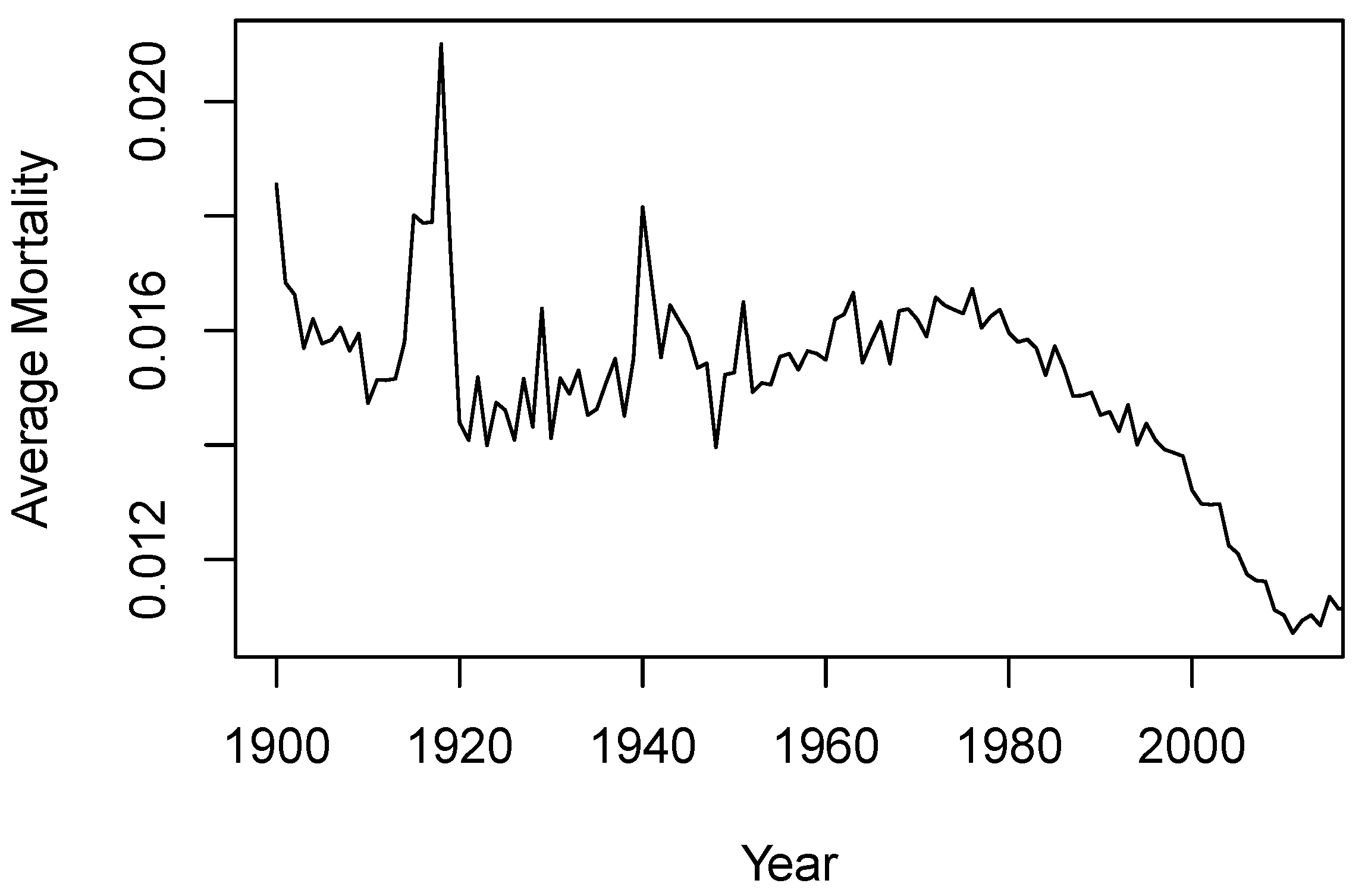
Figure 1 illustrates the average mortality rates across ages 20–95 for each year in the sample period. The average mortality rates exhibit an overall downward trend over the years. Before 1950, mortality rates were considerably volatile, while in recent years, they have become less erratic. In addition, mortality rates have been decreasing in a concave manner over the last few decades, suggesting an accelerating improvement in mortality. However, mortality stopped improving or even deteriorated slightly between 2015 and 2019, likely due to escalating drug-related deaths.

We fit the Lee–Carter model to the EW mortality data in the period of 1900–2011 and demonstrate the estimated parameters in Figure 2. $a_x$ represents the average age-specific mortality, reflecting the overall age pattern of human mortality. The decreasing $b_x$ suggests a milder response to the time-varying mortality index $k_t$ and thus diminishing mortality improvement at higher ages. The decreasing trend in the mortality index $k_t$ indicates mortality improvement over time. Additionally, $k_t$ appears to decrease faster post-1950 compared to pre-1950. The first difference in the mortality index, represented by $\Delta k_t=k_t-k_{t-1}$, was very volatile before 1950 and became relatively stable after 1950.

In Lee and Carter (1992), the mortality index $k_t$ is further modeled as a random walk with a drift. Antolin (2010) considered linear AR(1) for the first difference in the mortality index, $\Delta k_t$. This is equivalent to modeling $k_t$ with ARIMA(1,1,0). However, the plots of $k_t$ and $\Delta k_t$ suggest nonlinearity in the mean and the variance in the time series. Therefore, an ARIMA model may not be sufficient to capture the nonlinearity in the mortality index.

3. Linear and Nonlinear Time-Series Models for $\Delta k_t$

3.1. Autoregressive (AR) Model

Since AR models are widely used for $\Delta k_t$ in the existing literature, we use AR models as the baseline. We first select the number of AR lags based on the Bayesian information criterion (BIC). By penalizing extra parameters, the BIC addresses the potential overfitting problem in complex models. The formula for the BIC is

$$\mathrm{BIC}=-2ln\widehat{L}+kln\left(n\right),$$

where $\widehat{L}$ is the maximized value of the likelihood function, k is the number of parameters to be estimated, and n is the number of observations.

Table 1. BIC for AR models with different lag orders. The lowest BIC value is highlighted in bold.

AR Lag Number	0	1	2	3
BIC	671.5251	666.9721	667.3039	670.8484

summarizes the BIC values for models with different AR lag orders. We note that AR(0) is equivalent to modeling $k_t$ as a random walk with drift. It is evident that the AR(1) model yields the lowest BIC. Therefore, we use AR(1) for $\Delta k_t$.

Employing the maximum-likelihood method, the estimated AR(1) model for $\Delta k_t$ is shown as follows:

$$\Delta k_t=-1.3602-0.2830\Delta k_{t-1}+{ϵ}_t,{ϵ}_t\sim N(0,20.86)$$

(2)

The long-term mean of $\Delta k_t$ is $-1.0602$, indicating that the mortality index $k_t$ decreases at the rate of 1.0602 per year. The negative coefficient $-0.2830$ means that $\Delta k_t$ has a negative correlation with its immediate previous value $\Delta k_{t-1}$, suggesting that after an above-average mortality improvement, the following year is likely to experience a below-average mortality improvement or even a mortality deterioration, and vice versa.

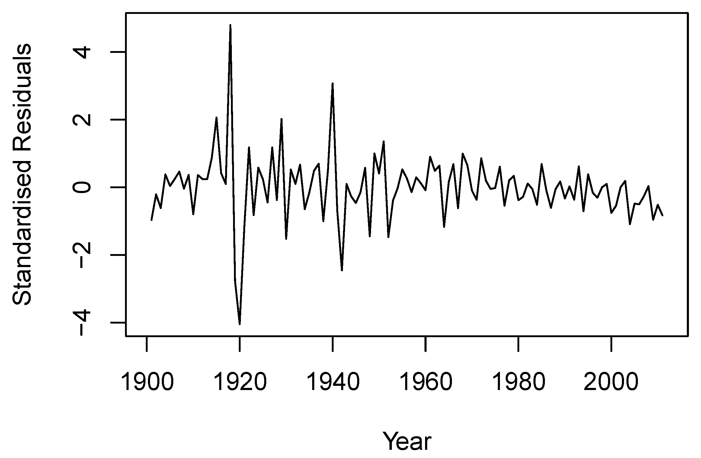
In Figure 3, we depict the standardized residuals derived from the estimated linear AR(1) model for $\Delta k_t$. While the estimated model suggests a constant variance of 20.86 for the error term, the residuals in Figure 3 reveal different volatility pre- and post-1950. The residuals also appear to have a slightly lower mean, which indicates a faster mortality improvement, in recent years. These observations suggest the presence of nonlinearity and heteroskedasticity in the residuals. To capture these features of the data, we consider four nonlinear time-series models: the TAR model, MS model, SC model, and AR-GARCH model for $\Delta k_t$ in the remainder of this section.

3.2. Threshold Autoregressive (TAR) Model

The threshold autoregressive (TAR) model was initially introduced by Tong (1978) to describe nonlinear movements in stock prices within financial markets. Comprehensive discussion and extensions of the TAR model were made by Tong and Lim (1980) and Tong (1983). The TAR model employs piece-wise AR models to accommodate deviations from linearity. In this approach, AR models are estimated separately within each time-series segment or regime defined by threshold variables. A TAR model incorporating m threshold variables for $\Delta k_t$ can be expressed as follows:

$$\Delta k_t=\left\{\begin{array}{cc}\hfill {\alpha }^{\left(1\right)}+{\beta }^{\left(1\right)}\Delta k_{t-1}+& {ϵ}_t^{\left(1\right)},\mathrm{if}\Delta k_{t-1}\le r_1\hfill \\ \\ \hfill {\alpha }^{\left(2\right)}+{\beta }^{\left(2\right)}\Delta k_{t-1}+& {ϵ}_t^{\left(2\right)},\mathrm{if}{r}_1<\Delta k_{t-1}\le r_2\hfill \\ \hfill & ⋮\hfill \\ \hfill {\alpha }^{\left(m\right)}+{\beta }^{\left(m\right)}\Delta k_{t-1}+& {ϵ}_t^{\left(m\right)},\mathrm{if}{r}_{m-1}<\Delta k_{t-1}\le r_m\hfill \\ \hfill {\alpha }^{(m+1)}+{\beta }^{(m+1)}\Delta k_{t-1}+& {ϵ}_t^{(m+1)},\mathrm{if}\Delta k_{t-1}>r_m\hfill \end{array}\right.,$$

(3)

where $r_i$ is the ith threshold value with $r_1<r_2<\cdots <r_m$, ${\alpha }^{\left(i\right)}$ and ${\beta }^{\left(i\right)}$ are the intercept and AR coefficient for the AR(1) model in regime i, and ${ϵ}_t^{\left(i\right)}$ is the error term for regime i, following a normal distribution with mean 0 and variance ${\left({\sigma }_t^{\left(i\right)}\right)}^2$. The threshold values classify the observations into $m+1$ regimes. $\Delta k_t$ switches between regimes based on the value of $\Delta k_{t-1}$. The TAR model allows the AR structure to change based on the threshold variables, thereby capturing complex nonlinearity dynamics.

To fit the TAR model, we use a two-step procedure. In the first step, we use the MLE method to estimate the TAR models with various numbers of threshold values. The threshold values are estimated together with the AR parameters using MLE. A minimum percentage of observations in each regime is set to 10%. In the second step, we compute the BIC for each estimated model and select the number of threshold values and its corresponding model to minimize the BIC.

Table 2. BIC values for TAR models with various number of regimes. The lowest BIC value is highlighted in bold.

Model	AR	TAR—2 Regimes	TAR—3 Regimes
BIC	664.3891	651.2574	657.8741

summarizes the BIC values for the AR(1) model and TAR models with two and three regimes. It is evident that the TAR model with two regimes yields the lowest BIC, indicating that the TAR model with one threshold value strikes a good balance between goodness of fit and model parsimony.

To further verify our choice of the number of threshold values, we conduct the test for threshold effects following Hansen (1999) using the bootstrap procedure. This test can be conducted in R with the tsDyn package (Stigler 2019; Di Narzo et al. 2009). The test statistics and p-values are presented in

Table 3. Tests of threshold effects.

Null	Alternative	Test Statistic	p-Value
One regime	Two regimes	29.4653	0.001
One regime	Three regimes	44.4485	0.002
Two regimes	Three regimes	11.8176	0.146

. We note that one regime represents the original AR model with no threshold, hence linearity. The very low p-values of the tests for one regime versus two regimes and one regime versus three regimes indicate that linearity is rejected at the 5% significance level for both tests. The p-value of the test for two regimes versus three regimes is 0.146, suggesting that we cannot reject two regimes in favor of three regimes at the 5% significance level. Therefore, the three tests indicate that the model with two regimes, corresponding to one threshold, is the most suitable. This aligns with our model selection based on the BIC values.

The estimated TAR model with one threshold is expressed as follows:

$$\Delta k_t=\left\{\begin{array}{c}\hfill 5.6870+0.7478\Delta k_{t-1}+{ϵ}_t^{\left(1\right)},\Delta k_{t-1}\le -4.4393\\ \hfill -1.5078-0.6543\Delta k_{t-1}+{ϵ}_t^{\left(2\right)},\Delta k_{t-1}>-4.4393\end{array}\right.,$$

(4)

where ${ϵ}_t^{\left(1\right)}\sim N(0,17.6592)$ and ${ϵ}_t^{\left(2\right)}\sim N(0,15.8532)$. The threshold $-4.4393$ divides $\Delta k_t$ into two regimes, with 18.92% of the observations in the first regime, and 81.08% in the second regime.

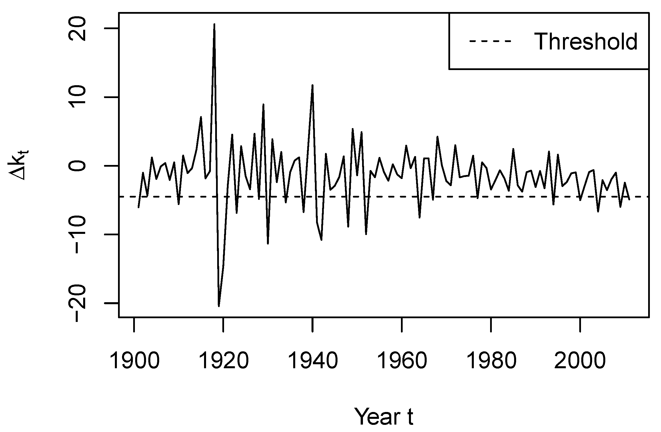
Figure 4 displays the values of $\Delta k_t$, with the estimated TAR threshold represented by the horizontal dashed line. We observe that $\Delta k_t$ enters the first regime when $\Delta k_{t-1}$ is very low, thus indicating a strong mortality improvement. Such substantial improvements likely happen in the recovery periods following catastrophe events such as pandemics or wars, which cause large mortality shocks. Therefore, the first regime occurs more often pre-1950. In addition, due to the rareness of these shocks, the first regime contains many fewer observations than the second regime.

The estimated TAR model with two regimes can be interpreted as follows. When $\Delta k_{t-1}\le -4.4393$, a higher-than-normal mortality improvement occurred at time $t-1$. Such a large negative $\Delta k_{t-1}$ usually occurs when the population recovers from a mortality shock in previous years. Based on the estimated TAR model, $\Delta k_t$ is in the first regime. The extent of mortality improvement or deterioration in year t depends on the value of $\Delta k_{t-1}$. If $\Delta k_{t-1}\le -7.6088$, we have $E(\Delta k_t\mid \Delta k_{t-1})<0$, indicating further mortality improvement in year t. This can occur when the recovery from a large mortality shock lasts multiple years. If $-7.6088<\Delta k_{t-1}\le -4.4393$, we have $0<E(\Delta k_t\mid \Delta k_{t-1})<2.3702$, indicating a mild mortality deterioration in year t. For the second regime, the threshold constraint $\Delta k_{t-1}>-4.4393$ indicates that a mild mortality improvement or a mortality deterioration occurred in year $t-1$. If $-4.4393<\Delta k_{t-1}<-2.3045$, we obtain $E(\Delta k_t\mid \Delta k_{t-1})>0$, which suggests a mortality deterioration in year t. If $\Delta k_{t-1}>-2.3045$, a mortality improvement is expected in year t.

3.3. Markov Switching (MS) Model

The Markov switching (MS) model, introduced by Hamilton (1989), is designed to capture regime shifts in time-series data where different states or regimes have distinct statistical properties. Switching between these regimes is governed by a state variable that follows a first-order Markov chain. Milidonis et al. (2011) noted that the MS model is capable of identifying the time when a shock arrives at the underlying mortality variable, thereby reflecting different natures of mortality evolution and capturing both temporary mortality shocks and permanent mortality improvements.

Similar to the TAR model, we assume that each regime is described with its own AR model. An n-state MS model can be expressed as follows:

$$\Delta k_t=\left\{\begin{array}{cc}\hfill {\stackrel{}{\alpha }}^{\left(1\right)}+{\beta }^{\left(1\right)}\Delta k_{t-1}+& {ϵ}_t^{\left(1\right)},S_t=1\hfill \\ \hfill {\alpha }^{\left(2\right)}+{\beta }^{\left(2\right)}\Delta k_{t-1}+& {ϵ}_t^{\left(2\right)},S_t=2\hfill \\ \hfill & ⋮\hfill \\ \hfill {\alpha }^{\left(n\right)}+{\beta }^{\left(n\right)}\Delta k_{t-1}+& {ϵ}_t^{\left(n\right)},S_t=n\hfill \end{array}\right.,$$

(5)

where $S_t$ is the state variable indicating the state level at time t. The error term ${ϵ}_t^{\left(i\right)}$ follows a normal distribution with mean 0 and variance ${\left({\sigma }^{\left(i\right)}\right)}^2$. When $S_t$ changes to a different value, $\Delta k_t$ switches from one AR model to another.

$S_t$ is assumed to follow a time-homogeneous first-order Markov chain. Let $p^{ij}=Pr(S_t=j\mid S_{t-1}=i)$ denote the transition probability from state i at time $t-1$ to state j at time t. The Markovian probability transition matrix P that describes the random switching between different regimes can be written as

$$\Pi =\left[\begin{array}{cccc}{p}^{11}& p^{12}& \cdots & p^{1n}\\ p^{21}& p^{22}& \cdots & p^{2n}\\ ⋮& ⋮& ⋮& ⋮\\ p^{n1}& p^{2n}& \cdots & p^{nn}\end{array}\right].$$

Let $\Theta$ represent the set of parameters in the MS model, and ${\Omega }_t$ denote the vector of $(\Delta k_{t_1},\Delta k_{t_1-1},\cdots ,\Delta k_{t_0+1})$, where $t_0$ and $t_1$ are the first and last years in the sample period, respectively. The log-likelihood function of the MS model, based on observations of $\Delta k_t$, can be expressed as follows:

$$\begin{array}{cc}\hfill & ln\left[L(\Theta \mid \Delta k_{t_1},\Delta k_{t_1-1},\cdots ,\Delta k_{t_0+1})\right]=lnf(\Delta k_{t_0+1}\mid \Theta )+\sum _{t=t_0+2}^{t_1}lnf(\Delta k_t\mid {\Omega }_{t-1},\Theta ),\hfill \end{array}$$

where f is the probability density function. We maximize the log-likelihood to obtain parameter estimates. For the detailed estimation procedure, we refer the readers to Milidonis et al. (2011).

To determine the number of regimes, we estimate the MS model with both two and three regimes and select the model with a lower BIC.

Table 4. BIC values for the MS models with various numbers of regimes. The lowest BIC value is highlighted in bold.

Model	AR	MS—2 Regimes	MS—3 Regimes
BIC	664.3891	630.4966	647.5568

presents the BIC values for the AR(1) model and two MS models. The MS model with two regimes exhibits the lowest BIC and as a result we select it for our data. The estimated model is expressed as follows:

$$\Delta k_t=\left\{\begin{array}{c}\hfill \stackrel{}{6}.1780+0.9444\Delta k_{t-1}+{ϵ}_t^{\left(1\right)},S_t=1\\ \hfill -2.2877-0.5942\Delta k_{t-1}+{ϵ}_t^{\left(2\right)},S_t=2\end{array}\right.,$$

(6)

where ${ϵ}_t^{\left(1\right)}\sim N(0,46.8930)$ and ${ϵ}_t^{\left(2\right)}\sim N(0,7.2374)$. The estimated transition matrix is

$$\Pi =\left[\begin{array}{cc}0.1733& 0.8267\\ 0.0918& 0.9082\end{array}\right].$$

The two regimes have notably different parameter estimates. The variance for the AR model in the first regime is significantly higher than that in the second regime. Therefore, the first regime represents the more volatile period for mortality improvement, while the second regime represents the more stable period.

The transition probability of $p^{12}=0.8267$ suggests that there is a very high probability of the state transiting from the volatile regime to the stable regime. However, when the state is in the stable regime, the transition probability of $p^{21}=0.0918$ suggests that it is unlikely to transit to the volatile regime. Therefore, we expect that the state variable is equal to 2 most of the time.

The AR model for the first regime has an intercept of 6.1780 and an AR coefficient of 0.9444. When a mortality deterioration occurs at time $t-1$, a significant deterioration is also expected at time t if the state at time t is 1. However, the probability of remaining in the first regime or switching to the first regime is low, 0.1733 and 0.0918, respectively. Therefore, following a mortality deterioration at time $t-1$, it is more likely that the state at time t is 2. Due to the negative intercept and coefficient in the second regime, a mortality improvement is expected at time t given state 2 at time t.

The long-term mean of $\Delta k_t$ in the second regime can be calculated as $-2.2877/(1+0.5942)=-1.434949$. Since the state variable stays in regime 2 most of the time, we expect $\Delta k_t$ to fluctuate around $-1.434949$ over the long run and, thus, $k_t$ to continue to decrease in the future.

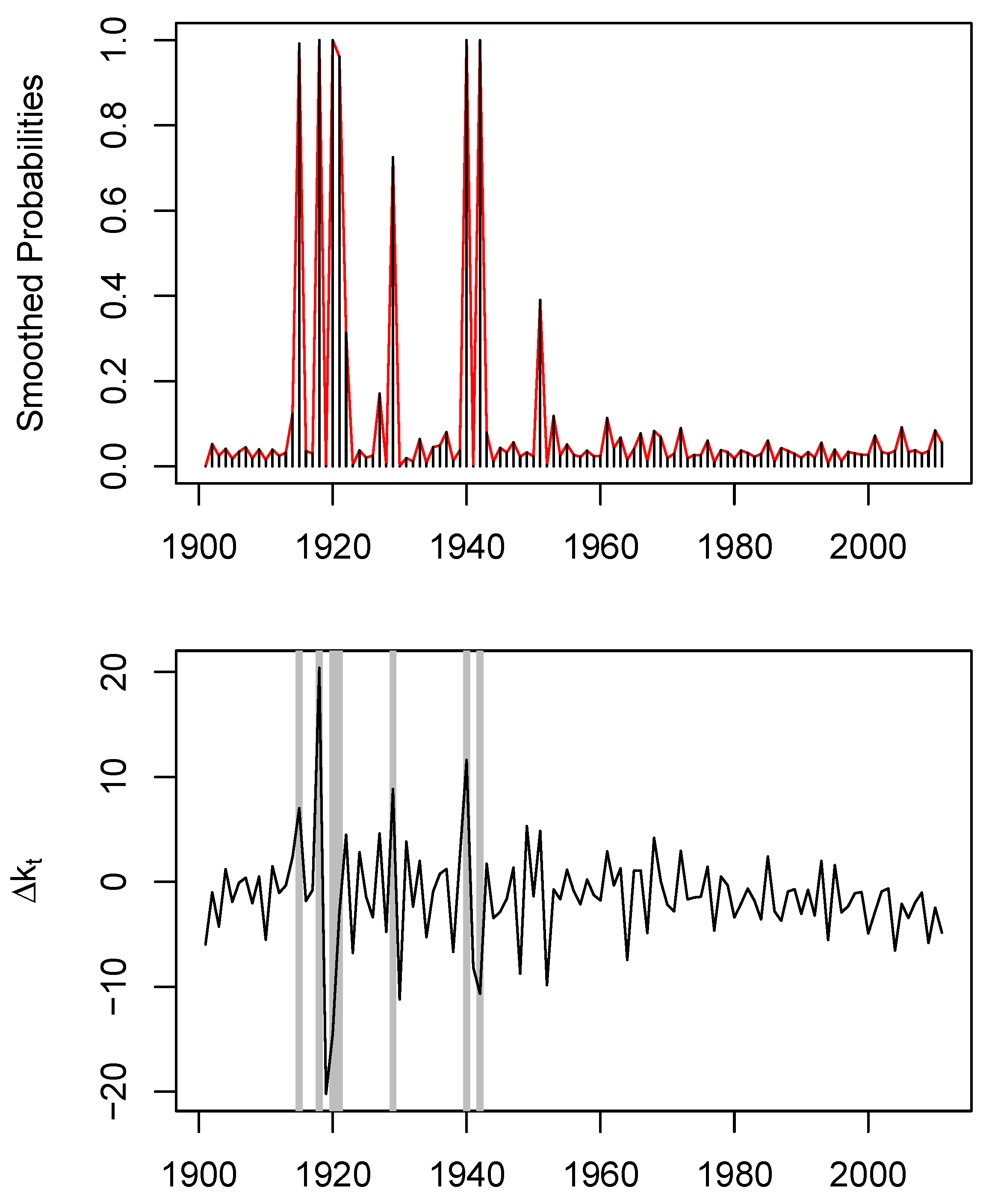
In Figure 5, we provide a plot of the smoothed probability (top panel) of $\Delta k_t$ being in the first regime given ${\Omega }_t$ alongside the values of $\Delta k_t$, with the periods of the first regime shaded in gray (bottom panel). We deem the state to be equal to 1 when the smoothed probability of being in the first regime is greater than that in the second regime. The two panels demonstrate that, given its observed value, $\Delta k_t$ exhibits a higher probability of being in regime one when $\Delta k_t$ is extremely high or low. Regime one predominantly occurs in the periods 1915–1920 and 1940–1950. These two decades coincide with periods of wars and severe flu outbreaks, characterized by high mortality variations.

3.4. Structural Change (SC) Model

The structural change (SC) model, initially introduced by Lewis (1955), originally aimed to illustrate the structural transformation from rural agriculture to urban industry due to economic growth. Recently, researchers such as Sweeting (2011) and Van Berkum et al. (2016) have explored its application in mortality modeling. Unlike the TAR and MS models, structural change is permanent. In other words, mortality improvement, $\Delta k_t$, follows a new model after each change point and never reverts to the previous model.

In an SC model, changes may manifest in various aspects, including the mean and variance. In this paper, we examine the changes in both mean and variance and assume that $\Delta k_t$ follows a piece-wise AR(1) model. Such an SC model with n change points can be written as follows:

$$\Delta k_t=\left\{\begin{array}{cc}\hfill {\stackrel{}{\alpha }}^{\left(1\right)}+{\beta }^{\left(1\right)}\Delta k_{t-1}+& {ϵ}_t^{\left(1\right)},t\le s{c}_1\hfill \\ \hfill {\alpha }^{\left(2\right)}+{\beta }^{\left(2\right)}\Delta k_{t-1}+& {ϵ}_t^{\left(2\right)},s{c}_1<t\le s{c}_2\hfill \\ \hfill & ⋮\hfill \\ \hfill {\alpha }^{\left(n\right)}+{\beta }^{\left(n\right)}\Delta k_{t-1}+& {ϵ}_t^{\left(n\right)},s{c}_{n-1}<t\le s{c}_n\hfill \\ \hfill {\alpha }^{(n+1)}+{\beta }^{(n+1)}\Delta k_{t-1}+& {ϵ}_t^{(n+1)},t>s{c}_n\hfill \end{array}\right.,$$

(7)

where $s{c}_j$ is the time or location of the jth detected change point and the error term ${ϵ}_t^{\left(i\right)}$ follows a normal distribution with mean 0 and variance ${\left({\sigma }^{\left(i\right)}\right)}^2$. This framework allows us to capture the varying patterns of the time series due to structural changes.

The n change points divide the time series into $n+1$ regimes. Given the number and location of the change points, we can estimate the AR model for each regime using the observations in the regime with MLE. Assuming that there is only one change point, we take the following procedures to determine the location of the change point:

• For each value of $s{c}_1$ in $1912,1913,\dots ,2000$, estimate the SC model and compute the corresponding BIC value.
• Select the value for $s{c}_1$ that minimizes the BIC.

We consider the range of $[1912,2000]$ for $s{c}_1$ to ensure a minimum of 10% observations in each regime. For two change points, the ranges for $s{c}_1$ and $s{c}_2$ are $[1902,2000]$ and $[s{c}_1+11,2000-11]$, respectively. For each combination of $t_1$ and $t_2$, we estimate the corresponding SC model and compute its BIC. We select the combination of $t_1$ and $t_2$ that minimizes the BIC.

Similar procedures are taken for three or more change points. The optimal number of change points is selected to minimize the BIC of the resulting SC model. In

Table 5. BIC values for the SC models with various numbers of change points. The lowest BIC value is highlighted in bold.

	AR(1)	One Change Point	Two Change Points	Three Change Points
BIC	664.3891	633.6326	633.8307	643.0997

, we provide the BIC values for the SC models with various numbers of change points. The model with one change point yields the lowest BIC. The optimal change point location for this model is 1952.

The selected SC model is expressed as follows:

$$\Delta k_t=\left\{\begin{array}{cc}\hfill \stackrel{}{-}1.1528-0.2869\Delta k_{t-1}+{ϵ}_t^{\left(1\right)},& t\le 1952\hfill \\ \hfill -1.5149-0.3053\Delta k_{t-1}+{ϵ}_t^{\left(2\right)},& t>1952\hfill \end{array}\right.,$$

(8)

where ${ϵ}_t^{\left(1\right)}\sim N(0,37.7)$ and ${ϵ}_t^{\left(2\right)}\sim N(0,5.153)$.

In the fitted structural change model, the observations of $\Delta k_t$ are divided into two segments. The first regime comprises 46.85% of the observations, while the second regime accounts for 53.15% of the observations. It is interesting to note that the estimates of the intercept and AR coefficient for the two regimes are not as drastically different as we have seen in the TAR and MS models. However, the estimates of the variance are significantly different in the two regimes. Prior to 1952, $\Delta k_t$ was in the first regime, marked by significant volatility due to major mortality jumps in 1920 and 1940. From 1952 onward, $\Delta k_t$ is in the second regime with relative stability, as the Second World War had ended and no events that had a significant impact on mortality occurred in this period.

The long-term means for the two regimes are $-0.8958$ and $-1.1606$, respectively, indicating that mortality improvement occurs in both segments, with higher improvement in regime two. Mortality improvement accelerates in the second regime due to medical advances and the strengthened health system. This aligns with our observations of accelerating mortality improvement in recent decades in Figure 1.

3.5. AR-GARCH Model

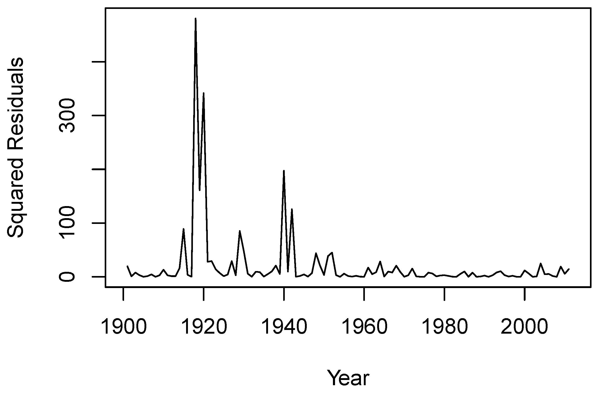
To determine if an AR-GARCH model is an appropriate choice for our dataset, we first examine the squared residuals from the fitted AR(1) model, as illustrated in Figure 6. We observe periods of spikes in volatility around the years 1918, 1929, 1940, and 1950, which suggest the potential existence of volatility clustering.

Further analysis is presented in the autocorrelation function (ACF) and partial autocorrelation function (PACF) plots for the squared residuals, as shown in Figure 7. The significant values at the first and second lags in both ACF and PACF imply that there is a correlation in volatility over different lags. This supports the presence of volatility clustering and, thus, the use of a GARCH model for our data.

A GARCH$(q,p)$ model for the conditional variance is expressed as follows:

$$\begin{array}{ccc}\hfill {ϵ}_t& =& z_t{\sigma }_t,\hfill \\ \hfill {\sigma }_t^2& =& \omega +\sum _{i=1}^q{\alpha }_i{ϵ}_{t-i}^2+\sum _{j=1}^p{\beta }_j{\sigma }_{t-j}^2,\hfill \end{array}$$

where ${ϵ}_t$ is the error term from the AR model, ${\sigma }_t$ is the time-varying volatility, $z_t$ follows a standard normal distribution, p is the order of the GARCH terms, and q is the order of the ARCH terms. To ensure that the model is statistically valid and that the volatility predictions are non-negative and stationary, the following parameter constraints are imposed: $\omega >0$, ${\alpha }_i>0$ for $i=1,\dots ,q$, ${\beta }_i>0$ for $j=1,\dots ,p$, and ${\sum }_{i=1}^q{\alpha }_i+{\sum }_{j=1}^p{\beta }_j<1$. We estimate the AR-GARCH model in one step by maximizing its log-likelihood using the rugarch package (Galanos 2023).

To determine the orders for the GARCH model, we use the BIC as the selection metric. Observations from the ACF and PACF plots of the squared residuals, which exhibit significant values at lags 1 and 2, suggest that the values of p and q do not exceed 2. The BIC values for various GARCH model specifications, with $p\le 2$ and $q\le 2$, are presented in

Table 6. BIC values for the AR-GARCH model with various values for the ARCH order q and GARCH order p. The lowest BIC value is highlighted in bold.

$(\mathit{q},\mathit{p})$	(0,0)	(1,0)	(1,1)	(1,2)	(2,1)	(2,2)
BIC	664.3891	654.1983	639.1149	641.6136	636.7701	641.4797

. Note that the GARCH(0,0) variance is equivalent to an AR(1) model. The GARCH(2,1) model emerges as the best choice, indicated by the lowest BIC value among the considered models.

The selected AR-GARCH model is written as follows:

$$\begin{array}{ccc}\hfill \Delta k_t& =& -1.4521-0.4960\Delta k_{t-1}+{ϵ}_t,\hfill \\ \hfill {\sigma }_t^2& =& 3.0991+0.12929{ϵ}_{t-1}^2+0.5540{ϵ}_{t-2}^2+0.3157{\sigma }_{t-1}^2.\hfill \end{array}$$

The positive ARCH and GARCH coefficients imply that a large shock in the previous two periods or high conditional variance in the previous period has a positive impact on the conditional variance in the current period.

3.6. Model Comparison

Table 7. BIC values for various linear and nonlinear models. The lowest BIC value is highlighted in bold.

	One Regime	Two Regimes	Three Regimes
AR	664.3891
TAR		651.2574	657.8741
MS		630.4966	647.5568
SC		633.6326	633.8307
AR-GARCH	636.7701

compiles the BIC values obtained by fitting different time-series models to the EW mortality data. We observe that all four nonlinear models exhibit lower BIC values compared to the linear AR(1) model. This observation suggests that nonlinear models provide a significantly better fit than the AR(1) model and highlights the importance of properly modeling the nonlinear trend in mortality improvement.

Among all the models we fitted, the MS model with two regimes stands out as the best fit. MS models offer a transparent representation of structural changes in mortality. As pointed out by Milidonis et al. (2011), these models provide flexibility in choosing the switching time, duration, and parameter estimates through maximum-likelihood estimation. These properties collectively contribute to the excellent fit of the MS model to the mortality data.

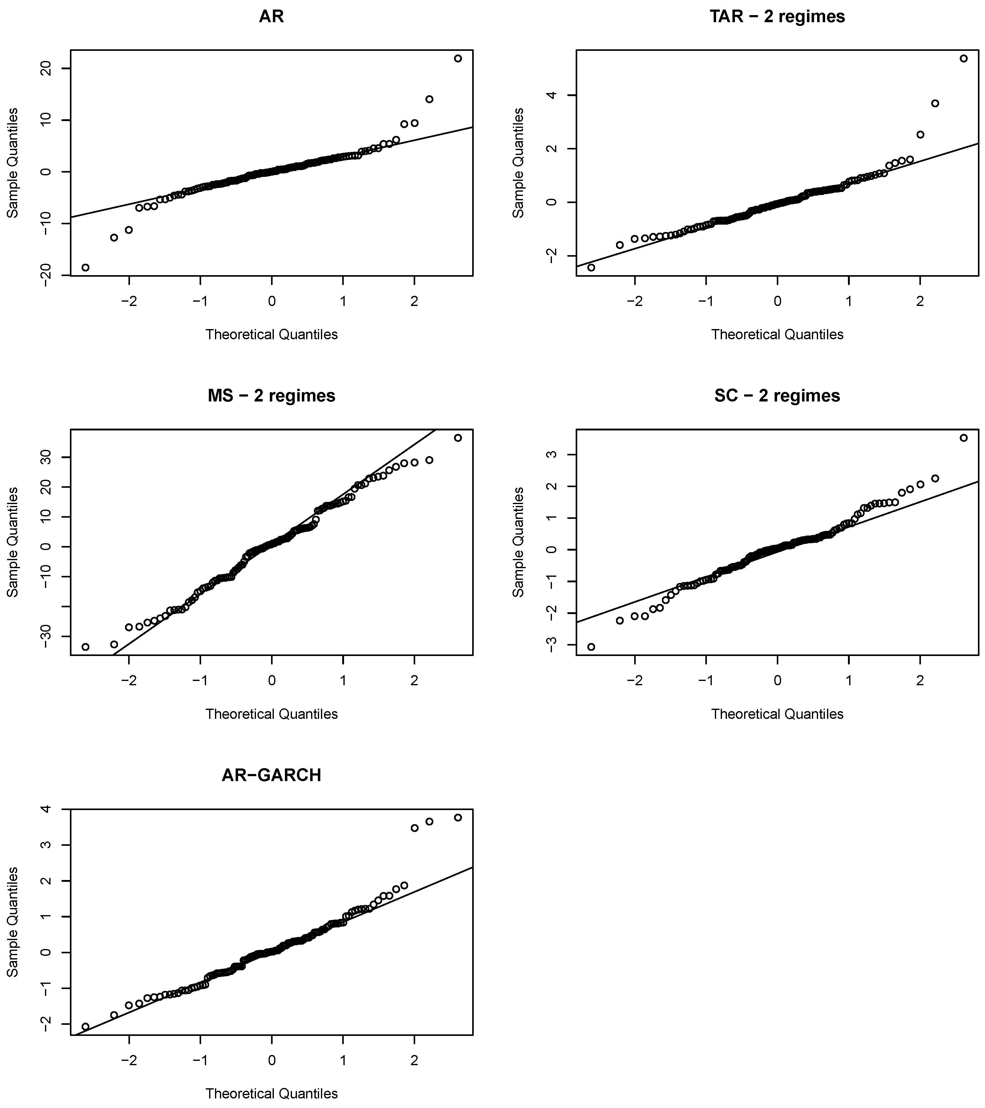
In Figure 8, we present QQ plots of residuals to assess the normality assumptions for both linear and nonlinear models. The QQ plot for the AR(1) model deviates from the expected normality line, exhibiting heavier tails on both the left and right. In contrast, the QQ plots for the nonlinear models generally follow a more linear pattern, suggesting that their residuals are closer to normality than the residuals from the AR(1) model. While both TAR and AR-GARCH alleviate the heavy left tail, especially for extremely low values of $\Delta k_t$, they still display a pronounced heavy right tail. Both the MS and SC models, however, seem to effectively mitigate the heavy tails on both ends.

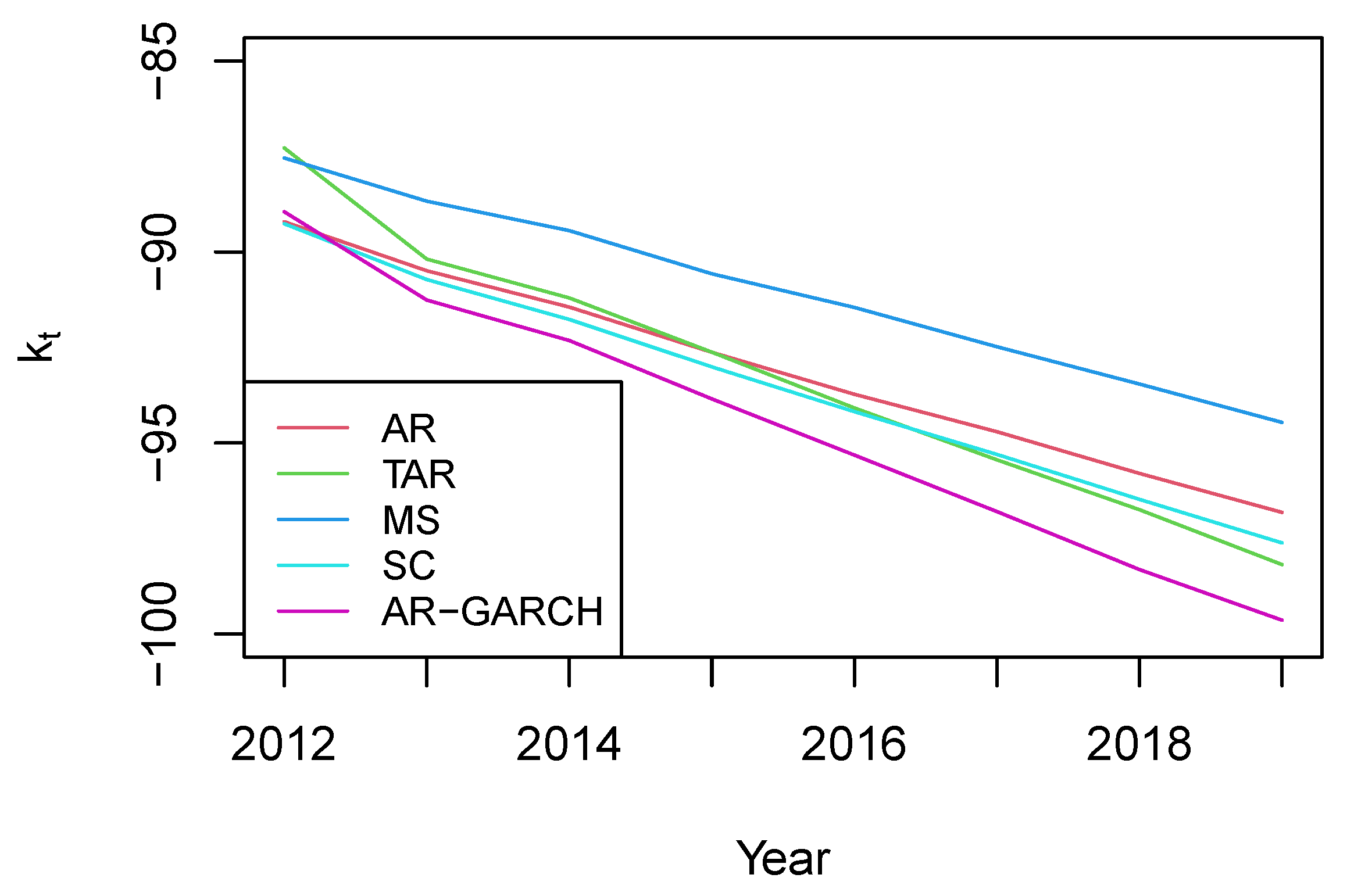
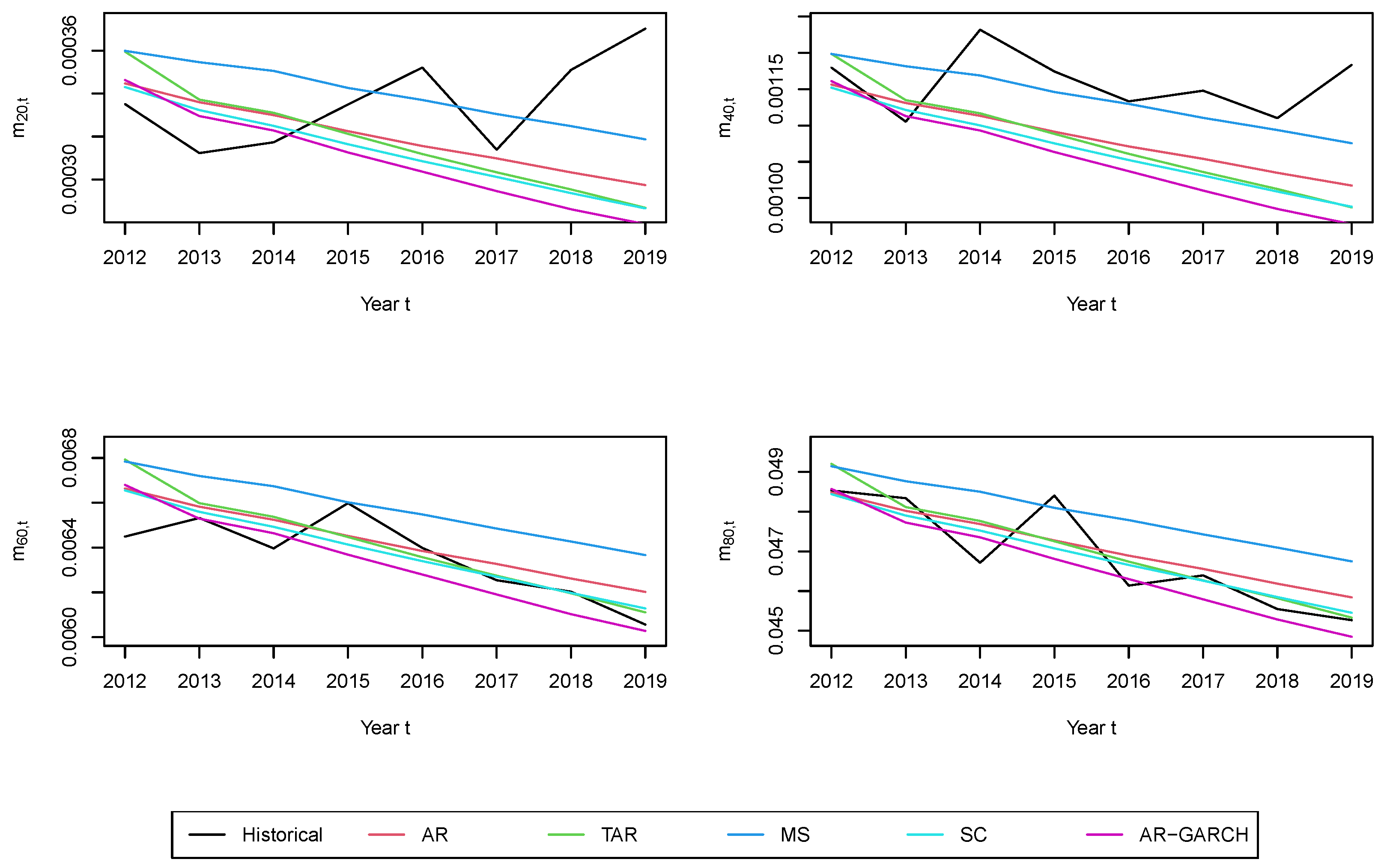
We further assess the performance of the five different models for an 8-year out-of-sample mortality forecast. We first simulate 5000 paths for the mortality index $k_t$, for $t=2012,\dots ,2019$. The simulation procedures for $k_t$ are presented in Appendix A. Figure 9 presents the mean forecasts of $k_t$ from different models. The forecasts from the AR, TAR, and SC closely align, while the mean forecasts from the MS model are significantly higher. This discrepancy may be attributed to the inclusion of a small probability of transitioning into the first regime which has a large intercept and high volatility in the MS model. In addition, the AR-GARCH model yields the lowest mean forecasts.

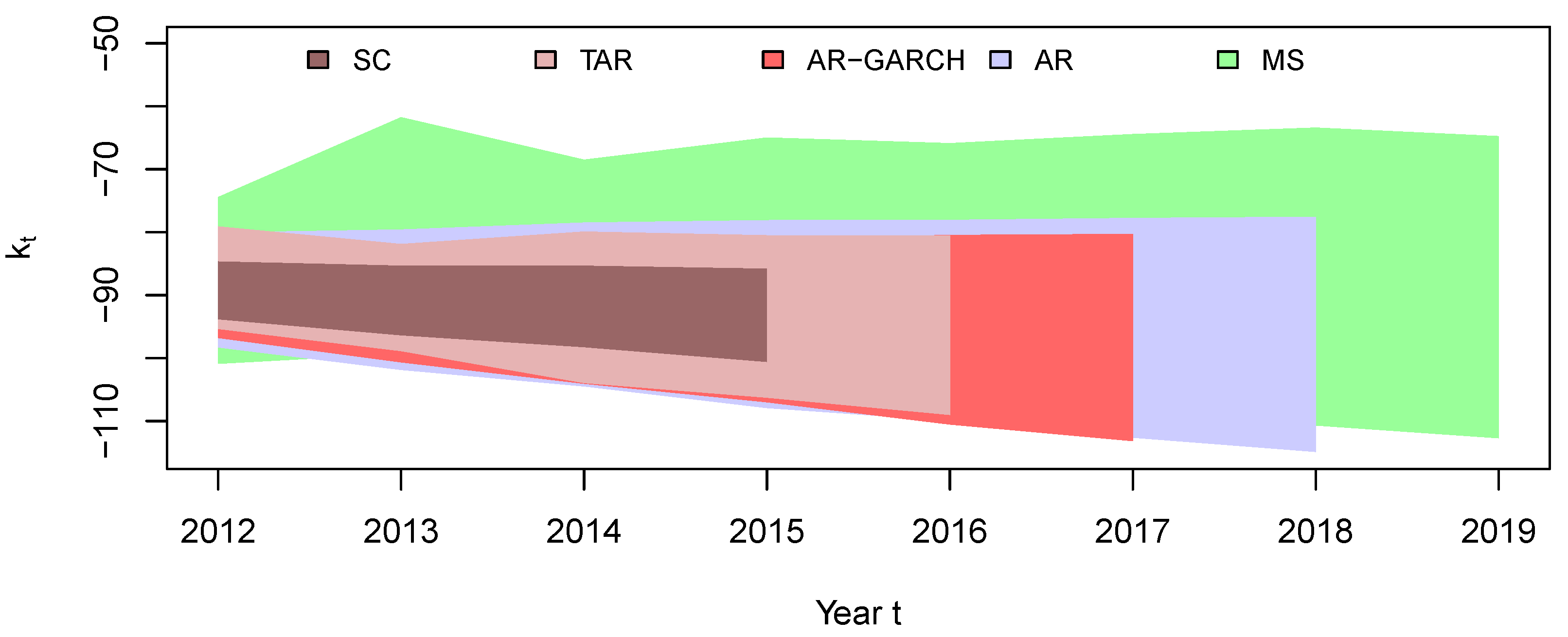
Figure 10 presents the 95% prediction interval of $k_t$ using the four models. It is very interesting to see that the MS model results in the widest prediction interval, while the SC model yields the narrowest interval. This discrepancy can be explained by the SC model’s assumption that the process remains in the second regime post-1952 and follows the fitted AR(1) model from the second regime for future mortality predictions. Since the second regime primarily consists of periods with relatively low volatility, the simulated $k_t$ experiences reduced volatility.

The simulated paths for future mortality rates are determined using the simulated paths for $k_t$ and the estimated values for $a_x$ and $b_x$. Figure 11 illustrates the mortality forecasts at four ages—20, 40, 60, and 80—and compares them with the observed rates. The MS model performs relatively better for ages 20 and 40, but worse for ages 60 and 80. The predicted mortality rates from the AR, TAR, and SC models are close to each other, while the predicted rates from the AR-GARCH model are consistently the lowest.

Furthermore, we quantify the mean squared error for a forecast period of i across ages 20–95 as follows:

$$MS{E}_i=\sum _{x=20}^{95}\frac{1}{76}{({\widehat{m}}_{x,2011+i}-m_{x,2011+i})}^2,$$

where ${\widehat{m}}_{x,2011+i}$ is the predicted mortality rate for an individual aged x in year $2011+i$. Figure 12 plots the mean squared errors for $i=1,\dots ,8$. The MS model outperforms the other three models for most of the forecast periods.

Finally, we average the mean squared errors across all forecast periods (1–8 years) as follows:

$$MSE=\frac{{\sum }_{i=1}^{8}MS{E}_i}{8}.$$

The MSEs using different models are presented in

Table 8. Overall mean squared errors for mortality predictions using the five models. The lowest MSE value is highlighted in bold.

Model	AR	TAR	MS	SC	AR-GARCH
MSE ($\times {10}^{-5}$)	1.7149	1.7407	1.4176	1.8030	1.9757

. The MS model again yields the lowest overall mean squared error. Surprisingly, the AR(1) model, which does not consider any nonlinearity, performs the second best. The AR-GARCH model performs the worst among all five models and the SC model is the second worst. The existing literature often uses the SC approach implicitly by choosing a more recent starting year for the dataset and avoiding the periods with jumps and outliers. However, our out-of-sample results suggest that removing the observations in the early years may not necessarily lead to a good prediction for future mortality rates.

4. Analysis with Different Base Mortality Structures and Population Data

4.1. Age–Period–Cohort Model

The choice of a base mortality structure is important, as it can significantly influence the mortality forecasts and, consequently, impact the outcomes of model comparisons. In addition to the Lee–Carter model, our study also incorporates the age–period–cohort (APC) model to provide a broader perspective. The APC model (Holford 1983) is formulated as

$$ln\left(m_{x,t}\right)=a_x+k_t+g_{t-x},$$

where $a_x$ denotes the age effect, $k_t$ represents the period effect, paralleling their interpretations within the Lee–Carter framework, and $g_{t-x}$ is the cohort effect specific to each birth year. To ensure the identifiability of the APC model parameters, the following constraints are imposed:

$$\sum _t{k}_t=0,\sum _c{g}_c=0,\sum _{c}c{g}_c=0.$$

The APC model is estimated with the maximum-likelihood method using the StMoMo package (Villegas et al. 2018) in this paper.

In

Table 9. BIC values for five different models of $k_t$ and the corresponding MSEs of predicted mortality rates, using the APC structure and EW mortality data. The lowest BIC and MSE values are highlighted in bold.

	BIC	MSE ($\times {10}^{-5}$)
AR	$-337.9807$	6.9663
TAR	−353.9411	7.3526
MS	−367.0603	6.4387
SC	−385.1734	4.6970
AR-GARCH	−376.2497	7.0572

, we present the BIC values for five different models of $k_t$ and the corresponding MSEs based on the APC structure. The calculation of the MSE here is restricted to mortality rates for individuals aged 28 to 95 in 2012–2019, to avoid the prediction of cohort effects. Interestingly, the SC model, when applied within the APC framework, exhibits the lowest BIC and MSE. Conversely, the TAR model shows the second-highest BIC and the highest MSE.

4.2. Italian Mortality Data

To evaluate the robustness of the findings derived from the EW data, we extend our analysis to the Italian mortality data. Using the same sample period and age range as used for the EW data, we obtain the BIC values for the $k_t$ models, as well as the MSEs for the Italian mortality forecasts. Both the Lee–Carter and the APC structures are considered to provide a comprehensive comparison. We present the results in

Table 10. BIC values for five different models of $k_t$ and the corresponding MSEs for predicted mortality rates, using the Italian mortality data. The lowest BIC and MSE values are highlighted in bold.

	Lee–Carter		APC
	BIC	MSE ($\times {\mathbf{10}}^{-\mathbf{6}}$)	BIC	MSE ($\times {\mathbf{10}}^{-\mathbf{5}}$)
		(Ages 20–95)		(Ages 28–95)
AR	751.0609	5.9628	−214.6237	4.6322
TAR—two regimes	746.9563	5.5745	−246.1965	5.0188
MS—two regimes	685.5103	5.7972	$-278.2540$	5.5853
SC—two regimes	700.4562	5.4884	−289.2773	2.8150
AR-GARCH	716.4090	6.0126	−305.0569	4.2920

.

Irrespective of the chosen base mortality structure, the AR model consistently yields the highest BIC value, suggesting that it has the worst goodness of fit among the models considered. However, the AR model does not necessarily result in the highest MSE for the forecast future mortality rates.

Using the Lee–Carter structure, the MS model again achieves the lowest BIC, indicating a superior goodness of fit, whereas the SC model attains the lowest MSE representing the most accurate mortality rate forecasts. Despite the substantial difference in BIC values across the different models for $k_t$, the MSE values exhibit small fluctuation. When applying the APC structure, the AR-GARCH model emerges with the lowest BIC. The SC model yields the lowest MSE of 2.8150, a significant improvement from the highest MSE of 5.5853 presented by the MS model. The comparison of the Italian results with those from the EW data reveals that there is no single model with consistently superior performance for both goodness of fit and forecasting accuracy.

5. Longevity Bond Pricing

5.1. A Longevity Bond Trade

In this section, we study how the model choice for $\Delta k_t$ may affect the price of a longevity bond. Suppose we have two counterparties involved in longevity bond trading: counterparty A, with life contingent liabilities, and counterparty B, an investor interested in the longevity bond for risk premiums. For simplicity, we assume that counterparty A sponsors a pension plan that covers one pensioner aged 65 and one pensioner aged 66 at the beginning of the year 2012. This plan pays out $1 at the end of the year if a pensioner is still alive, and the payments cease when the pensioner dies or reaches age 90. The pension payment made by counterparty A at time t is denoted by $f_t$ and expressed as follows:

$$f_t=\prod _{i=0}^{t-1}(1-q_{65+i,2012+i})+\prod _{i=0}^{t-1}(1-q_{66+i,2012+i})$$

Counterparty B sells a T-year longevity bond to counterparty A to earn risk premiums. The bond payment at time t, which includes coupons and principal repayment, is $s_t$ for $t=1,\dots ,T$.

Let us assume that Q represents the quantity of longevity bonds agreed upon by both counterparties A and B at the price of P. In Figure 13, we depict the cash flow of this transaction. At the beginning of 2012, counterparty A purchases Q units of longevity bond and pays the price of P for each unit. At time t, counterparty A pays out $f_t$ to pensioners and receives the bond payment $s_t$ from counterparty B. When the mortality of the EW population improves, pensioners live longer. Consequently, counterparty A has an extended obligation to pay pension benefits. The bond payment also increases, effectively offsetting the rise in pension liability payments for counterparty A.

We can also allow counterparty A to issue a longevity bond. In such scenarios, the quantity Q will be negative. Such a bond should be designed to make decreasing payments with higher mortality improvement. In this section, we consider two bond payment structures to illustrate how the choice of nonlinear model may affect bond prices.

5.2. Economic Pricing

The economic pricing approach was first applied to mortality-linked securities by Zhou et al. (2015), who considered the pricing problem from fundamental economic concepts of supply and demand. It assumes that buyers and suppliers aim to maximize their expected terminal utility, and market equilibrium is reached when supply equals demand.

Let $W_0^A$ and $W_0^B$ be the initial wealth of counterparties A and B, and $W_T^A$ and $W_T^B$ be the wealth at the expiration of the bond. Zhou et al. (2015) assumed that the only alternative investment is to deposit in a bank that earns a continuously compounded annual risk-free interest rate of r. Given the longevity bond price P, $Q^A$ and $Q^B$ are quantities that counterparty A is willing to purchase and counterparty B has agreed to sell at the outset of the transaction. We have the following equations for the terminal wealth:

$$\begin{array}{cc}\hfill & W_T^A(P,Q^A)=W_0^A{e}^{rT}+Q^A{e}^{rT}(\sum _{t=1}^T{s}_t{e}^{-rt}-P)-\sum _{t=1}^T{f}_t{e}^{r(T-t)},\hfill \\ \hfill & W_T^B(P,Q^B)=W_0^B{e}^{rT}+Q^B{e}^{rT}(P-\sum _{t=1}^T{s}_t{e}^{-rt}).\hfill \end{array}$$

Denote $U^A$ and $U^B$ as the utility functions of counterparties A and B, respectively. Assuming an exponential utility function, the terminal utility can be expressed as

$$\begin{array}{cc}\hfill & U^A\left(W_T^A\right)=1-e^{-c^A{W}_T^A},\hfill \\ \hfill & U^B\left(W_T^B\right)=1-e^{-c^B{W}_T^B},\hfill \end{array}$$

where $c^A$ and $c^B$ are the absolute risk aversion parameters for A and B, respectively. Counterparty A purchases longevity bonds as a means to hedge its longevity risk, while counterparty B accepts the longevity risk in pursuit of earning premiums. Consequently, it is reasonable to assume that counterparty A is more risk-averse. We assume that $c^A$ and $c^B$ are 3 and 1, respectively.

Let $F_T$ represent the accumulated pension benefit payment at time T, and $S_T$ represent the accumulated bond coupon payments at time T. We then have

$$F_T=\sum _{t=1}^T{f}_t{e}^{r(T-t)}\mathrm{and}{S}_T=\sum _{t=1}^T{s}_t{e}^{r(T-t)}.$$

Given a price P, counterparties A and B maximize their expected terminal utility. The maximization problem can be written as follows:

$$\begin{array}{cc}\hfill & Q^A={\mathrm{argmax}}_{Q^A}E\left[U^A\left(W_T^A(P,Q^A)\right)\right],\hfill \\ \hfill & Q^B={\mathrm{argmax}}_{Q^B}E\left[U^B\left(W_T^B(P,Q^B)\right)\right].\hfill \end{array}$$

First, we maximize the expected terminal utility for A. Recall that $W_T^A=W_0^A{e}^{rT}+Q^A{e}^{rT}(S_T-P)-F_T$. The conditions for maximizing the expected utility function of A are

$$\frac{\partial }{\partial Q^A}E(U^A(W_T^A(P,Q^A))=0\mathrm{and}\frac{{\partial }^2}{{\partial }^2{Q}^A}E(U^A(W_T^A(P,Q^A))<0.$$

The first condition can be rewritten as

$$E\left[c^A(S_T-e^{rT}P)e^{-c^A{Q}^A(S_T-e^{rT}P)+c^A{F}_T}\right]=0,$$

which implies

$$P=\frac{E\left[e^{-c^A{Q}^A{S}_T+c^A{F}_T}{S}_T\right]}{e^{rT}E\left[e^{-c^A{Q}^A{S}_T+c^A{F}_T}\right]}.$$

Next, we maximize the expected utility for counterparty B. Recall that the terminal wealth of counterparty B is $W_T^B=W_0^B{e}^{rT}+Q^B{e}^{rT}(P-S_T)$. The conditions for maximizing the expected utility of B are

$$\frac{\partial }{\partial Q^B}E(U^B(W_T^B(P,Q^B))=0\mathrm{and}\frac{{\partial }^2}{{\partial }^2{Q}^B}E(U^B(W_T^B(P,Q^B))<0.$$

The first condition can be rewritten as

$$E\left[c^B(S_T-e^{rT}P)e^{c^B{Q}^B(S_T-e^{rT}P)}\right]=0,$$

which implies

$$P=\frac{E\left[e^{c^B{Q}^B{S}_T}{S}_T\right]}{e^{rT}E\left[e^{c^B{Q}^B{S}_T}\right]}.$$

The market equilibrium is achieved when $Q^A=Q^B$. Therefore, P and Q, the equilibrium trading price and quantity, should satisfy the following equality:

$$P=\frac{E\left[e^{-c^{A}Q{S}_T+c^A{F}_T}{S}_T\right]}{e^{r_{f}T}E\left[e^{-c^{A}Q{S}_T+c^A{F}_T}\right]}=\frac{E\left[e^{c^{B}Q{S}_T}{S}_T\right]}{e^{rT}E\left[e^{c^{B}Q{S}_T}\right]}.$$

(9)

To calculate the expectations in Equation (9), we first simulate 5000 mortality paths and determine the simulated values of the variables inside the expectation. The expectation is then obtained by taking the average of these simulated values.

5.3. Longevity Bond on Survival Probabilities

We first consider a longevity bond with payment associated with survival probabilities. The annual coupon payable at time t is the approximate survival rate of a 65-year-old cohort. There is no principal repayment. The bond payment at time t is expressed as follows:

$$s_t=\prod _{i=0}^{t-1}(1-m_{65+i,2012+i}),t=1,\dots ,8.$$

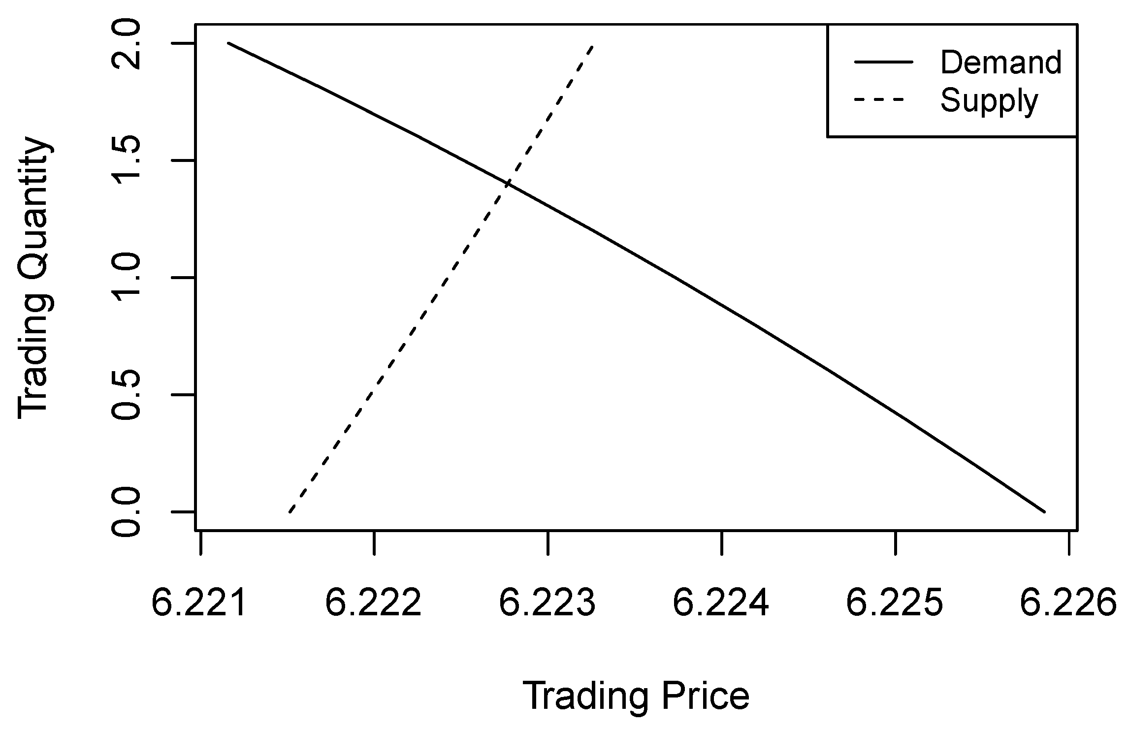
Assume that the risk-free rate r is 4.5%. Taking the MS model with two regimes as an example, we plot the supply and demand curves for this bond in Figure 14 where the intersection of the supply and demand curves represents the market equilibrium. Counterparty A, being more risk-averse, demands fewer longevity bonds as the price increases. Conversely, counterparty B, who is willing to take on more risk, is inclined to sell more bonds when the price rises.

Table 11. Pricing results for the longevity bond on survival probabilities based on mortality forecasts from various models.

	AR	TAR	MS	SC	AR-GARCH
P	6.2283	6.2275	6.2227	6.2293	6.2312
Q	1.4039	1.4121	1.4010	1.4026	1.4043
EPV	6.2277	6.2271	6.2214	6.2292	6.2309

summarizes the trading price and quantity at market equilibrium and the expected present value (EPV) of future bond payments, which is expressed as $EPV=E\left[S_T{e}^{-rT}\right]$, based on the mortality forecasts using the five models.

The trading prices obtained from the AR, TAR, and SC models are remarkably close to each other and are higher than the prices derived from the MS model. This consistency in pricing can be attributed to the very close mean forecasts of the mortality index produced by these three models, as seen in Figure 9. As we observed earlier, the mean mortality forecasts generated by the AR, TAR, and SC models are all significantly lower than those of the MS model. Consequently, this leads to a higher survival rate, increased longevity bond payments, and ultimately higher bond prices, compared to the MS model.

The price of the longevity bond obtained through the AR-GARCH model is the highest among the prices obtained from all models. The AR-GARCH model predicts a cohort survival rate that is substantially higher, leading to increased bond payments. The pension plan sponsor, facing a prolonged period of pension benefit payouts, is willing to pay a higher price to hedge against the heightened longevity risk.

Furthermore, when we examine the EPV of bond payments across different models, we observe that the MS model generates the lowest EPV, while the AR-GARCH model yields the highest EPV. This consistency in results reinforces the findings obtained through the economic pricing.

The variation in bond prices across different models is relatively minor, despite noticeable disparities in mortality rates across age groups. This observation can be attributed to the bond’s payment structure, which is based on the summation of approximate survival rates. For instance, a 5% uptick in a mortality rate $m_{x,t}$ of 0.02 translates to just around a 0.1% reduction in the corresponding approximate survival rate $(1-m_{x,t})$. Hence, employing a different bond payment structure might lead to more pronounced price differences.

5.4. Longevity Bond on Mortality Improvement Rates

We further consider a longevity bond with payments associated with mortality improvement rates. This bond is initially offered at a nominal issue price of unity, thus $P=1$. It makes an annual coupon payment of $100(e^{0.045}-1)\%+\lambda$, where $\lambda$ represents the yield spread, serving as compensation for the associated risk. The principal repayment of this bond is linked to a predefined mortality improvement index. This index, calculated as the average mortality improvement rate over the period 2012–2019 and the age range 65–89, is expressed as follows:

$$\mathrm{Index}=\frac{1}{25}\sum _{x=65}^{89}\left[1-{\left(\frac{m_{x,2019}}{m_{x,2011}}\right)}^{\frac{1}{8}}\right].$$

The principal repayment at expiration is defined as follows:

$$PR=1-max\left(min\left(\frac{\mathrm{Index}-2\%}{3\%-2\%},1\right),0\right).$$

A full principal repayment of 1 is made when the average mortality improvement remains below 2%, termed the “attachment point”. Should the index exceeds 2%, the principal repayment is reduced proportionately with the increase in the index. The principal repayment drops to zero when the index exceeds the “detachment point” of 3%. To quantify the risk of principal reduction, we define the probability of first loss as follows:

$$PFL=Pr(PR<1).$$

The bond payment at time t can be expressed as follows:

$$s_t=\left\{\begin{array}{cc}100(e^{0.045}-1)\%+\lambda & t=1,\dots ,7\\ 100(e^{0.045}-1)\%+\lambda +RP& t=8.\end{array}\right.$$

Since the issue price of the bond is already given, the pricing of this bond is equivalent to finding the spread $\lambda$.

Table 12. Pricing results for the longevity bond on mortality improvement rates based on mortality forecasts from various models.

	AR	TAR	MS	SC	AR-GARCH
$\lambda$ (basis points)	64.21	61.47	32.40	12.21	73.51
Q	$-0.0828$	$-0.0725$	$-0.1174$	$-0.1143$	$-0.0574$
Probability of first loss	10.82%	10.46%	5.62%	0.92%	11.38%

summarizes the pricing results for this bond. The negative values of Q imply that counterparty A is in the position of selling the bond. As the probability of the first loss, indicated by $PFL$, increases, the required spread $\lambda$ also increases. This is because a higher $PFL$ suggests a lower expected principal repayment, prompting investors to demand a higher risk premium to compensate for the anticipated decrease in principal.

The spread $\lambda$ shows significant variation when priced under different nonlinear models. The variation in the spread is influenced by both the average predicted mortality improvements and their volatility. The AR-GARCH model generates the highest spread, aligning with the observations from Figure 9 and Figure 10 that the AR-GARCH model leads to the fastest average mortality improvement, with moderate volatility. The considerable increase in average mortality improvement leads to a greater chance of crossing the attachment point. On the other hand, the SC model predicts the lowest spread. Even though the SC model forecasts a mean mortality improvement similar to the TAR and AR models, as shown in Figure 9, it has a very low variation in its predictions, as seen in Figure 10. Consequently, the simulations mostly yield improvement rates tightly grouped around a narrow range of values, with only 0.92% of the simulated improvement rates exceeding the attachment point of 2.5%. The MS model, which predicts the slowest mortality improvement, leads to the second-lowest spread due to its slower improvement rate outweighing the effect of its higher variance.

6. Conclusions

In this paper, we conduct a thorough analysis of various nonlinear time-series models for the mortality index in the Lee–Carter and APC structures. We assess the goodness of fit of these models and examine how the choice of the nonlinear model affects mortality forecasts and subsequently longevity bond pricing. We focus on four specific nonlinear models: TAR, MS, SC, and GARCH, using mortality data from EW and Italy from 1900 to 2019.

All four nonlinear models demonstrated lower BIC values and more normally distributed residuals than the AR model. This signifies that nonlinear models offer significant improvements in fitting mortality data. Applying the Lee–Carter structure, the MS model with two regimes emerged as the best fit for both the EW and Italian mortality data. Under the APC structure, the SC model and the AR-GARCH model achieve the lowest BIC for EW and Italian mortality, respectively.

For an eight-year out-of-sample period, we obtain the mean squared errors and prediction intervals of mortality forecasts. Applying the Lee–Carter structure, the MS and SC models lead to the lowest MSE for EW and Italian mortality, respectively. The SC model yields the lowest out-of-sample MSEs for both datasets based on the APC structure. The prediction intervals under the Lee–Carter structure varied significantly among models, with the MS model producing the widest interval and the SC model yielding the narrowest. This is due to the SC model’s assumption of remaining in the second regime for future mortality predictions.

We further examine how the use of nonlinear time-series models may influence the prices of longevity bonds. Economic methods, based on fundamental concepts of supply and demand, were employed to price two types of longevity bonds, one written on the approximate survival rates and the other on the mortality improvement rates. Although the use of different nonlinear models leads to noticeable differences in mortality forecasts, it has a much lower impact on the survival rates and thus the price of the bond written on survival rates. In contrast, the price of the bond written on the improvement rates exhibits large variation with the choice of the model. The payment of this bond is reduced when the mortality improvement rate exceeds a certain threshold. Therefore, the bond price is affected not only by the mean but also by the tail distribution of the improvement rates. The large variation in longevity bond pricing underscored the significant impact of mortality modeling with nonlinearity on pricing outcomes.

In summary, our analysis reveals that no single model consistently outperforms others concerning both goodness-of-fit and forecasting accuracy. Our study highlights the critical role of nonlinear mortality models could play in mortality forecasting and longevity bond pricing. Practitioners are encouraged to consider the model that best aligns with their specific applications and expert judgment.

Several promising avenues for future research emerge from our study. Firstly, the robustness of the five models could be scrutinized using a rolling window analysis. The years 2015–2019 stand out, marked by a substantial rise in drug-related deaths and a consequent deceleration in mortality improvement. Therefore, it is necessary to examine how these models perform when using different periods of data.

Secondly, there is potential to examine the various extensions of the TAR model. While the TAR model is commonly known as the self-exciting TAR—where regime shifts are determined intrinsically by the time series—alternative models have been proposed by researchers like Teräsvirta (1994), Tsay (1989), and Lundbergh and Teräsvirta (2002). The smooth transition autoregressive (STAR) models enable gradual transitions between regimes, in contrast to the abrupt shifts typical of conventional TAR models. On the other hand, threshold autoregressive models with external variables (TARX) initiate regime transitions based on an external factor, rather than being solely influenced by the time series. Investigating the efficacy of these modified TAR models in predicting mortality data offers an intriguing prospect.

Finally, it is also important to explore the inclusion of mortality shocks, such as those caused by the recent COVID-19 pandemic or historical events like the 1981 influenza pandemic, into nonlinear models. Our analysis using QQ plots indicates that while the residuals mostly align with the expected 45-degree line, there are notable deviations at the tails. Introducing jump terms to these models, as inspired by the work of researchers like Chen and Cox (2009) who have modeled jumps in linear contexts, could potentially address these discrepancies. Adapting the mortality jumps to nonlinear models could enhance our understanding of mortality dynamics, especially in extreme conditions, and contribute valuable new insights to the existing literature.