New Classes of Distortion Risk Measures and Their Estimation

Abstract

In this paper, we present a new method to construct new classes of distortion functions. A distortion function maps the unit interval to the unit interval and has the characteristics of a cumulative distribution function. The method is based on the transformation of an existing non-negative random variable whose distribution function, named the generating distribution, may contain more than one parameter. The coherency of the resulting risk measures is ensured by restricting the parameter space on which the distortion function is concave. We studied cases when the generating distributions are exponentiated exponential and Gompertz distributions. Closed-form expressions for risk measures were derived for uniform, exponential, and Lomax losses. Numerical and graphical results are presented to examine the effects of the parameter values on the risk measures. We then propose a simple plug-in estimate of risk measures and conduct simulation studies to compare and demonstrate the performance of the proposed estimates. The plug-in estimates appear to perform slightly better than the well-known L-estimates, but also suffer from biases when applied to heavy-tailed losses.

1. Introduction

Risk measures or premium calculation principles are statistical tools for the calculations of the insurance price corresponding to a risk in the actuarial literature; see Fischer et al. (2018) for a discussion on recent risk measures with application to credit risk. They have also been developed to assess the reserve capital required to cover unexpected losses and ensure financial stability. For example, the value at risk (VaR) at level p is a quantile-based risk measure such that $Va{R}_p\left(X\right)=inf\left[x\right|F\left(x\right)\ge p]=F^{-1}\left(p\right)$, $0\le p\le 1$, where X is a non-negative loss or risk random variable with a cumulative distribution function (cdf) $F\left(X\right)=P(X\le x),x>0.$ The conditional tail expectation (CTE) is another risk measure defined as the average value of losses beyond the $Va{R}_p$ value, i.e., $CT{E}_p=E\left[X\right|X\ge Va{R}_p\left(X\right)].$ Another popular premium principle is the Gini shortfall; see Furman et al. (2017) and Eugene et al. (2021). It is given by $G{S}_p=CT{E}_p+\lambda T{\mathrm{Gini}}_p,$ where $\lambda$ is the loading parameter and $T{\mathrm{Gini}}_p=2{\int }_p^1{F}^{-1}\left(u\right)(2u-1-p)du/{(1-p)}^2.$ It is said to be more comprehensive as it combines the average serenity and the variability of a loss distribution tail.

Artzner et al. (1997, 1999) addressed the desired behaviors and characteristics of risk measures. More specifically, here, we are concerned about the coherency. Let $\rho \left(X\right)$ be a risk measure associated with a loss random variable $X.$ A risk measure is coherent if it satisfies the following four axioms: (i) monotonicity: if $Y\le X\Rightarrow \rho \left(Y\right)\le \rho \left(X\right)$; (ii) subadditivity: $\rho (X+Y)\le \rho \left(X\right)+\rho \left(Y\right)$; (iii) positive homogeneity: for any $c>0,\rho \left(cX\right)=c\rho \left(X\right)$; (iv) translation invariance: for any $c>0,\rho (X+c)=\rho \left(X\right)+c$. Subadditivity specifies that a diversified portfolio reduces the overall risk profile. It is well known that the VaR does not satisfy the subadditivity axiom and, hence, is not coherent; see Denuit et al. (2005) for examples. In contrast, the CTE developed by Rockafellar and Uryasev (2002) is a coherent risk measure.

A distortion risk measure introduced by Denneberg (1994) calculates the insurance premium by transforming or distorting the accumulative distribution function of the loss variable. A distortion function is a non-decreasing function mapping the unit interval $[0,1]$ to the unit interval such that $g\left(0\right)=0$ and $g\left(1\right)=1$. The risk-adjusted distortion risk measure denoted by $\rho$ or $\rho \left(X\right)$ for a continuous loss X is given by

$$\begin{array}{ccc}\hfill \rho \left(X\right)& =& {\int }_0^{\infty }g\left(S\left(x\right)\right)dx={\int }_0^{\infty }xd[1-g\left(S\left(x\right)\right)]={\int }_0^{\infty }x{g}^{\prime }\left(S\left(x\right)\right)f\left(x\right)dx\hfill \end{array}$$

(1)

$$\begin{array}{ccc}\hfill & =& {\int }_0^1{S}^{-1}\left(t\right)g^{\prime }\left(t\right)dt={\int }_0^1{F}^{-1}\left(t\right)g^{\prime }(1-t)dt,\hfill \end{array}$$

(2)

where the survival function $S\left(x\right)=1-F\left(x\right)$, $f\left(x\right)=dF\left(x\right)/dx,$ and $g^{\prime }(·)$ is the first derivative of $g(·)$. Based on (1), the distortion risk measure $\rho$ can be interpreted as the mean of a random variable Y with cdf $1-g\left(S\right(x\left)\right)$. It reflects the notion in Yaari (1987) that probabilities are liable to be in the decision-maker’s perception (see Pflug 2009) and that the distortion risk can be seen as the expected utility with a utility function of $x{g}^{\prime }\left(S\left(x\right)\right)$ with respect to the loss distribution. According to (2), the distortion risk measure is also a spectral risk measure, which is a quantile-based risk measure that takes the form of ${\int }_0^1{F}^{-1}\left(t\right)\psi \left(t\right)dt,$ where $\psi \left(t\right)\ge 0,$${\int }_0^1\psi \left(t\right)dt=1,$ and ${\psi }^{\prime }\left(t\right)\ge 0.$ The function $\psi$ represents the user’s risk attitude; see Acerbi (2002) and Dowd et al. (2008). For the applications of distortion risk measures, see Sereda et al. (2010) and Bihary et al. (2020).

Wang (1995, 2000) proposed two classes of distortion operators or transformation for pricing financial and insurance risk: power distortion or the proportional hazards transform defined by $g\left(w\right)=w^a,0\le a\le 1,$ and the Wang transform defined by $g\left(w\right)=\mathsf{\Phi }\left({\mathsf{\Phi }}^{-1}\left(w\right)+\lambda \right),$ where $\mathsf{\Phi }(·)$ is the standard normal cdf and $\lambda$ is a scalar. The power distortion brings about the dual-power distortion function $g\left(w\right)=1-{(1-w)}^b,b\ge 1.$ It is shown that, if the distortion function is concave, then the resulting risk measure is coherent.

Wirch and Hardy (1999) considered the beta distribution distortion given by

$$g\left(w\right)={\int }_0^w\frac{1}{B(a,b)}{t}^{a-1}{(1-t)}^{b-1}dt,0\le w\le 1,0\le a\le 1,b\ge 1,$$

(3)

where $B(a,b)={\int }_0^1{t}^{a-1}{(1-t)}^{b-1}dt$. Note that the beta distortion is concave when $0\le a\le 1$ and $b\ge 1.$ The distortion utilizes the beta probability density function (pdf) as its generating function. Setting $a=1,$ the beta distortion yields the dual-power distortion. It is the power distortion when $b=1.$ Applying the framework in (3), Samanthi and Sepanski (2018) proposed new classes of distortion functions by replacing the beta pdf with other pdf’s. Yin and Zhu (2018) presented three methods for constructing new classes of distortion functions: compositing two distortions, convex linear mixing of distortions, and employing copula cdf. Minasyan (2020) studied two new classes of financial risk measures defined by the power function of the VaR and CTE. Minasyan (2021) introduced the concept of variance distortion, i.e., distorting the variance instead of the mean, by using popular existing distortion functions that yield the VaR and CTE. More references can be found in Minasyan (2021).

Let $X_1,X_2,\cdots ,X_n$ be independent and identically distributed (iid) loss random variables with the pdf, cdf, and survival function given by f, F, and S, respectively. Grounded by (2), Jones and Zitikis (2003) and Jones and Zitikis (2007) proposed the following empirical L-estimator, which is a linear combination of order statistics with weights being the score function $g(1-t):$

$$\begin{array}{c}\hfill {\widehat{\rho }}_L=\sum _{i=1}^n\left[g\left(\frac{n-i+1}{n}\right)-g\left(\frac{n-i}{n}\right)\right]X_{\left(i\right)},\end{array}$$

(4)

The estimator is nonparametric, intuitive, and simple to implement. Due to the scarcity of data in the tails for a heavy-tailed loss, bias-correction methods have been proposed. For example, Brahimi et al. (2012) introduced a new reduced-biasestimator for heavy-tailed losses; see the references therein for more bias-correction methods.

The organization of the paper is as follows. In Section 2, we stage the method employed to produce new distortion functions and demonstrate the method by employing exponentiated exponential and Gompertz distributions as the generating functions. In Section 3, closed-form expressions for distortion risk measures are derived for uniform, exponential, Lomax, and Weibull loss distributions. Numerical and graphical comparisons are also included. In Section 4, we propose a plug-in, empirical-distribution-based estimator of the risk measures. The estimator does not require parametric assumptions on the loss distribution. Simulations were conducted to compare and demonstrate the performance of the proposed estimator. Concluding remarks are made in Section 5.

2. Proposed Methods and Distortions

We first advance the method, similar to those in Aldhufairi and Sepanski (2020) and Aldhufairi et al. (2020), for constructing a distortion. The main idea stems from the fact that a cdf with a domain of the unit interval by definition is also a distortion function.

Let Y be a non-negative continuous random variable with cdf $G.$ Consider the following two transformations of the random variable Y:

$$\begin{array}{c}\hfill W=e^{-Y}\mathrm{and}{W}_1=1-e^{-Y}.\end{array}$$

(5)

The transformed random variables W and $W_1$ both have a support of $I=[0,1]$, and their respective cdfs are given by

$$\begin{array}{ccc}\hfill H\left(w\right)& =& P(W\le w)=1-P\left(Y<-lnw\right)=1-G\left(-lnw\right),\hfill \end{array}$$

(6)

$$\begin{array}{ccc}\hfill K\left(w\right)& =& P(W_1\le w)=P\left(Y\le -ln(1-w)\right)=G\left(-ln(1-w)\right),\hfill \end{array}$$

(7)

for $w\in I.$ Both $H(·)$ and $K(·)$ are continuous and non-decreasing with $H\left(0\right)=K\left(0\right)=0$ and $H\left(1\right)=K\left(1\right)=1.$ Let $G^{\prime }\left(y\right)=dG\left(y\right)/dy$ be the pdf of $Y.$ Note that $K\left(w\right)$ in (7) can also be derived from the framework:

$$K\left(w\right)={\int }_0^{-ln(1-w)}{G}^{\prime }\left(y\right)dy,$$

motivated by the framework in (3); see Samanthi and Sepanski (2018).

Since W or $W_1$ is continuous, its quantile function or inverse cdf is non-decreasing and may also potentially serve as a distortion for the purpose of constructing new risk measures. While the cdfs and inverse cdfs of W and $W_1$ are distortions, they must be concave to produce coherent risk measures. To ensure the concavity, we restricted the parameter spaces where the second derivative of the functions is non-positive.

We next showcase four new admissible distortions deriving from the cases when Y has an exponentiated exponential distribution and a Gompertz distribution. A distortion function is said to be admissible if it yields coherent risk measures, i.e., if it is concave. The parameter space over which the distortion is concave is presented for each of the four distortions.

2.1. Distortions via Exponentiated Exponential Distribution

Let Y be an exponentiated exponential random variable. Its cdf is $G\left(y\right)={(1-e^{-\alpha y})}^{\theta },$ where $y>0,\theta >0$, $\alpha >0$. We refer to cdf G as the generating distribution. Then, the cdfs of the transformed variables in (6) are given by

$$\begin{array}{cc}\hfill H_e\left(w\right)& =1-G(-lnw)=1-{(1-w^{\alpha })}^{\theta },\\ \hfill K_e\left(w\right)& =G(-ln(1-w))={(1-{(1-w)}^{\alpha })}^{\theta }.\end{array}$$

(8)

The respective inverse cdfs of $H_e\left(w\right)$ and $K_e\left(w\right)$ are

$$\begin{array}{c}\hfill H_e^{-1}\left(w\right)={(1-{(1-w)}^{1/\theta })}^{1/\alpha }\mathrm{and}{K}_e^{-1}\left(w\right)=1-{(1-w^{1/\theta })}^{1/\alpha }.\end{array}$$

In this case, $H_e$ and $K_e^{-1}$ are of the same functional form with different parameterizations, so are $K_e$ and $H_e^{-1}$. The distortion $H_e(·)$ can also be formulated with the Kumaraswamy pdf instead of the beta pdf in (3), which was studied in Samanthi and Sepanski (2018). The distortion $H_e$ will be cited as the Kumaraswamy distortion below.

Since the support of transformed variables in (5) is the unit interval, we will refer to $K_e$ as the unit-exponentiated exponential (UEE) distortion below. Note that the power and dual-power distortions are special cases of the beta distortion in (3), the Kumaraswamy and UEE distortions.

Lemma 1.

The Kumaraswamy distortion $H_e\left(w\right)=1-{(1-w^{\alpha })}^{\theta }$ is concave on I if $0<\alpha \le 1$ and $\theta \ge 1.$

Proof. 

See Samanthi and Sepanski (2018). □

The notations of the parameters in (8) or $K_e$ are changed in the following lemma so that, throughout the paper, $\theta$ consistently represents a parameter with a constraint of greater than or equal to one.

Lemma 2.

The UEE distortion $K_e\left(w\right)={\left(1-{(1-w)}^{\theta }\right)}^{\alpha }$ is concave on I if $0<\alpha \le 1$ and $\theta \ge 1.$

Proof. 

The first and second derivatives of $K_e\left(w\right)$ with respect to w are given by

$$\begin{array}{ccc}\hfill K_e^{\prime }\left(w\right)& =& \alpha \theta {\left(1-w\right)}^{\theta -1}{\left[1-{\left(1-w\right)}^{\theta }\right]}^{\alpha -1},\hfill \\ \hfill K_e^{″}\left(w\right)& =& \alpha \theta {\left(1-w\right)}^{\theta -2}{\left[1-{\left(1-w\right)}^{\theta }\right]}^{\alpha -2}\left[\left(\alpha \theta -1\right){\left(1-w\right)}^{\theta }-\left(\theta -1\right)\right],\hfill \end{array}$$

respectively. If $\theta \ge 1,$ since $0\le {(1-w)}^{\theta }\le 1,$$\left(\alpha \theta -1\right){\left(1-w\right)}^{\theta }-\left(\theta -1\right)\le \theta (\alpha -1).$ In this case, if $\alpha \le 1,$$K_e^{″}$ is non-positive for all w in I. If $\theta <1,$ there is no $\alpha >0$ value such that $K_o^{″}\left(w\right)\le 0$ for all w in I. □

2.2. Distortions via Gompertz Distribution

Let Y be a Gompertz random variable with cdf $G\left(y\right)=1-e^{-\theta (e^{\alpha x}-1)},$ $y>0,\alpha >0$, $\theta >0$. The resulting distortions $H_o\left(w\right)$ and $K_o\left(w\right)$ from (6) and (7) and their inverse functions are

$$\begin{array}{llll}{H}_o\left(w\right)& =e^{-\theta (w^{-\alpha }-1)},& H_o^{-1}\left(w\right)& ={\left(1-\frac{lnw}{\theta }\right)}^{-1/\alpha },\\ K_o\left(w\right)& =1-e^{-\theta [{(1-w)}^{-\alpha }-1]},& K_o^{-1}\left(w\right)& =1-{\left[1-\frac{ln(1-w)}{\theta }\right]}^{-1/\alpha }.\end{array}$$

The first and second derivatives of $H_o\left(w\right)$ are, respectively,

$$\begin{array}{ccc}\hfill H_o^{\prime }\left(w\right)& =& H_o\left(w\right)\left[\alpha \theta w^{-\alpha -1}\right]\hfill \\ \hfill H_o^{″}\left(w\right)& =& \alpha \theta H_o\left(w\right)w^{-\alpha -2}\left[\alpha \theta w^{-\alpha }-(\alpha +1)\right].\hfill \end{array}$$

(9)

There exists no admissible parameter space for $\alpha$ and $\theta$ on which $H_o^{″}\left(w\right)$ is non-positive for all $w\in I$. Similarly, one can show that the same conclusion holds for $K_o^{-1}.$ The cdfs of the transformed variables defined in (5) are distortions, but may not be admissible, e.g., $H_o.$ When G is the Weibull cdf, the resulting distortions are not admissible, though not shown here.

In what follows, the distortion $K_o$ will be called the unit Gompertz (UG) distortion and $H_o^{-1}$ the unit Gompertz quantile (UGQ) distortion.

Lemma 3.

The UG distortion $K_o\left(w\right)=1-e^{-\theta [{\left(1-w\right)}^{-\alpha }-1]}$ is concave on I if $\alpha >0$ and $\theta \ge 1+1/\alpha$.

Proof. 

The respective first and second derivatives of $K_o\left(w\right)$ are given by

$$\begin{array}{ccc}\hfill K_o^{\prime }\left(w\right)& =& \alpha \theta e^{-\theta [{(1-w)}^{-\alpha }-1]}{(1-w)}^{-\alpha -1}.\hfill \\ \hfill K_o^{″}\left(w\right)& =& \alpha \theta e^{-\theta [{(1-w)}^{-\alpha }-1]}{(1-w)}^{-\alpha -2}\left[\alpha +1-\alpha \theta {(1-w)}^{-\alpha }\right].\hfill \end{array}$$

The second derivative is non-positive if $\alpha +1-\alpha \theta {(1-w)}^{-\alpha }\le (\alpha +1)-\alpha \theta \le 0$ since ${(1-w)}^{-\alpha }\ge 1$ for $\alpha >0$ and $0\le w\le 1.$ Therefore, if $\theta \ge 1+1/\alpha$, then $K_o\left(w\right)$ is concave. □

Lemma 4.

The UGQ distortion $H_o^{-1}\left(w\right)={\left(1-{\theta }^{-1}lnw\right)}^{-1/\alpha }$ is concave on I if $\alpha >0$ and $\theta \ge 1+1/\alpha$.

Proof. 

The respective first and second derivatives of $Q_o\left(w\right)=H_o^{-1}\left(w\right)$ are given by

$$\begin{array}{ccc}\hfill Q_o^{\prime }\left(w\right)& =& \frac{1}{\alpha \theta }\frac{1}{w}{\left(1-\frac{lnw}{\theta }\right)}^{-1-1/\alpha };\hfill \\ \hfill Q_o^{″}\left(w\right)& =& \frac{1}{\alpha \theta }\frac{1}{w^2}{\left(1-\frac{lnw}{\theta }\right)}^{-2-1/\alpha }\left[\left(1+\frac{1}{\alpha }\right)\frac{1}{\theta }-\left(1-\frac{lnw}{\theta }\right)\right]\hfill \\ & =& \frac{1}{{\theta }^2\alpha }\frac{1}{w^2}{\left(1-\frac{lnw}{\theta }\right)}^{-2-1/\alpha }\left[1+\frac{1}{\alpha }-\theta +lnw\right].\hfill \end{array}$$

Since $lnw\le 0$ for $0<w\le 1,$ the second derivative is non-positive if $1+1/\alpha -\theta \le 0.$ That is, when $\theta \ge 1+1/\alpha$, then $H_o^{-1}$ is concave on I. □

In summary, applying the exponential transformation to negative random variables with the exponentiated exponential and Gompertz distributions, we obtain four new admissible distortions.

Table 1. Proposed distortions and admissible parameter spaces.

Distortion	Function Form	Admissible Parameter Space
Kumaraswamy	$H_e\left(w\right)=1-{(1-w^{\alpha })}^{\theta }$	$0<\alpha \le 1,\theta \ge 1$
UEE	$K_e\left(w\right)={(1-{(1-w)}^{\theta })}^{\alpha }$	$0<\alpha \le 1,\theta \ge 1$
UG	$K_o\left(w\right)=1-e^{-\theta [{\left(1-w\right)}^{-\alpha }-1]}$	$\alpha >0$, $\theta \ge 1+1/\alpha$
UGQ	$H_o^{-1}\left(w\right)={\left(1-{\theta }^{-1}lnw/\right)}^{-1/\alpha }$	$\alpha >0$, $\theta \ge 1+1/\alpha$

summarizes the four lemmas in this section.

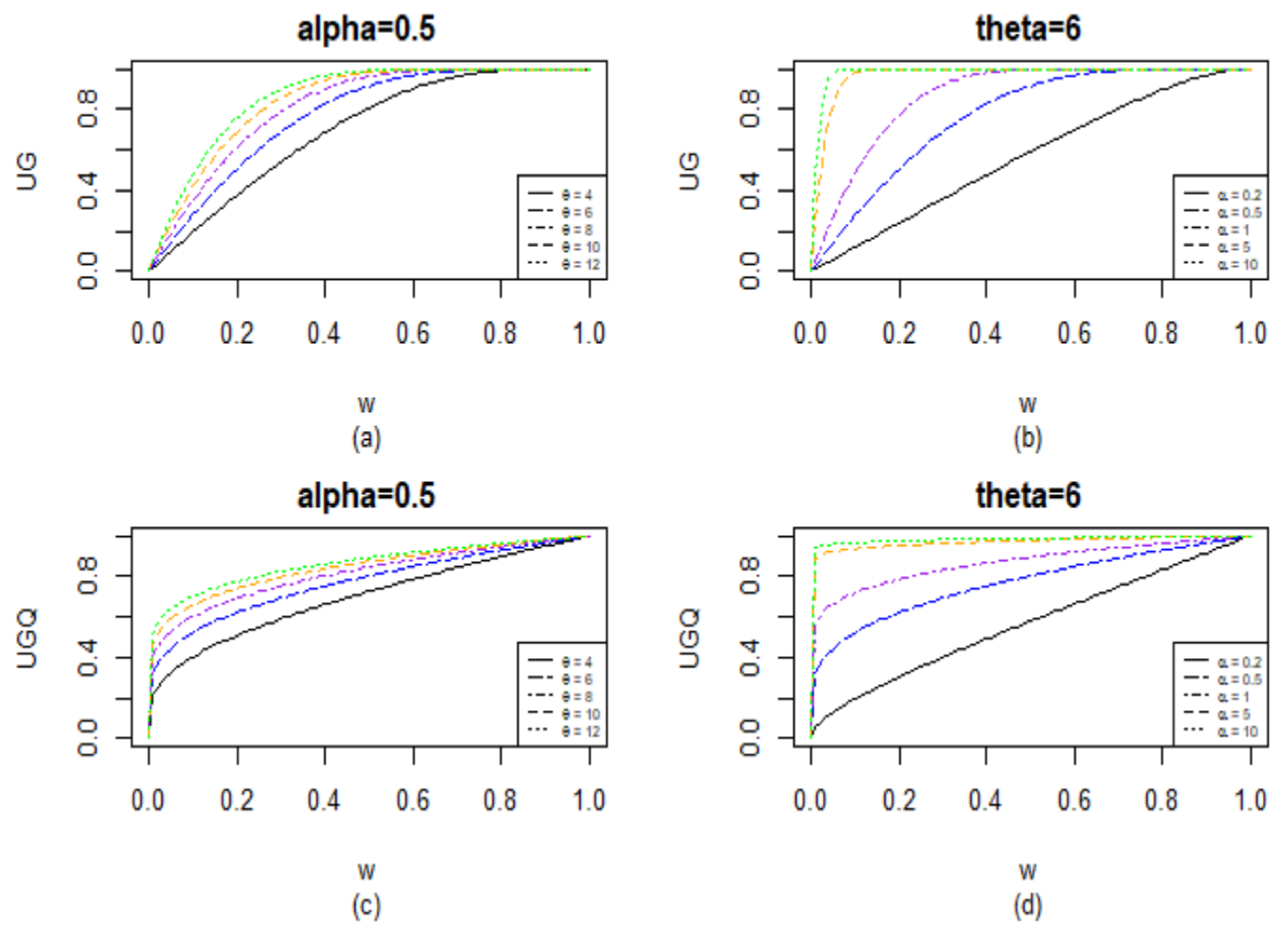
Figure 1 shows how the two new distortions UG and UGQ behave at varying $\theta$ and $\alpha$ values. Assuming that a risk-neutral agent would not distort the survival distribution, Belles-Sampera et al. (2016) used the area under a distortion function as a measure of global risk attitude. The area under a concave curve on [0, 1] is always greater than half, and a larger area indicates a higher level of global risk-tolerant attitude.

For the UG distortion, when $\alpha =0.5,$ Graph (a) indicates that a higher level of global risk-tolerant attitude and risk aversion is associated with a larger $\theta$ value. Setting $\theta =6$ (Graph (b)), a larger $\alpha$ value corresponds to a larger level of global risk-tolerant attitude. When $\alpha =10$ and $\theta =6$, the area under the curve is close to 1, which reflects a very conservative global risk-tolerant attitude. Similarly, for the UGQ distortion, the choice of a larger $\theta$ at a fixed $\alpha$ value or a larger $\alpha$ at a fixed $\theta$ value reflects a higher level of global risk-tolerant attitude.

From (2), the derivative of the distortion $g^{\prime }\left(w\right),0<w\le 1$, i.e., the slope of the tangent line to a distortion curve at w, is the assigned weight to the loss of $S^{-1}\left(w\right)$. For example, when $\alpha =0.5$, at a small extreme survival value w, the slopes of the tangent lines to the curves increase as $\theta$ increases. That is, a greater weight is assigned to a large extreme loss as $\theta$ increases, indicating a higher level of risk aversion. One, therefore, expects to obtain a larger distortion risk measure for a larger $\theta$; see Tables 2 and 3 below

3. Examples of Distortion Risk Measures

In this section, we calculate the distortion risk measures defined in (1) for uniform, exponential, Lomax, and Weibull losses using the distortions in Table 1. The derivations of the Kumaraswamy and UEE risk measures for the exponential and Lomax losses can be found in Samanthi and Sepanski (2018).

3.1. Uniform Loss

When the loss variable is uniform over the interval $[0,2b]$, then the respective cdf and survival function are $F\left(x\right)=x/2b$ and $S\left(x\right)=1-x/2b$ for $0\le x\le 2b.$ In this case, we use the formula of $\rho =\int g\left(S\left(x\right)\right)dx$ in (1) to calculate the distortion risk measures.

The Kumaraswamy risk measure for the uniform loss is given by, with substitution $s={[(2b-x)/2b]}^{\alpha }$ or $x=2b(1-s^{1/\alpha })$,

$$\begin{array}{c}\hfill {\int }_0^{2b}1-{\left[1-{\left(\frac{2b-x}{2b}\right)}^{\alpha }\right]}^{\theta }dx=2b-{\displaystyle \frac{2b}{\alpha }}{\int }_0^1{(1-s)}^{\theta }{s}^{(1-\alpha )/\alpha }ds=2b\left[1-\frac{1}{\alpha }B\left(\theta +1,\frac{1}{\alpha }\right)\right].\end{array}$$

When $\theta =1$, the Kumaraswamy risk measure is the PH or power risk measure of $2b/(1+\alpha )$ for $0<\alpha \le 1$; see also Wang (1995).

The UEE risk measure, with substitution $s=1-{(x/2b)}^{\theta }$ or $x=2b{(1-s)}^{1/\theta }$, is given by

$$\begin{array}{c}\hfill {\int }_0^{2b}{\left[1-{\left(\frac{x}{2b}\right)}^{\theta }\right]}^{\alpha }dx=\frac{2b}{\theta }{\int }_0^1{s}^{\alpha }{\left(1-s\right)}^{1/\theta -1}ds=\frac{2b}{\theta }B\left(\alpha +1,\frac{1}{\theta }\right).\end{array}$$

For the UG distortion, with substitution $s={(x/2b)}^{-\alpha },$ the UG risk measure is given by

$$\begin{array}{c}\hfill {\int }_0^{2b}\left(1-e^{-\theta \left[{(x/2b)}^{-\alpha }-1\right]}\right)dx=2b-{\displaystyle \frac{2b}{\alpha }}{\int }_1^{\infty }{\displaystyle \frac{e^{\theta }{e}^{-\theta s}}{s^{-(1+1/\alpha )}}}dx=2b-{\displaystyle \frac{2b}{\alpha }}{e}^{\theta }E\left(1+{\displaystyle \frac{1}{\alpha }},\theta \right),\end{array}$$

where $E(a,z)={\int }_1^{\infty }{e}^{-zs}/s^{a}ds$ is the generalized exponential integral.

The UGQ distortion risk measure is, with substitution $s=1-(1/\theta )ln\left(1-x/2b\right),$

$$\begin{array}{cc}\hfill & {\int }_0^{2b}{\left[1-\frac{1}{\theta }lnS\left(x\right)\right]}^{-1/\alpha }dx={\int }_0^{2b}{\left[1-\frac{1}{\theta }ln\left(\frac{2b-x}{2b}\right)\right]}^{-1/\alpha }dx\hfill \\ \hfill & =2b\theta e^{\theta }{\int }_1^{\infty }{e}^{-\theta s}{s}^{-1/\alpha }ds=2b\theta e^{\theta }E\left({\displaystyle \frac{1}{\alpha }},\theta \right).\hfill \end{array}$$

The distortion risk measures derived for a uniform loss on $[0,2b]$ in this section are summarized in

Table 2. Distortion risk measures for a uniform loss on $(0,2b)$.

Distortion	Parameter Space	Risk Measures
Power	$0<\alpha \le 1$	$2b\alpha /(1+\alpha )$
Dual-power	$\theta \ge 1$	$2b\theta /(\theta +1)$
Kumaraswamy	$0<\alpha \le 1,\theta \ge 1$	$2b-(2b/\alpha )B(\theta +1,1/\alpha )]$
UEE	$0<\alpha \le 1,\theta \ge 1$	$(2b/\theta )\left[B\right(\alpha +1,1/\theta \left)\right]$
UG	$\alpha >0,\theta >1+1/\alpha +1$	$2b-(2b/\alpha )e^{\theta }E(1+1/\alpha ,\theta )$
UGQ	$\alpha >0,\theta >1+1/\alpha +1$	$2b\theta e^{\theta }E(1/\alpha ,\theta )$

below. The distortion risk measures by power and dual-power distortions in Wang (1995) are special cases of the Kumaraswany risk measures. They are presented not only as a strategy for double-checking the calculations, but also due to their popularity.

3.2. Exponential Loss

When the loss variable X has an exponential distribution with mean b, the respective cdf, survival function, and their inverses are $F\left(x\right)=1-e^{-x/b}$, $S\left(x\right)=e^{-x/b}$, $F^{-1}\left(u\right)=-bln(1-u)$, and $S^{-1}\left(u\right)=-blnu$. Below, the formulas in (2) will be used and the derivative $g^{\prime }$ of each distortion in Table 1 will be required.

The Kumaraswamy risk measure for an exponential loss can also be found in Samanthi and Sepanski (2018). Briefly, from (2), it is given by, with substitution $s=u^{\alpha },$

$$\begin{array}{c}\hfill {\int }_0^1\alpha \theta (-blnu){\left(1-u^{\alpha }\right)}^{\theta -1}{u}^{\alpha -1}du=\frac{-b}{\alpha }{\int }_0^1\theta (lns){(1-s)}^{\theta -1}ds=\frac{b}{\alpha }\left[\mathsf{\Psi }(\theta +1)-\mathsf{\Psi }\left(1\right)\right],\end{array}$$

where the integral is the expected value of the logarithm of a beta variable with parameters 1 and $\theta$ and the digamma function $\mathsf{\Psi }\left(a\right)=d\mathsf{\Gamma }\left(a\right)/\mathsf{\Gamma }\left(a\right).$

Since $ln(1+s)\le s$ for $s>-1,$ the UEE distortion risk measure is

$$\begin{array}{ccc}\hfill & & {\int }_0^1{F}^{-1}\left(s\right)g^{\prime }(1-s)ds=-b\alpha \theta {\int }_0^{1}ln(1-s)s^{\theta -1}{(1-s^{\theta })}^{\alpha -1}ds\hfill \\ & & \le b\alpha \theta {\int }_0^1{s}^{\theta }{(1-s^{\theta })}^{\alpha -1}ds\le b\alpha \theta {\int }_0^1{s}^{\theta -1}{(1-s^{\theta })}^{\alpha -1}ds,\hfill \end{array}$$

(10)

which is finite for $\theta \ge 1.$ Applying the fact $ln(1-s)=-{\sum }_{k=1}^{\infty }{s}^k/k$, for $\left|s\right|<1,$ the risk measure in (10) is given by

$$\begin{array}{c}\hfill b\alpha \theta \sum _{k=1}^{\infty }\frac{1}{k}{\int }_0^1{s}^{k+\theta -1}{(1-s^{\theta })}^{\alpha -1}ds=b\alpha \sum _{k=1}^{\infty }\frac{1}{k}{\int }_0^1{t}^{k/\theta }{(1-t)}^{\alpha -1}dt=b\alpha \sum _{k=1}^{\infty }\frac{1}{k}B\left(1+\frac{k}{\theta },\alpha \right).\end{array}$$

When $\theta =1,$ ${\sum }_{k=1}^{\infty }B\left(1+k,\alpha \right)/k={\sum }_{k=1}^{\infty }{\int }_0^1{s}^k{(1-s)}^{\alpha -1}/kds={\int }_1^{0}ln(1-s){(1-s)}^{\alpha -1}ds=\left[{(1-s)}^{\alpha }(1-\alpha ln(1-s))\right]/{\alpha }^2){\mid }_1^0=1/{\alpha }^2$ and the UEE risk measure is reduced to the power risk measure. When $\alpha =1,$ ${\sum }_{k=1}^{\infty }B\left(1+k/\theta ,1\right)/k={\sum }_{k=1}^{\infty }(1/k)\theta /(\theta +k)={\sum }_{k=1}^{\infty }[1/k-1/(\theta +k)]=\mathsf{\Psi }(\theta +1)-\mathsf{\Psi }\left(1\right)$; see https://en.wikipedia.org/wiki/Digamma_function, (accessed on 6 October 2021).

The UG risk measure is given by, with substitution $s=t^{-\alpha }\in (\infty ,1)$,

$$\begin{array}{cc}\hfill & b\alpha \theta e^{\theta }{\int }_0^{1}ln(1-t)e^{-\theta t^{-\alpha }}{t}^{-\alpha -1}dt=b\alpha \theta e^{\theta }\sum _{k=1}^{\infty }{\int }_0^1\frac{t^{k-\alpha -1}}{k}{e}^{-\theta t^{-\alpha }}dt\hfill \\ \hfill & =b\theta e^{\theta }\sum _1^{\infty }\frac{1}{k}{\int }_1^{\infty }{s}^{-k/\alpha }{e}^{-\theta s}ds=b\theta e^{\theta }\sum _1^{\infty }\frac{1}{k}E\left(\frac{k}{\alpha },\theta \right),\hfill \end{array}$$

where E is the generalized exponential integral. It is shown in Section 3.4 that this UG exponential risk measure as a special case of UG Weibull risk measures being finite.

The UGQ risk measure using the formula $\rho =\int g\left(S\right(x\left)\right)dx$ is

$$\begin{array}{c}\hfill {\int }_0^{\infty }{\left[1-{\displaystyle \frac{1}{\theta }}ln\left(e^{-x/b}\right)\right]}^{-1/\alpha }dx={\int }_0^{\infty }{\left(1+{\displaystyle \frac{x}{b\theta }}\right)}^{-1/\alpha }dx.\end{array}$$

When $\alpha \ge 1,$ the risk measure is not finite. When $0<\alpha <1$, it is $b\alpha \theta /(1-\alpha )$.

Table 3. Distortion risk measures for an exponential loss with mean b.

Distortion	Parameter Space	Risks Measure
Power	$0<\alpha \le 1$	$b/\alpha$
Dual Power	$\theta \ge 1$	$b\left[\mathsf{\Psi }\right(\theta +1)-\mathsf{\Psi }(1\left)\right]$
Kumaraswamy	$0<\alpha \le 1,\theta \ge 1$	$(b/\alpha )\left[\mathsf{\Psi }\right(\theta +1)-\mathsf{\Psi }(1\left)\right]$
UEE	$0<\alpha \le 1,\theta \ge 1$	$b\alpha {\sum }_{k=1}^{\infty }(1/k)B(1+(k/\theta ),\alpha )$
UG	$\alpha >0,\theta >\frac{1}{\alpha }+1$	$b\theta e^{\theta }{\sum }_{k=1}^{\infty }(1/k)E(k/\alpha ,\theta )$
UGQ	$\alpha >0,\theta >\frac{1}{\alpha }+1$	$b\alpha \theta /(1-\alpha )$ if $0<\alpha <1;$ undefined if $\alpha \ge 1$

summarizes the distortion risk measures for an exponential loss with mean $b.$ It is obvious that a larger mean of b results in a larger distortion risk measure. As the distortion parameter $\theta$ increases, the resulting distortion risk measure increases. As indicated in Figure 1, a larger $\theta$ represents a higher level of risk aversion. The effects of the distortion parameter $\alpha$ do not have the same pattern across the distortions considered in Table 3. For example, for $0\le \alpha <1$, as $\alpha$ increases, the power and Kumaraswamy risk measures for exponential losses decrease while the UGQ exponential risk measure increases.

For an exponential loss with a mean of 50, the 3D Figure 2 displays the UEE and UG distorted risk measures involving the sum of an infinite series, numerically computed using R, with the parameter values $\alpha$ and $\theta$ in their respective admissible spaces. The plots for the UEE and UG risk measures allow us to gain better insight into the effect of the parameters on the risk measures. A larger $\theta$ value appears to yield a larger UEE or UG exponential risk measure, which is not at all transparent by examining the formulas. The effect of increasing $\alpha$ seems less dramatic when $alaha$ is large for the UG distortion.

3.3. Lomax Loss

The cdf, survival function, and their inverses, with parameters $a>0$ and $b>0$, of a Lomax loss variable X are given by, for $x>0$ and $0<u\le 1,$

$$\begin{array}{cc}\hfill F\left(x\right)=1-{\left(\frac{b}{b+x}\right)}^a,& F^{-1}\left(u\right)=b\left[{(1-u)}^{-1/a}-1\right],\\ \hfill S\left(x\right)={\left(\frac{b}{b+x}\right)}^a,& S^{-1}\left(u\right)=b\left[u^{-1/a}-1\right],\end{array}$$

(11)

respectively. The Lomax loss has a mean of $b/(a-1)$. The calculations of the Kumaraswamy and UEE distortion risk measures for a Lomax loss are shown in Samanthi and Sepanski (2018).

By (2), (11), and with substitution $s=u^{-\alpha }$, the UG distortion risk measure for a Lomax loss is

$$\begin{array}{cc}\hfill & {\int }_0^1{F}^{-1}\left(u\right)g^{\prime }(1-u)dt=b\alpha \theta {\int }_0^1\left[{(1-u)}^{-1/a}-1\right]u^{-\alpha -1}{e}^{-\theta (u^{-\alpha }-1)}du\hfill \\ \hfill & =b\alpha \theta {\int }_0^1\sum _{k=1}^{\infty }{(-1)}^k{u}^{k-\alpha -1}{e}^{-\theta (u^{-\alpha }-1)}du\hfill \\ \hfill & =b\theta e^{\theta }{\int }_1^{\infty }\sum _{k=1}^{\infty }{(-1)}^k\left(\genfrac{}{}{0pt}{}{-1/a}{k}\right)s^{-k/\alpha }{e}^{-\theta s}ds=b\theta e^{\theta }\sum _{k=1}^{\infty }{(-1)}^k\left(\genfrac{}{}{0pt}{}{-1/a}{k}\right)E\left({\displaystyle \frac{k}{\alpha }},\theta \right),\hfill \end{array}$$

where E is the generalized exponential integral, since ${(1-u)}^{-1/a}={\sum }_{k=0}^{\infty }{(-1)}^k{u}^k\left(\genfrac{}{}{0pt}{}{-1/a}{k}\right).$

The UGQ distortion risk measure for a Lomax loss is given by

$$\begin{array}{c}\hfill {\int }_0^{\infty }{\left[1-\frac{lnS\left(x\right)}{\theta }\right]}^{-1/\alpha }dx={\int }_0^{\infty }{\left[1-\frac{a}{\theta }ln\left(\frac{b}{b+x}\right)\right]}^{-1/\alpha }dx.\end{array}$$

(12)

With substitution $s=1-\left(a/\theta \right)ln\left(b/(b+x)\right)$, $s>1$, the integral in (12) is

$$\begin{array}{c}\hfill {\displaystyle \frac{b\theta }{a}}{e}^{-\theta /a}{\int }_1^{\infty }{s}^{-1/\alpha }{e}^{\theta s/a}ds={\displaystyle \frac{b\theta }{a}}{e}^{-\theta /a}{\int }_1^{\infty }{a}^{1-1/\alpha }{t}^{-1/\alpha }{e}^{\theta t}dt\end{array}$$

Note that, by L’Hopital’s rule, for $0<\alpha \le 1,$

$$\begin{array}{c}\hfill \underset{t\to \infty }{lim}{\displaystyle \frac{e^{\theta t}}{t^{1/\alpha }}}=\underset{t\to \infty }{lim}{\left({\displaystyle \frac{e^{\alpha \theta t}}{t}}\right)}^{1/\alpha }=\underset{t\to \infty }{lim}{\left({\displaystyle \frac{\alpha \theta e^{\alpha \theta t}}{1}}\right)}^{1/\alpha }=\infty \end{array}$$

Therefore, the risk measure in (12) is not well defined.

The mean of a Lomax loss increases as a decreases and b increases. Intuitively, one expects the parameters a and b to have the same effect on the distortion risk measures, which can be verified from the formulas except for the UEE distortion in

Table 4. Distortion risk measures for a Lomax loss with parameters $(a,b)$.

Distortion	Parameter Space	Risk Measures
Power	$0<\alpha \le 1$	$b/(a\alpha -1),a\alpha \ne 1$
Dual Power	$\theta \ge 1$	$b\theta \left[B\right(1-1/a,\theta )-B(1,\theta \left)\right]$
Kumaraswamy	$0<\alpha \le 1,\theta \ge 1$	$b\theta \left[B\right(1-1/\left(a\alpha \right),\theta )-B(1,\theta \left)\right],a\alpha \ne 1$
UEE	$0<\alpha \le 1,\theta \ge 1$	${\sum }_{k=0}^{\infty }\left(\genfrac{}{}{0pt}{}{\theta }{k}\right){(-1)}^k[1+{\sum }_{i=1}^{\infty }\left(\genfrac{}{}{0pt}{}{\alpha k}{i}\right)\frac{{(-1)}^{i}b}{ia-1}]$
UG	$\alpha >0,\theta >\frac{1}{\alpha }+1$	$b\theta e^{\theta }{\sum }_{k=1}^{\infty }{(-1)}^k\left(\genfrac{}{}{0pt}{}{-1/a}{k}\right)E\left(k/\alpha ,\theta \right)$
UGQ	$\alpha >0,\theta >\frac{1}{\alpha }+1$	Undefined

. Varying the $\alpha$ and $\theta$ values, we plot the UEE and UG risk measures for a Lomax loss with a mean of 50 with $(a,b)=(12.61,580.40)$ in Figure 3. The figure shows that the UEE Lomax risk measure increases as $\theta$ increases and $\alpha$ decreases and that the UG Lomax risk measure increases as $\theta$ or $\alpha$ increases. When the risk aversion indicator $\theta$ increases, all distorted risk measures increase.

3.4. Weibull Loss

When the loss variable X follows a Weibull distribution, its respective cdf and survival function are $F\left(x\right)=1-e^{-x^c/b}$ and $S\left(x\right)=e^{-x^c/b}$. It has a mean of $b^{1/c}\mathsf{\Gamma }(1+1/c).$ The quantile function is $F^{-1}\left(u\right)={\left[-bln\left(1-u\right)\right]}^{1/c}$ for $0<u<1.$ The hazard rate function of the Weibull distribution with parameters b and c is $(c/b)x^{(c-1)}$. It is a decreasing function when $c<1$, marking a heavy-tailed distribution, and increasing when $c>1$, marking a light-tailed distribution. The characteristics of its hazard function make the Weibull distribution an adequate model for a variety of applications, such as weather forecasting, insurance modeling, and financial risk analysis; see Frees (2018).

For the Weibull loss, the Kumaraswamy risk measure is defined to be

$$\begin{array}{cc}\hfill & {\int }_0^{\infty }1-{\left[1-{\left(S\left(x\right)\right)}^{\alpha }\right]}^{\theta }dx={\int }_0^{\infty }1-{\left[1-e^{-\alpha x^c/b}\right]}^{\theta }dx\le \theta {\int }_0^{\infty }{e}^{-\alpha x^c/b}dx,\hfill \end{array}$$

since Bernoulli’s inequality states that ${(1+t)}^r\ge 1+rt$ for $t\ge -1$ and $r\ge 1,$ and ${(1+t)}^r$$\le 1+rt$ for $t\ge -1$ and $0\le r\le 1.$ With a substitution of $x^c$, the integral ${\int }_0^{\infty }{e}^{-\alpha x^c/b}dx=\mathsf{\Gamma }(1/c){(b/\alpha )}^{1/c}/c$ for $c>0$ and is finite. Thus, the Kumaraswamy distortion risk measure for a Weibull loss is finite. By the binomial expansion of ${(1+t)}^a={\sum }_{k=1}^{\infty }\left(\genfrac{}{}{0pt}{}{a}{k}\right)t^k$ for $\left|t\right|<1,$ the risk measure is given by

$$\begin{array}{c}\hfill \sum _{k=1}^{\infty }{\int }_0^{\infty }\left(\genfrac{}{}{0pt}{}{\theta }{k}\right){(-1)}^k{\left[e^{-\alpha x^c/b}\right]}^{k}dx=\frac{1}{c}\sum _{k=1}^{\infty }\left(\genfrac{}{}{0pt}{}{\theta }{k}\right){(-1)}^k{\left(\frac{\alpha k}{b}\right)}^{-1/c}\mathsf{\Gamma }\left(\frac{1}{c}\right).\end{array}$$

When $\alpha =1$, we obtain the dual-power distortion risk measure given by

$$\begin{array}{c}\hfill \frac{1}{c}\sum _{k=1}^{\infty }\left(\genfrac{}{}{0pt}{}{\theta }{k}\right){(-1)}^k{\left(\frac{k}{b}\right)}^{-1/c}\mathsf{\Gamma }\left(\frac{1}{c}\right).\end{array}$$

(13)

When $c=1,$ the Weibull loss reduces to the exponential loss. Using the Newton series for the digamma function, the risk measure in (13) is equal to

$$\begin{array}{c}\hfill b\sum _{k=1}^{\infty }\left(\genfrac{}{}{0pt}{}{\theta }{k}\right){(-1)}^k{k}^{-1}\mathsf{\Gamma }\left(1\right)=b\left[\mathsf{\Psi }(\theta +1)-\mathsf{\Psi }\left(1\right)\right],\end{array}$$

which coincides with the result for the exponential loss in Table 3.

Since $0<1-e^{-x^c/b}<1$ for $x>0$ and ${(1-e^{-x^c/b})}^{\alpha }\ge {(1-e^{-x^c/b})}^{\theta }$ for the admissible parameter space of $0<\alpha \le 1,\theta \ge 1,$ and by applying Bernoulli’s inequality, the UEE risk measure for the Weibull loss, we obtain that

$$\begin{array}{cc}\hfill & {\int }_0^{\infty }{\left[1-{(1-e^{-x^c/b})}^{\theta }\right]}^{\alpha }dx\le {\int }_0^{\infty }{\left[1-{(1-e^{-x^c/b})}^{\theta }\right]}^{\alpha }dx\le {\theta }^{\alpha }{\int }_0^{\infty }{e}^{-\alpha x^c/b}dx\hfill \end{array}$$

which is finite.

The UG Weibull risk measure has no closed form and needs to be computed numerically. Below, we show that the UG Weibull risk measure is finite. It is defined to be

$$\begin{array}{cc}& {\int }_0^{\infty }1-e^{-\theta \left[{(1-e^{-x^c/b})}^{-\alpha }-1\right]}dx\\ & ={\int }_0^{1}1-e^{-\theta \left[{(1-e^{-x^c/b})}^{-\alpha }-1\right]}dx+{\int }_1^{\infty }1-e^{-\theta \left[{(1-e^{-x^c/b})}^{-\alpha }-1\right]}dx\\ \hfill & \le {\int }_0^{1}1-e^{-\theta \left[{(1-e^{-x^c/b})}^{-\alpha }-1\right]}dx+{\int }_1^{\infty }\theta \left[{(1-e^{-x^c/b})}^{-\alpha }-1\right]dx=A_1+\theta A_2\end{array}$$

(14)

since $e^t\ge 1+t$ or $1-e^t\le -t$ by the Taylor series. The integrand in $A_1$ is bounded on the unit interval; therefore, $A_1$ in (14) is finite. Let $z=1-e^{-1/b}.$ With the substitution $t=(1-e^{-x^c/b})\in (1-e^{-1/b},1)$ and $x={[-bln(1-t)]}^{1/c}$ for $1<x<\infty$ and using integration by parts, $A_2$ is given by

$$\begin{array}{cc}\hfill & (t^{-\alpha }-1){\left[-bln(1-t)\right]}^{1/c}{|}_{t=z}^1+\alpha b^{1/c}{\int }_z^1{t}^{-\alpha -1}{\left[-ln(1-t)\right]}^{1/c}dt\\ & =b^{1/c}{lim}_{t=1}(t^{-\alpha }-1){[-ln(1-t)]}^{1/c}+1-z^{-\alpha }+\alpha b^{1/c}{\int }_z^1{t}^{-\alpha -1}{\left[-ln(1-t)\right]}^{1/c}dt.\end{array}$$

(15)

The limit term in (15) can be shown to be 0 by repeatedly applying L’Hopital’s rule and limit laws. By the Cauchy–Schwarz inequality for integrals, we obtain that

$$\begin{array}{c}\hfill {\int }_z^1{t}^{-\alpha -1}{\left[-ln(1-t)\right]}^{1/c}dt\le {\left({\int }_z^1{t}^{-2(\alpha +1)}dt\right)}^{1/2}{\left({\int }_z^1{\left[-ln(1-t)\right]}^{2/c}dt\right)}^{1/2}\end{array}$$

(16)

By substitution $s=-ln(1-t)$, $t\in [1-e^{-1/b},1)$ and $s\in [1/b,\infty ),$

$$\begin{array}{c}\hfill {\int }_{1-e^{-1/b}}^1{\left[-ln(1-t)\right]}^{2/c}dt={\int }_{1/b}^{\infty }{s}^{2/c}{e}^{-s}ds<\mathsf{\Gamma }(2/c+1).\end{array}$$

(17)

Combining (14), (15), (16), and (17), we conclude that the UG Weibull risk measure is finite.

The UGQ risk measure for the Weibull loss is given by, with substitution $s={[1+x^c/\left(\theta b\right)]}^{-1},$

$$\begin{array}{cc}\hfill & {\int }_0^{\infty }{\left[-{\theta }^{-1}lnS\left(x\right)+1\right]}^{-1/\alpha }dx={\int }_0^{\infty }{\left(1+\theta b{x}^c\right)}^{-1/\alpha }dx\\ & =\frac{1}{c}{\left(\theta b\right)}^{1/c}{\int }_0^1{\left(1-s\right)}^{1/c-1}{s}^{1/\alpha -1/c-1}ds=\frac{1}{c}{\left(\theta b\right)}^{1/c}B\left(\frac{1}{\alpha }-\frac{1}{c},\frac{1}{c}\right).\end{array}$$

(18)

The beta function is only well defined if $1/\alpha -1/c$ is positive, i.e., if $\alpha <c$. When $c=1$ and $\alpha <1$, (18) is equal to $\theta b\alpha /(1-\alpha );$ see Table 3.

From

Table 5. Distortion risk measures for a Weibull loss with parameters b and c.

Distortion	Parameter Space	Risk Measures
Power	$\theta \ge 1$	$\mathsf{\Gamma }(1+1/c){\left(b\theta \right)}^{1/c}$
Dual-Power	$\theta \ge 1$	$\mathsf{\Gamma }(1+1/c)b^{1/c}{\sum }_{k=1}^{\infty }\left(\genfrac{}{}{0pt}{}{\theta }{k}\right){(-1)}^k{\left(k\right)}^{-1/c}$
Kumaraswamy	$0<\alpha \le 1,\theta >1$	$\mathsf{\Gamma }(1+1/c)b^{1/c}{\alpha }^{-1/c}{\sum }_{k=1}^{\infty }\left(\genfrac{}{}{0pt}{}{\theta }{k}\right){(-1)}^k{k}^{-1/c}$
UEE	$0<\alpha \le 1,\theta \ge 1$	$\mathsf{\Gamma }(1+1/c)b^{1/c}{\sum }_{k=0}^{\infty }\left(\genfrac{}{}{0pt}{}{\alpha }{k}\right){(-1)}^k{\sum }_{i=0}^{\infty }\left(\genfrac{}{}{0pt}{}{\theta k}{i}\right){(-1)}^i{i}^{-1/c}$
UG	$\alpha >0,\theta >\frac{1}{\alpha }+1$	Finite
UGQ	$\alpha >0,\theta >\frac{1}{\alpha }+1$	$(1/c){\left(\theta b\right)}^{1/c}B(1/\alpha -1/c,1/c),\alpha <c$

, the power distortion churns out a risk measure that is ${\theta }^{1/c}$ times the mean loss. For a heavy-tailed Weibull loss with $c<1$, the distorted risk measure would increase by a higher magnitude than the case with $c>1$. By Table 5 and Figure 4, the distortion risk measure increases as $\theta$ increases or $\alpha$ decreases for the UEE and Kumaraswany distortions.

4. Numerical Analyses and Estimation

In this section, we numerically compute distortion risk measures for uniform, exponential, Lomax, and Weibull losses. Note that the parameter $\theta$ in Table 1 assumes values of at least 1. We then propose a non-parametric, plug-in estimator for the distortion risk measure and conducted simulations to compare the proposed estimator with the empirical L-estimator in (4).

4.1. Numerical Results for Distortion Risk Measures

The loss distributions considered are uniform on the interval $(0,100)$, exponential with mean 50, Lomax with parameters $(12.61,580.40),$ and Weibull with parameters $(5,c=0.50)$ and $(412.20,c=1.50).$ The loss distribution parameters were selected so that all loss distributions had a mean of 50. We fixed the mean value of the loss distributions and inspected how distortion risk measures vary with the tailedness, measured by the kurtosis, of a loss distribution. A normal distribution has a kurtosis of 3 and an exponential distribution of 6. The Lomax loss parameters were chosen to have a kurtosis of 12. For the Weibull loss, we used $c=0.5$ and $c=1.5$, corresponding to heavy-tailed and light-tailed distributions with kurtoses of 84.72 and 1.39, respectively. Note that the UGQ distorted Lomax risk measures are not well-defined; see Table 4. The VaR and CTE values at various percentile levels for each loss distribution are reported as benchmark comparisons and can provide insights into the right tails of the loss random variables under study. They are supplied in

Table 6. VaR and CTE values at levels of 0.25, 0.5, 0.75, 0.95, and 0.99 for uniform $(0,100)$, exponential $\left(0.02\right)$, Lomax $(12.61,580.40)$, Weibull $(5,0.5)$, and Weibull $(412.20,1.5)$ losses.

		Level
Loss		0.25	0.5	0.75	0.95	0.99
Uniform	VaR	25	50	75	95	99
	CTE	62.6	75	87.5	97.5	99.5
Exponential	VaR	14.38	34.66	69.31	149.79	230.26
	CTE	64.38	84.66	119.31	199.79	280.26
Lomax	VaR	13.39	32.80	67.45	155.64	255.84
	CTE	64.54	85.61	123.25	219.04	327.87
Weibull (5, 0.5)	VaR	2.07	12.01	48.05	224.36	530.19
	CTE	66.45	96.67	167.36	424.15	810.45
Weibull (412.20, 1.5)	VaR	24.14	43.38	68.86	115.10	153.31
	CTE	62.01	76.23	97.32	138.63	174.22

. The risk premium, defined as the difference between the premium, e.g., the CTE, and the expected value, is larger for a loss with a heavier tailedness.

Table 7. The beta, Kumaraswamy, UEE risk measures for uniform $(0,100)$, exponential $\left(0.02\right)$, Lomax $(12.61,580.40)$, Weibull $(5,0.5)$, and Weibull $(412.20,1.5)$ losses.

		Beta			Kumaraswamy			UEE
		$\alpha$			$\alpha$			$\alpha$
Loss	$\theta$	0.25	0.5	1	0.25	0.5	1	0.25	0.5	1
Uniform	1	80	66.67	50	80	66.67	50	80	66.67	50
	2	88.89	80	66.67	93.33	83.33	66.67	87.4	78.54	66.67
	10	97.56	95.24	90.91	99.90	98.48	90.91	96.76	94.36	90.91
Exponential	1	200	100	50	200	100	50	196.78	99.97	50
	2	240	133.33	75	300	150	75	227.27	128.5	75
	10	325.26	213.33	146.45	585.79	292.9	146.45	302.62	203.32	146.65
Lomax	1	269.64	109.41	50	269.64	109.41	50	209.30	109.41	50
	2	327.22	147.91	76.02	429.87	168.82	76.02	313.05	142.23	76.02
	10	460.15	247.46	155.91	1034.72	363.65	155.49	431.41	234.36	155.49
Weibull (5, 0.5)	1	800.00	200.00	50.00	800	200	50	799.30	200.00	50.00
	2	992.00	288.89	87.50	1400	350	26.91	945.45	274.58	87.50
	10	1485.30	575.95	253.22	4051.45	1012.86	253.22	1373.67	532.94	253.22
Weibull (412.20, 1.5)	1	125.99	79.37	50.00	125.99	79.37	50.00	125.99	79.37	50.00
	2	146.72	99.98	68.50	172.61	108.74	68.50	142.34	97.22	68.50
	10	185.73	141.92	111.28	280.41	176.65	111.28	178.52	137.52	111.28

tabulates the beta, Kumaraswamy, and UEE risk measures for the losses examined in Section 3 and

Table 8. UG and UGQ risk measures for uniform $(0,100)$, exponential $\left(0.02\right)$, Lomax $(12.61,580.40)$ and Weibull $(5,0.5)$, and Weibull $(412.20,1.5)$ losses.

		UG				UGQ
		$\alpha$				$\alpha$
Loss	$\theta$	0.25	0.5	1	5	0.25	0.5	1	5
Uniform	5	58.10	73.94	85.21	96.69	58.10	79.94	85.21	96.09
	10	72.78	84.37	91.56	98.20	72.78	84.37	91.56	98.20
	15	79.76	88.79	94.08	98.76	79.76	88.79	94.08	98.76
	20	83.88	91.26	95.44	99.05	83.88	91.26	95.44	99.05
Exponential	5	59.76	87.14	117.85	195.02	83.33	250	1252.69	16,897.55
	10	85.64	116.10	148.57	227.24	166.67	493.38	2162.13	19,249.5
	15	102.56	134.26	167.40	246.63	250.00	735.20	2944.07	20,729.93
	20	115.16	147.54	181.03	260.56	333.33	973.87	3644.30	21,821.35
Lomax	5	59.92	88.74	122.41	214.18	-	-	-	-
	10	87.24	120.58	157.79	256.06	-	-	-	-
	15	105.62	144.22	180.29	282.28	-	-	-	-
	20	119.60	156.67	196.99	301.59	-	-	-	-
Weibull (c = 0.5)	5	61.88	106.77	172.66	416.78	208.33	5022.05	180,021.20	-
	10	105.13	169.86	257.64	554.89	833.33	16,688.58	-	-
	15	139.51	217.08	318.39	647.58	1875	33,135.06	-	-
Weibull (c = 1.5)	5	58.03	77.02	95.73	135.91	67.69	130.45	330.07	2279.65
	10	75.87	94.59	112.54	150.81	107.46	206.83	499.95	2572.00
	15	86.47	104.79	122.24	159.43	140.81	270.65	462.31	2752.00
	20	93.96	111.93	129.01	165.47	170.58	327.39	744.17	2882.70

the UG and UGQ risk measures for some admissible parameter values. The dash notation in Table 8 connotes that the resulting risk measure is not finite for UGQ Lomax risk or not well-defined due to the lack of admissibility. The beta and Kumaraswamy distortions both have the power and dual-power distortions as their special cases when $\theta =1$ or $\alpha =1;$ therefore, they are expected to have the same risk measures in theses cases. While this conclusion seems trivial, we computed them to possibly detect programming errors.

The distortion risk measures in Table 7 and Table 8 appear to increase as $\theta$ increases, as shown in the previous section. As $\alpha$ increases, the resulting risk measures appear to decrease for the beta, Kumaraswamy, and UEE distortions and increase for the UG and UGQ distortions if well-defined. The loss distributions with a larger kurtosis or tailedness are more sensitive to the distortion in the sense that the distortion will yield a larger risk measure. The UGQ distortion measures seem to be more sensitive than the other distortions to the loss kurtosis. As we can see for the exponential and Weibull ($c=0.5$) losses, they can be much larger than the VaR and CTE. Both the VaR and CTE values of the four loss distributions fall in between the ranges of the distortion measures produced by the beta, Kumaraswamy, UEE, and UG distortions presented, which may be seen as an indication that those distortions have practicability.

4.2. Estimation of Distortion Risk Measures

Instead of (2), we considered the equation in (1) such that $\rho ={\int }_0^{\infty }x{g}^{\prime }\left(S\left(x\right)\right)f\left(x\right)dx=E\left[X{g}^{\prime }\left(S\left(X\right)\right)\right],$ the expected value of the function $X{g}^{\prime }\left(S\left(X\right)\right)$. An intuitive estimator of an expected value is the sample mean. Let $\widehat{F}\left(x\right)={\sum }_{j=1}^{n}I(X_j\le x)/n$ denote the empirical cdf. Then, the survival function $S\left(X\right)$ can be estimated by

$$\widehat{S}\left(x\right)=1-\widehat{F}\left(x\right)=\sum _{j=1}^{n}I(X_j>x)/n.$$

The proposed plug-in estimator is given by

$$\begin{array}{c}\hfill {\widehat{\rho }}_p={\displaystyle \frac{1}{n}}\sum _{i=1}^n{X}_i{g}^{\prime }\left(\widehat{S}\left(X_i\right)\right).\end{array}$$

No parametric assumptions were made about the underlying loss distribution.

Below, we employed simulations for the time being to preliminarily investigate the behaviors of the proposed estimator and compare it with the empirical L-estimator in (4) for the exponential loss and the Lomax losses with parameters of 5 and 200, both with a mean of 50. The exponential distribution had a kurtosis of 6 and the Lomax distribution a kurtosis of 70.8. Five-hundred simulations were run for each of sample sizes $n=50,100,500,$ and 1000 for various distortions. For each distortion, we ran them for three pairs of admissible $\alpha$ and $\theta$ values. The true theoretical distortion risk measures, the sample mean, the bias defined as the difference between the sample mean and the theoretical risk measure, and the standard deviations of estimates from the 500 simulations are displayed in

Table 9. Sample means, biases and standard deviations in parentheses of L-estimates and plug-in estimates from 500 simulations for exponential loss with mean 50.

Distortion	L-estimate	Plug-in		L-estimate	Plug-in		L-estimate	Plug-in
Beta (0.5, 3)	153.33	153.33	Beta (0.5, 6)	187.82	187.82	Beta (1, 3)	91.67	91.67
$n=50$	133.92 (24.45)	134.28 (24.51)	$n=50$	159.65 (32.04)	159.61 (33.06)	$n=50$	90.53 (12.79)	90.51 (13.16)
mean bias	−19.42	−19.00		−28.17	−28.21		−1.14	−1.16
$n=100$	140.11 (19.52)	142.36 (18.98)	$n=100$	168.60 (25.88)	166.54 (24.38)	$n=100$	91.28 (9.92)	91.30 (4.54)
mean bias	−13.22	−12.65		−19.22	−21.28		−0.38	−0.29
$n=500$	147.08 (10.50)	149.63 (9.89)	$n=500$	178.81 (14.23)	180.29 (14.59)	$n=500$	91.40 (4.56)	91.44 (4.54)
mean bias	−6.26	−5.97		−9.01	−7.53		−0.27	−0.25
$n=1000$	148.94 (7.62)	152.67 (6.90)	$n=1000$	181.48 (10.40)	183.32 (8.52)	$n=1000$	91.54 (3.01)	91.92 (2.67)
mean bias	−4.39	−0.66		−6.34	−3.5		−0.13	0.25
Kumar (0.5, 3)	183.33	183.33	Kumar (0.5, 6)	245	245	Kumar (1, 3)	91.67	91.67
$n=50$	153.52 (30.90)	149.16 (28.54)	$n=50$	189.24 (44.53)	189.21 (40.51)	$n=50$	90.53 (12.19)	92.77 (13.10)
mean bias	−29.81	−34.17		−55.76	−55.79		−1.14	1.1
$n=100$	162.68 (25.22)	166.45 (21.42)	$n=100$	205.39 (37.99)	211.48 (33.99)	$n=100$	91.28 (9.92)	92.41 (10.04)
mean bias	−20.65	−16.88		−39.61	−33.52		−0.39	0.74
$n=500$	173.56 (14.22)	180.52 (13.96)	$n=500$	226.17 (23.12)	230.59 (21.46)	$n=500$	91.40 (4.56)	91.63 (4.58)
mean bias	−9.77	−2.81		−18.83	−14.41		−0.27	−0.04
$n=1000$	176.74 (11.19)	181.33 (10.01)	$n=1000$	231.92 (18.99)	234.67 (17.93)	$n=1000$	91.71 (3.04)	91.82 (3.04)
mean bias	−6.59	−2.00		−13.08	−10.33		0.04	0.15
UEE (0.5, 3):	146.51	146.51	UEE (0.5, 6)	178.78	178.78	UEE (1, 3)	91.67	91.67
$n=50$	128.66 (23.05)	130.89 (21.63)	$n=50$	153.37 (29.94)	154.26 (27.26)	$n=50$	90.53 (12.79)	92.77 (13.09)
mean bias	−17.85	−15.62		−25.41	−24.52		−1.14	1.10
$n=100$	134.37 (18.37)	139.65 (17.32)	$n=100$	161.48 (24.08)	168.94 (22.45)	$n=100$	91.28 (9.92)	92.41 (10.04)
mean bias	−12.14	−6.86		−17.30	−9.84		−0.39	0.74
$n=500$	140.78 (9.83)	143.20 (8.66)	$n=500$	170.69 (13.15)	174.27 (12.59)	$n=500$	91.40 (4.56)	91.63 (4.58)
mean bias	−5.73	−3.31		−8.09	−4.51		−0.27	−0.04
$n=1000$	142.67 (7.48)	144.89 (6.21)	$n=1000$	173.43 (10.12)	176.53 (10.05)	$n=1000$	91.71 (3.04)	91.82 (3.04)
mean bias	−3.75	−1.62		−5.35	−2.25		−0.04	0.15
UG (1, 3)	96.90	96.90	UG (1, 6)	125.71	125.71	UG (6, 3)	181.26	181.26
$n=50$	95.75 (13.60)	97.76 (13.85)	$n=50$	122.56 (19.12)	129.45 (20.08)	$n=50$	171.92 (33.96)	201.23 (39.16)
mean bias	−1.15	0.86		−3.15	3.74		−9.34	19.97
$n=100$	96.51 (10.53)	97.51 (10.63)	$n=100$	124.56 (14.73)	127.86 (15.10)	$n=100$	177.20 (26.07)	191.95 (28.05)
mean bias	−0.39	0.61		−1.15	2.15		−4.06	10.66
$n=500$	96.63 (4.84)	96.83 (4.85)	$n=500$	125.18 (6.84)	125.83 (6.57)	$n=500$	179.86 (12.19)	182.81 (12.38)
mean bias	−0.27	−0.07		−0.53	0.12		−1.4	1.55
$n=1000$	96.94 (3.22)	97.04 (3.22)	$n=1000$	125.70 (4.54)	126.03 (4.55)	$n=1000$	180.89 (8.34)	182.37 (8.41)
mean bias	0.04	0.14		−0.01	0.32		−0.37	1.11
UGQ (0.5, 4)	200	200	UGQ (0.5, 8)	400	400	UGQ (0.25, 8)	133.33	133.33
$n=50$	106.04 (20.39)	111.20 (21.23)	$n=50$	143.76 (32.37)	146.12 (29.49)	$n=50$	98.67 (17.67)	99.11 (18.4)
mean bias	−93.96	−88.80		−256.24	−254.88		−34.66	−34.22
$n=100$	113.58 (17.54)	114.67 (18.96)	$n=100$	158.15 (29.37)	169.43 (26.40)	$n=100$	104.20 (14.66)	110.76 (15.00)
mean bias	−86.42	−85.33		−241.85	−230.57		−29.13	−22.57
$n=500$	126.15 (12.16)	130.04 (11.99)	$n=500$	184.32 (22.95)	193.44 (19.98)	$n=500$	112.40 (9.09)	123.13 (7.99)
mean bias	−73.85	−69.96		−215.69	206.56		−20.94	−10.20
$n=1000$	130.88 (1128)	133.81 (10.99)	$n=1000$	194.36 (22.41)	196.27 (20.02)	$n=1000$	115.33 (7.87)	125.04 (6.82)
mean bias	−69.12	−66.19		−205.64	−203.73		−18.00	−8.29

and

Table 10. Sample means, biases and standard deviations parentheses of L-estimates and plug-in estimates from 500 simulations for Lomax loss with parameters (5, 200).

Distortion	L-estimate	Plug-in		L-estimate	Plug-in		L-estimate	Plug-in
Beta (0.5, 3)	218.06	218.06	Beta (0.5, 6)	281.53	281.53	Beta (1, 3)	97.62	97.62
$n=50$	156.33 (50.52)	160.01 (51.77)	$n=50$	192.52 (68.41)	191.22 (67.13)	$n=50$	94.78 (20.66)	93.63 (20.10)
mean bias	−61.73	−58.05		−89.01	−90.31		−3.14	−3.85
$n=100$	179.79 (37.62)	178.99 (38.82)	$n=100$	214.40 (51.68)	215.30 (50.96)	$n=100$	97.20 (13.71)	97.17 (13.45)
mean bias	−46.27	−39.07		−67.13	−66.23		−0.42	−0.45
$n=500$	188.99 (26.26)	190.43 (27.11)	$n=500$	239.49 (36.98)	240.15 (35.49)	$n=500$	97.45 (6.63)	97.43 (6.06)
mean bias	−29.07	−27.63		−42.05	−41.38		−0.17	−0.19
$n=1000$	193.66 (21.78)	194.59 (21.74)	$n=1000$	246.79 (33.98)	248.15 (32.94)	$n=1000$	97.42 (5.04)	97.58 (4.55)
mean bias	−24.40	−23.47		−34.74	−33.38		−0.20	−0.04
Kumar (0.5, 3)	280.77	280.77	Kumar (0.5, 6)	422.11	422.11	Kumar (1, 3)	97.62	97.62
$n=50$	185.03 (66.45)	185.16 (33.83)	$n=50$	239.38 (100.43)	242.69 (55.64)	$n=50$	94.48 (20.66)	96.76 (21.13)
mean bias	−95.74	−95.61		−182.73	−179.42		−3.14	−0.86
$n=100$	207.45 (51.01)	217.63 (28.73)	$n=100$	278.24 (81.00)	281.56 (49.53)	$n=100$	97.20 (13.71)	97.68 (6.65)
mean bias	−73.32	−63.14		−143.87	−140.55		−0.42	0.06
$n=500$	234.50 (37.86)	240.52 (24.08)	$n=500$	330.43 (65.85)	340.23 (28.26)	$n=500$	97.45 (6.63)	97.68 (6.65)
mean bias	−46.27	−40.25		−91.68	−81.88		−0.17	0.06
$n=1000$	242.66 (33.26)	249.74 (22.81)	$n=1000$	346.24 (60.48)	353.64 (24.77)	$n=1000$	97.57 (4.52)	97.58 (4.50)
mean bias	−38.11	−31.03		−75.87	−68.47		−0.05	−0.04
UEE (0.5, 3):	206.21	206.21	UEE (0.5, 6)	263.84	263.84	UEE (1, 3)	97.62	97.62
$n=50$	149.17 (47.26)	155.63 (46.39)	$n=50$	183.26 (63.31)	184.81 (60.52)	$n=50$	94.48 (20.66)	96.76 (21.13)
mean bias	−57.04	−50.58		−80.58	−79.03		−3.14	−0.86
$n=100$	163.51 (35.10)	159.99 (33.47)	$n=100$	203.19 (47.58)	206.34 (49.08)	$n=100$	97.20 (13.71)	98.36 (13.86)
mean bias	−42.7	−22.97		−38.03	−31.26		−0.14	0.06
$n=500$	179.37 (24.38)	183.24 (22.31)	$n=500$	225.81 (33.75)	232.58 (34.25)	$n=500$	97.48 (6.63)	97.68 (6.65)
mean bias	−26.84	−22.97		−38.03	−31.26		−0.14	0.06
$n=1000$	184.16 (20.70)	186.47 (19.05)	$n=1000$	232.63 (28.91)	239.43 (28.93)	$n=1000$	97.58 (4.52)	97.58 (4.50)
mean bias	−22.05	−19.74		−31.21	−24.41		−0.04	−0.04
UG (1, 3)	103	103	UG (1, 6)	141.23	141.23	UG (6, 3)	226	226
$n=50$	99.84 (20.69)	101.79 (22.03)	$n=50$	135.03 (31.33)	142.03 (35.59)	$n=50$	207.08 (62.65)	241.23 (79.61)
mean bias	−3.16	−1.21		−6.20	0.8		−18.92	15.23
$n=100$	102.47 (15.29)	103.63 (14.51)	$n=100$	139.25 (23.97)	143.50 (23.03)	$n=100$	217.35 (50.29)	237.62 (50.37)
mean bias	−0.53	0.63		−1.98	2.27		−8.65	11.62
$n=500$	102.67 (6.78)	103.64 (6.95)	$n=500$	140.38 (10.84)	141.44 (11.16)	$n=500$	223.12 (24.09)	227.67 (24.57)
mean bias	−0.33	0.64		−0.85	0.21		−2.88	1.67
$n=1000$	102.89 (4.77)	102.89 (4.78)	$n=1000$	140.92 (7.76)	141.56 (7.67)	$n=1000$	224.91 (17.55)	228.35 (17.05)
mean bias	−0.11	−0.11		−0.31	0.33		−1.09	2.35

.

As one would expect, the bias and standard deviation decreased as the sample size increased in Table 9 and Table 10. As seen in the previous section, as $\theta$ increased, the resulting distortion risk measure increased, so were the biases and standard deviations of the L-estimator and plug-in estimators. A distortion of a loss distribution with a larger kurtosis would result in a larger risk measure and also a larger bias and standard deviation in the two estimators. When the sample size was 500 and 1000, in general, the proposed plug-in estimates appeared to perform slightly better than the L-estimates in terms of the bias and standard deviation. Based on the results from the sample size of 1000, both the L-estimator and plug-in estimators seemed to be consistent for the distortions with parameter values of $\alpha =1$ and $\theta =3$. Though the proposed plug-in estimator had smaller biases in the majority of the cases, both estimators performed poorly in estimating the UGQ risk measures for the exponential loss.

5. Concluding Remarks

The framework employed in the paper was motivated by the fact that a cumulative distribution function with unit interval support is a distortion function. It utilizes an exponential transformation of a non-negative random variable, whose distribution function is named the generating distribution, to a random variable with a support of the unit interval. There are other functions, for instance $1/(1+x),$ that can transform a non-negative random variable into a variable with unit interval support.

There are numerous candidates for the role of the generating distribution. The generating distributions employed here included the exponentiated exponential and Gompertz distributions. The proposed framework opens the door to a world of new distortion functions. We demonstrated that the framework also produces some existing well-known distortions, e.g., power and dual-power distortions. We developed two new distortion functions and derived admissible spaces on the parameters so that the resulting distortion risk measures were coherent. The distortion risk measures for uniform, exponential, Lomax, and Weibull losses were computed. The effects of the distortion parameters on the risk measures and risk tolerance attitudes were examined by graphs and closed-form expressions of risk measures. As Wang and Xu (2023) pointed out, there has been little discussion on which distortion risk measures at hand should be chosen. It would be of great interest to further explore how to tune the parameters to better reflect or approximate decision-maker’s risk preferences and various risk attitudes.

We proposed a plug-in estimator for the distortion risk measure and ran simulations to compare it with the empirical L-estimator in Jones and Zitikis (2003). It appeared that the plug-in estimator, just like the empirical L-estimator, suffered biases when losses followed heavy-tailed or Pareto-liked distributions. Kim (2010) showed that, when the distortion function is concave, L-estimates of distortion risk measures are negatively biased, and the bias can be corrected through the bootstrapping for a continuous loss distribution. The negative biases in the L-estimates were demonstrated in our simulation results. While this is not the case for the proposed plug-in estimate, the simulation results indicated that the proposed plug-in estimates seemed to also perform poorly for heavy-tailed losses. Brahimi et al. (2012) proposed an alternative estimators of L-functionals for heavy-tailed losses by means of extreme value theory and established their asymptotic normality. Abdelaziz (2015) established a new estimator using an approximation of the tail of the loss distribution. The asymptotic distribution of the proposed plug-in estimator will be investigated first, and bias correction estimators may then ensue in the future.

Kim (2010) proposed to correct the bias through bootstrapping for a continuous loss distribution. Brahimi et al. (2012) proposed alternative estimators of L-functionals for heavy-tailed losses by means of extreme value theory and established their asymptotic normality. Abdelaziz (2015) established a new estimator using an approximation of the tail of the loss distribution. The asymptotic distribution of the proposed plug-in estimator will be investigated first, and bias correction estimators may then ensue in the future.