Assessing the Impact of Credit Risk on Equity Options via Information Contents and Compound Options

Abstract

This work aims to develop a measure of how much credit risk is priced into equity options. Such a measure appears particularly appealing when applied to a portfolio of equity options, as it allows for the factoring in of firm-specific default dynamics, thus producing a comparable statistic across different equities. As a matter of fact, comparing options written on different equities based on their moneyness does offer much guidance in understanding which option offers a better hedging against default. Our newly-introduced measure aims to fulfil this gap: it allows us to rank options written on different names based on the amount of default risk they carry, incorporating firm-specific characteristics such as leverage and asset risk. After having computed this measure using data from the US market, several empirical tests confirm the economic intuition of puts being more sensitive to changes in the default risk as well as a good integration of the CDS and option markets. We further document cross-sectional sectorial differences based on the industry the companies operate in. Moreover, we show that this newly-introduced measure displays forecasting power in explaining future changes in the skew of long-term maturity options.

1. Introduction

Markets for both stock options and credit derivatives have experienced a significant growth in the last decades. Along with the rapid growth, academics have started investigating a possible link between stock option implied volatilities and credit default swaps (CDS) spreads: when a company experiences credit-rating downgrades, its equity inevitably drops by a sizable amount and, therefore, the prices of the options written on the company’s equity react as well. As a result, the possibility of default induces negative skewness in the probability distribution of stock returns. This negative skewness is manifested in the relative pricing of stock options across different strikes: when the Black and Scholes (1973) implied volatility is plotted against moneyness at fixed maturities, the slope of the graph is positively related to the risk-neutral skewness of the stock return distribution. This phenomenon is commonly referred in the literature as the leverage effect.

Anecdotal evidence suggests that major investment bank are more and more focused on issuing derivative contracts such as equity default swaps1 or more structured products2 for covering downside risk. These derivatives are written on to the firm’s equity rather than the firm’s debt, and their building blocks are mostly equity options (vanilla or barrier). The reason for using equity rather than debt for such purposes lie in a larger liquidity and immediate reaction in prices of equity prices rather than (traded and nontraded) debt instruments.

The relation between default risk and option prices is studied extensively in the literature. Early research shows that the pricing of ordinary options differs from the pricing of options with default risk (Johnson and Stulz 1987; Hull and White 1995; Jarrow and Turnbull 1995). More recent studies look at the relation between credit spreads and option prices (Cremers et al. 2008a; Carr and Wu 2010; Andreou 2015; Geske et al. 2016; Culp et al. 2018).

The aim of this work is to study the impact of credit risk on equity options. The proposed framework also allows for the exploitation of the overlapping information on the market risk and the credit risk of a company to provide better identification of the dynamics of the stock return variance and default events, and how these impact equity option prices. Ultimately, this allows not only to measure the impact of credit risk on equity options and but also to light on the mechanism leading to future movements of the option skew due to credit-related events.

The first works to point out a possible effect of leverage and credit risk on equity option are Black (1976) and Christie (1982). They both argue that the possibility by the company of defaulting on its obligations can induce negative skewness in the company’s return distribution. This manifests when the implied volatility is plotted against a measure of moneyness and exhibits a decreasing pattern for increasing strike prices (the so-called negative volatility skew) rather than a flat line. The skew is often observed in the region where the implied volatility is estimated using out-of-the-money put options, being the latter intrinsically affected the most by credit risk. More recent empirical works, such as Collin-Dufresne et al. (2001), Elton et al. (2001), Cremers et al. (2008a, 2008b), and Cao et al. (2010), show that CDS and bond spreads are positively correlated with both stock option implied volatility levels and the skew of the implied volatility plotted against moneyness. Also, Campbell and Taksler (2003), and  Ericsson et al. (2009) document a link between bond spreads and equity historical volatility. At the aggregate level, similar results hold for sovereign CDS spreads (Carr and Wu 2007), and credit default swap index (CDX) spreads and synthetic collateralised debt obligations (CDOs) on the same index (Collin-Dufresne et al. 2012).

The relative pricing of equity- and debt-related derivatives instruments has been mainly explored using reduced-form models of default in the literature. Carr and Linetsky (2006), Mendoza-Arriaga et al. (2010) and Carr and Wu (2010) develop joint frameworks of valuation for credit-sensitive derivatives contracts and equity options. Their estimations highlight the interaction between market risk (return variance) and credit risk (default arrival) in pricing stock options and credit default swaps. They also point out the need of developing future models that integrate both markets, rather than having separate valuation models. This work tries to bridge this gap providing a unique structural valuation framework where both the price of CDSs and options written on the same reference entity are driven by a unique state variable, namely the firm’s asset value, which ultimately determines the default event properties.

On the other side of the spectrum, the use of a structural model for jointly modelling credit and equity derivative contracts has not been exhaustively explored. With the exception of Toft and Prucyk (1997), which built on the Leland (1994) model to document the effect of leverage on the pricing of options, and Hull et al. (2004), which develop a new calibration methodology based on options to implement the Merton (1974) model, there have not been significant attempts to develop structural models of default able to transmit the company’s credit risk to the pricing of equity options. In this work instead, the firm is allowed to issue multiple bonds with different maturities, thus removing the restriction on perpetual debt (as in Leland 1994) or a unique zero-coupon bond (as in Merton 1974). The work of Geske et al. (2016) moves towards this direction whilst investigating capital structure effects on the pricing of equity options. However, their work does not measure the extent to which leverage and credit risk impact the pricing of options which is assessed in this paper. Also, they focus on call options only, which intuitively should be affected by credit risk the least, whilst here both call and put options are taken into consideration.

Regarding the selection of data to infer default probabilities, CDS spreads are used rather than bond prices. This is motivated by the fact that CDS spreads constitute a more direct and clean signal for the underlying default risk. In fact, CDS spreads provide relatively pure pricing of the default event of the underlying entity as they are typically traded on standardised terms: unlike bonds, CDSs have a constant maturity, the underlying instrument is always par valued, they concentrate liquidity in one instrument, and are not affected by different taxation regimes. Moreover, many corporate bonds are bought by investors who simply hold them to maturity, and the secondary market liquidity is therefore often poor.3 CDS contracts instead allow investors to implement trading strategies to hedge credit risk over a longer period of time at a known cost. In addition, as shown by Blanco et al. (2005), CDS spreads tend to respond more quickly than bond spreads to changes in credit conditions in the short run.

This work also connects with the findings in Carr and Wu (2011, 2017). More specifically, Carr and Wu (2011) show that under suitable assumptions the price of equity put options struck deepest out-of-the-money (DOOM) is entirely driven by the default possibility of the reference entity. Also, they show that the contract values of credit-sensitive instruments and put options share similar magnitudes and show strong co-movements. On the other hand, Carr and Wu (2017) is a crucial piece of research in interpreting and assessing the extent to which results on the volatility skew obtained herein could be driven by factors other than the leverage effect. In their article, the authors identify three different channels able to generate the negative volatility skew documented in equity options. They show that the option skew can be driven, as expected, by increasing leverage, but also by volatility feedback and self-exciting market disruptions.

In terms of the modelling of equity options, the theory employed here is based on Merton (1974), Geske (1977), and Geske (1979) where the equity is considered as a contingent claim on the firm’s value. Here, as the reference firm has issued more than one bond, equity turns into a n-fold compound option (where n is the number of bonds outstanding). To the best of our knowledge, this is the first work that uses the theory of n-fold compound options for pricing vanilla equity options.

Based on the model predictions and using a novel calibration technique, a measure of impact of credit risk is introduced. The effect of credit-related event is further investigated in the relative pricing of call and put options, showing that indeed put options price the credit risk implied by the credit spread. The ability of this new measure to forecast future movement in the option skew is then tested. Finally, the model allows us to show how the estimation of the implied volatility á la Black–Scholes tend to average out the effect of credit risk over the moneyness space, leading to potential biases when applied for risk management purposes.

The rest of the paper is structured as follows: Section 2 introduces the value of the equity as a n-fold compound option and extend the pricing to equity options; Section 3 introduces the novel measure of impact of credit risk on option contracts; in Section 4 we describe the dataset, the construction of the required variables and the calibration methodology employed to estimate the unobservable asset value and volatility; Section 5 is devoted to several empirical tests which assess the different impact of credit risk on calls and puts, cross-sectional differences based on the sector the companies operate in, and the ability of our measure to forecast future movements in the option skew. Finally, Section 6 concludes.

2. Firm’s Claims as Compound Options

The structural model of default used to price the price equity, debt and options written on equity is the model introduced in Maglione (2022), which is an extension of Merton (1974) and Geske (1977). Before discussing how to price option within the chosen compound option model, we briefly review the main features of the structural model of default.

In terms of general assumptions, we take a reference firm financed with n bonds and equity. Both liabilities receive of stream og cash flow in the form of coupons and dividends which are paid at a continuous rate. According to the indenture of the bonds: (1) the firm promises to repay each bond, with face value $F_i$, to the bondholders at known times $t_i\in (t_0,t_n]$, $i\in I:=\left\{1,\dots ,n\right\}$; (2) in case of default, the bondholders immediately take over the company and the shareholders receive nothing; (3) the firm cannot issue any senior or equivalent rank claims on the firm nor do share repurchases before $t_n$. Usual assumptions in terms of transaction cost, taxes, bid/ask spreads, short-selling and indivisibility of assets apply.4

For convenience of notation, set $t_0:=0$ and denote the generic payoff at time $t_i$ as $X_{t_i}:=X_i$. Let V, S and D represent the firm’s assets, equity and debt respectively. According to the structural approach and the Modigliani-Miller theorem, both equity and debt are function of the firm’s assets and not vice versa (Merton 1977). Also, we fix a filtered probability space $(\Omega ,\mathcal{F},\mathbb{F},\mathbb{P})$ and assume no-arbitrage conditions in the economy and the existence of a equivalent martingale probability measure $\mathbb{Q}$. Furthermore, since we assume a flat term structure of the risk-free rate at $r>0$, this equivalent martingale measure coincides with the risk-neutral measure.

Below, we provide a sketch of the main features of the compound option model of default. For a more in-depth analysis of this model, more details are found in Maglione (2022) in which the model was firstly introduced.

Default is defined as the first time the firm is unable to issue new equity to repay the bond due at time $t_i$, i.e.,

$$\tau :=\underset{i\in I}{inf}\left\{t_i:S_i^{★}\left(V\right)<F_i\right\},$$

(1)

where $S_i^{★}\left(V\right)$ is the continuation value of equity.5 As equity is a function of the assets of the firm, the same event can be defined in the asset value space6: for each value of equity which triggers default corresponds only one value of the firm assets, namely ${\overline{V}}_i$ at time $t_i$, which implies (1), that is

$$\tau =\underset{i\in I}{inf}\left\{t_i:V_i<{\overline{V}}_i\right\}.$$

Within this framework, the present value of the equity can be obtained using risk-neutral valuation as the $\mathbb{Q}$-expectation of its terminal payoffs. Since the payoff of the firm’s equity at $t_i\in [0,t_n]$, can be expressed as

$$S_n\left(V\right)=V_n{\mathbb{1}}_{\tau >t_n}-\sum _{k=i+1}^n{e}^{r(t_n-t_k)}{F}_k{\mathbb{1}}_{\tau >t_k},$$

(2)

and, assuming a geometric Brownian motion on the asset process

$$d{V}_t=\left(r-\varpi \right)V_{t}dt+{\sigma }_V{V}_{t}d{W}_t^{\mathbb{Q}},$$

(3)

where $\varpi$ is the continuously compounded payout rate, ${\sigma }_V$ the instantaneous volatility of the assets, and $W_t^{\mathbb{Q}}$ a $\mathbb{Q}$-standard Brownian motion, the today’s equity price can be expressed in terms of multivariate Gaussian integrals, i.e.,

$$\begin{array}{cc}\hfill S_0\left(V\right)& =e^{-\varpi t_n}{V}_0{\Phi }_n\left({\mathbf{d}}_{\mathbf{1}};{\Gamma }_n\right)-{\displaystyle \sum _{k=1}^n}{e}^{-r{t}_k}{F}_k{\Phi }_k\left({\mathbf{d}}_{\mathbf{2},k};{\Gamma }_k\right),\hfill \end{array}$$

(4)

where ${\mathbf{d}}_{\mathbf{1}}:={\left(d_{1,i}\right)}_{1\le i\le n}$ and ${\mathbf{d}}_{\mathbf{2},k}={\left(d_{1,i}-{\sigma }_V\sqrt{t_i}\right)}_{1\le i\le k}$ with

$$d_{1,i}=\frac{ln\left(V_0/{\overline{V}}_i\right)+\left(r-\varpi +{\sigma }_V^2/2\right)t_i}{{\sigma }_V\sqrt{t_i}},{\Gamma }_k=\left(\begin{array}{ccccc}1& \sqrt{\frac{t_1}{t_2}}& \sqrt{\frac{t_1}{t_3}}& \cdots & \sqrt{\frac{t_1}{t_k}}\\ & 1& \sqrt{\frac{t_2}{t_3}}& \cdots & \sqrt{\frac{t_2}{t_k}}\\ \cdots & \cdots & \cdots & \cdots & \cdots \\ & & & 1& \sqrt{\frac{t_{k-1}}{t_k}}\\ & & & & 1\end{array}\right),$$

(5)

and ${\Phi }_k\left(\mathbf{x};{\Gamma }_k\right)$ the multivariate CDF at $\mathbf{x}\in {\mathbb{R}}^k$ of a standard normal random vector with correlation matrix ${\Gamma }_k$. Notice that, if $n=1$ and $\varpi =0$, the model coincides with the Merton’s model.

Call and Put Equity Options as a $(n+1)$–Fold Compound Options on Asset Value

Intuitively, as equity is an n–fold compound option, vanilla options are $(n+1)$–fold compound options on the firm’s assets. Consider an European option with maturity $T\in \left(t_i,t_{i+1}\right)$, with $0\le t_i<t_{i+1}\le t_n$, and strike price K written on the firm’s equity. If the company is allowed to default at any $t_i$, the generic terminal payoff of the option is

$$P_T^{\left(\xi \right)}=\xi \left(S_T\left(V\right){\mathbb{1}}_{\left\{\tau >T\right\}}-K\right){\mathbb{1}}_{\left\{\xi S_T\left(V\right)\ge \xi K\right\}},$$

(6)

where $\xi$ is a binary variable taking values $+1$ (respectively $-1$) in the case in which the option is a call (respectively a put), ${\mathbb{1}}_{\left\{\xi S_T\left(V\right)\ge \xi K\right\}}$ determines the condition for the option to expire in-the-money, and ${\mathbb{1}}_{\left\{\tau >T\right\}}\equiv {\mathbb{1}}_{\left\{\tau >t_i\right\}}$ is the condition to accounts for the possibility of the firm to defaulted before the maturity of the option (i.e., vulnerability). The possibility for the company to default after the maturity of the option is already accounted in the value of $S_T\left(V\right)$. In case the company defaults before the option maturity (that is the first indicator function is zero) the firm’s equity drops to zero.7

Under risk-neutral valuation, the present value of the option is given by

$$P_0^{\left(\xi \right)}=e^{-rT}{\mathbb{E}}^{\mathbb{Q}}\left(P_T^{\left(\xi \right)}\right).$$

The event of the option expiring in-the-money, $\left\{\xi S_T\left(V\right)\right.$$\left.\ge \xi K\right\}$, can be redefined as the event $\left\{\xi V_T\ge \xi {\overline{V}}_K\right\}$, where ${\overline{V}}_K$ is nothing but the value of the assets corresponding to the equity value that makes the option expire in-the-money.

Defining the events ${\mathcal{V}}_{i,k}:={\bigcap }_{h=i+1}^k\left\{V_h\ge {\overline{V}}_h\right\}$ and ${\mathcal{V}}_T^{\left(\xi \right)}:=\left\{\xi V_T\ge \xi {\overline{V}}_K\right\}$, with ${\mathcal{V}}_k\equiv {\mathcal{V}}_{0,k}$, for $k\in I$, the value of the option can be written as

$$P_{0,\xi }=\xi e^{-rT}\left[{\mathbb{E}}^{\mathbb{Q}}\left(S_T\left(V\right){\mathbb{1}}_{{\mathcal{V}}_i\cap {\mathcal{V}}_T^{\left(\xi \right)}}\right)-K\mathbb{Q}\left({\mathcal{V}}_T^{\left(\xi \right)}\right)\right],$$

where, the value of the equity at the maturity of the option is given by

$$\begin{array}{cc}\hfill S_T\left(V\right)& =e^{-r\left(t_n-T\right)}{\mathbb{E}}_T^{\mathbb{Q}}\left(V_n{\mathbb{1}}_{{\mathcal{V}}_{i,n}}\right)-\sum _{k=i+1}^n{e}^{-r\left(t_k-T\right)}{F}_k{\mathbb{E}}_T^{\mathbb{Q}}\left({\mathbb{1}}_{{\mathcal{V}}_{i,k}}\right).\hfill \end{array}$$

Being ${\mathbb{1}}_{{\mathcal{V}}_i\cap {\mathcal{V}}_T^{\xi }}$${\mathcal{F}}_T$-measurable, and applying the law of iterated expectations, it follows

$$\begin{array}{cc}\hfill P_0^{\left(\xi \right)}& =\xi \left[e^{-r{t}_n}{\mathbb{E}}^{\mathbb{Q}}\left(V_n{\mathbb{1}}_{{\mathcal{V}}_n\cap {\mathcal{V}}_T^{\left(\xi \right)}}\right)-\sum _{k=i+1}^n{e}^{-r{t}_k}{F}_k\mathbb{Q}\left({\mathcal{V}}_k\cap {\mathcal{V}}_T^{\left(\xi \right)}\right)-e^{rT}K\mathbb{Q}\left({\mathcal{V}}_T^{\left(\xi \right)}\right)\right].\hfill \end{array}$$

Using (again) the result Geske (1977) on multivariate Gaussian integrals, the price of the option can be expressed as

$$P_0^{\left(\xi \right)}=\xi \left[e^{-\varpi t_n}{V}_0{\Phi }_{n+1}\left({\mathbf{d}}_{\mathbf{1}}^{\left(\xi \right)};{\Gamma }_{n+1}^{\left(\xi \right)}\right)-\sum _{k=i+1}^n{e}^{-r{t}_k}{F}_k{\Phi }_{k+1}\left({\mathbf{d}}_{\mathbf{2},k+1}^{\left(\xi \right)};{\Gamma }_{k+1}^{\left(\xi \right)}\right)-e^{-rT}K\Phi \left(\xi d_{2,T}\right)\right]$$

(7)

with ${\mathbf{d}}_{\mathbf{1}}^{\left(\xi \right)}=\left({\left(d_{1,i}\right)}_{i=1}^k,\xi d_{1,T},{\left(d_{1,i}\right)}_{i=k+1}^n\right)$, ${\mathbf{d}}_{\mathbf{2},k+1}^{\left(\xi \right)}={\left(d_{1,i}^{\left(\xi \right)}-{\sigma }_V\sqrt{t_i}\right)}_{1\le i\le k+1}$, defined as in (5), and

$$d_{1,T}=\frac{ln\left(V_0/{\overline{V}}_K\right)+\left(r-\varpi +{\sigma }_V^2/2\right)T}{{\sigma }_V\sqrt{T}},{\Gamma }_{k+1}^{\left(\xi \right)}=\left(\begin{array}{cccccc}1& \sqrt{\frac{t_1}{t_2}}& \cdots & \xi \sqrt{\frac{t_1}{T}}& \cdots & \sqrt{\frac{t_1}{t_k}}\\ & 1& \cdots & \xi \sqrt{\frac{t_2}{T}}& \cdots & \sqrt{\frac{t_2}{t_k}}\\ \cdots & \cdots & \cdots & \cdots & \cdots & \cdots \\ & & & & 1& \sqrt{\frac{t_{k-1}}{t_k}}\\ & & & & & 1\end{array}\right),$$

with $d_{2,T}=d_{1,T}-{\sigma }_V\sqrt{T}$. For $\varpi =0$, $n=1$ and $t_1>T$, the formula coincides with the option price in Geske (1979).

3. Information Content Ratios as Measure of Impact of Credit Risk

In this section, a new measure of impact of credit risk on options is first introduced. In the empirical tests, we use the newly-introduced measure to asses whether call and put options display different price impacts in terms of credit risk.

In the compound option model, the option price depends on the risk-neutral probabilities

$$\mathbb{Q}\left(\tau >t_i\cap \xi S_T>\xi K\right),i\in I,$$

(8)

which compute the likelihood of the event of the firm not defaulting (up to $t_i$) and the option expiring in-the-money. Trivially, these probabilities can be factorised as

$$\underset{\mathrm{credit}\mathrm{risk}}{\underbrace{\mathbb{Q}\left(\tau >t_i\right)}}\underset{\mathrm{market}\mathrm{risk}}{\underbrace{\mathbb{Q}\left(\xi S_T>\xi K|\tau >t_i\right)}},i\in I.$$

(9)

The first factor is the probability of the firm surviving until $t_i$, whilst the second is the probability of the option expiring in-the-money conditional on the firm having not defaulted. Therefore, this decomposition rigorously disentangles the source of credit and market risk and how these reflect into option prices.

In order to turn the multiplicative functional into an additive one, instead of looking at raw probabilities, their information content8 is instead considered. Thus, the Information Content Ratio ($ICR$) for each probability is defined as

$$IC{R}_i^{\left(\xi \right)}(K,T)=\frac{log\mathbb{Q}\left(\tau >t_i\right)}{log\mathbb{Q}\left(\tau >t_i\cap \xi S_T>\xi K\right)}i\in I.$$

(10)

This represents the percentage of credit risk over the whole event of the firm surviving and the option expiring in-the-money, expressed in terms of the information content of the two events. Notice that, given a set of $K\times T$ options, there are $n\times K\times T$ Information Content Ratios.

Once these ratios are computed for all the probabilities contributing to the price of the option, they can be then aggregated in order to measure the impact of credit risk on each option contract. The Average Information Content Ratio ($AICR$) is thus defined as a weighted average of the information content ratios, that is

$$AIC{R}^{\left(\xi \right)}(K,T)=\frac{{\sum }_i{\varphi }_i·IC{R}_i^{\left(\xi \right)}(K,T)}{{\sum }_i{\varphi }_i}.$$

(11)

The weights ${\varphi }_i$ are just the present values of the bond expiring in $t_i$. Notice that if $\tau >t_i$ a.s. for all $i\in I$ (i.e., almost sure survival), then $AIC{R}_{\xi }(K,T)=0$ (i.e., no impact of credit risk on the option contract).

Interestingly, the proposed measure is linked to the entropy of the default time. In fact, changing the base of the logarithm, Equation (10) can be written as

$$IC{R}_i^{\left(\xi \right)}(K,T)={log}_{b_i}\mathbb{Q}\left(\tau >t_i\right)$$

with $b_i=\mathbb{Q}\left(\tau >t_i\cap \xi S_T>\xi K\right)$. Therefore,

$$AIC{R}^{\left(\xi \right)}(K,T)=\sum _i{\tilde{\varphi }}_i·{log}_{b_i}\mathbb{Q}\left(\tau >t_i\right)$$

with ${\tilde{\varphi }}_i={\varphi }_i/{\sum }_i{\varphi }_i$. On the other hand, the risk-neutral entropy in base $b\in (0,1)$ of the default time is defined as9

$$H_b^{\mathbb{Q}}\left(\mathrm{default}\right)=\sum _i\mathbb{Q}\left(\tau =t_i\right){log}_b\mathbb{Q}\left(\tau =t_i\right),$$

and similarly

$$H_b^{\mathbb{Q}}\left(\mathrm{survival}\right)=\sum _i\mathbb{Q}\left(\tau >t_i\right){log}_b\mathbb{Q}\left(\tau >t_i\right).$$

As long as $b_i$ is approximately constant10 and the $\mathbb{Q}\left(\tau >t_i\right)\propto {\tilde{\varphi }}_i$ (i.e., survival probabilities up to time $t_i$ are proportional to the fraction of debt at that time), then $AICR\propto H_b^{\mathbb{Q}}\left(\mathrm{survival}\right)$.

Such a measure of credit risk obtained from option quotes is particularly interesting when considered in a portfolio framework. As a matter of fact, given a set of put options written on a reference company (which hedge against downward movements of the underlying), we could simply and trivially say that the more the put option is out-of-the-money, the more the impact of credit risk on the contract. However, when considering portfolios of options written on different equities, it would be particularly challenging to say that, say, put option A on Company X is more affected by credit risk than put option B written on Company Y, even if the two options have identical moneyness. In fact, the impact of credit risk on the single option contract depends on the leverage of the company as well as the volatility of its cash-flow, which are both company-specific. This measure standardise and factors in these firm-specific effects and provides a comparable statistic to rank option contracts written on different equities. Furthermore, as shown recently by Vasquez and Xiao (2023), delta-hedged option portfolios on the companies with high default risk more attractive to investors seeking to hedge default risk and, therefore, reduces its expected return. When the firm’s default risk increases, the expected return of the delta-hedged option portfolio should decrease to reflect the change in default risk, which is indeed what they document.

4. Data and Estimation Methodology

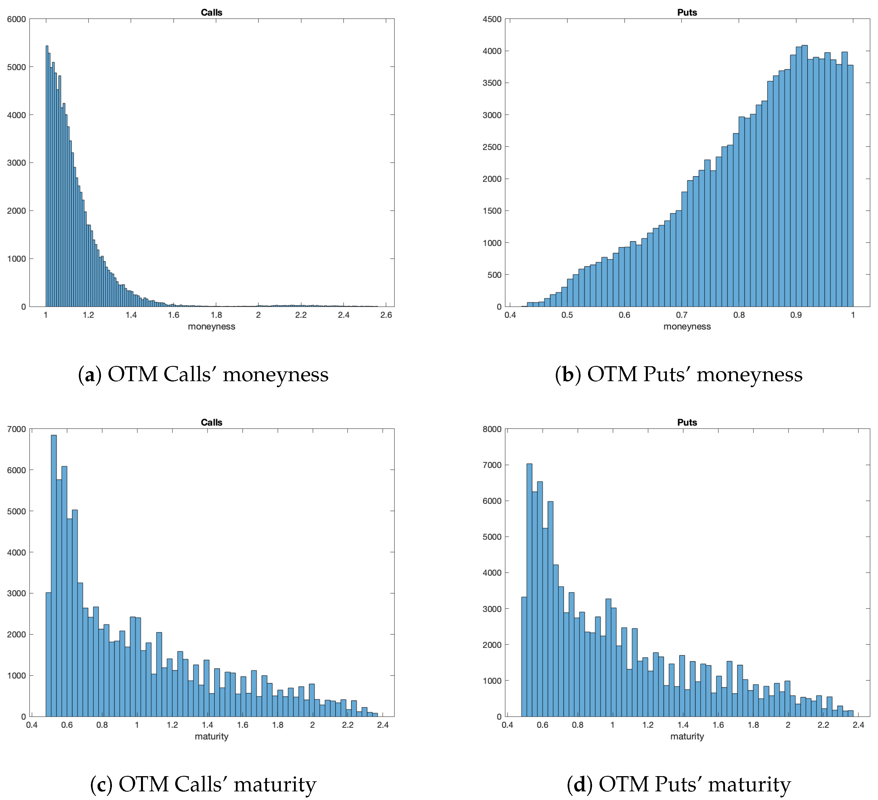
4.1. Dataset

The dataset under investigation is composed by US companies, constituents of the S&P100 during the period January 2013–December 2017. The sample period considered is due to data availability. Furthermore, we are not really focusing on picking some time-specific pattern observed over the considered years; we rather consider a sample period which does not include crises (such as the Global Financial Crisis and recent pandemic crisis) which may well affect the extent to which equity options embeds credit risk.

Regarding the cross-section of companies, firms with either preferred equity or subject to merges or acquisitions are excluded. Also, only companies for which both CDS spreads and option quotes available are included. Moreover, we consider only those companies which remained as constituents of the S&P100 during the sample period. These restrictions reduce the final sample size to 66 companies. Nevertheless, previous studies investigating the relative pricing of options and CDSs rely on much smaller samples (see for instance Hull et al. 2004; Carr and Wu 2010, 2017), both in the time-series and the cross-section.

Table 1. List of the selected companies and their SIC code.

Ticker	SIC	Division
AAPL	3663	Manufacturing
ABT	2834	Manufacturing
ACN	8742	Services
ALL	6331	Finance, Insurance and Real Estate
AMGN	2836	Manufacturing
AMZN	5961	Wholesale Trade
BA	3721	Manufacturing
BAC	6020	Finance, Insurance and Real Estate
BMY	2834	Manufacturing
C	6199	Finance, Insurance and Real Estate
CAT	3531	Manufacturing
CL	2844	Manufacturing
CMCSA	4841	Transportation, Communications, Electric, Gas and Sanitary service
COF	6141	Finance, Insurance and Real Estate
COP	1311	Mining
COST	5399	Wholesale Trade
CSCO	3576	Manufacturing
CVS	5912	Retail Trade
CVX	2911	Manufacturing
DD	2821	Manufacturing
DIS	4888	Transportation, Communications, Electric, Gas and Sanitary service
EMR	3823	Manufacturing
EXC	4911	Transportation, Communications, Electric, Gas and Sanitary service
F	3711	Manufacturing
FDX	4513	Transportation, Communications, Electric, Gas and Sanitary service
GD	3721	Manufacturing
GE	4911	Transportation, Communications, Electric, Gas and Sanitary service
HAL	1389	Mining
HD	5211	Wholesale Trade
IBM	7370	Services
INTC	3674	Manufacturing
JNJ	2834	Manufacturing
JPM	6020	Finance, Insurance and Real Estate
KO	2086	Manufacturing
LLY	2834	Manufacturing
LOW	5211	Wholesale Trade
MCD	5812	Retail Trade
MDT	3845	Manufacturing
MMM	2670	Manufacturing
MO	2111	Manufacturing
MON	5169	Retail Trade
MRK	2834	Manufacturing
MS	6211	Finance, Insurance and Real Estate
MSFT	7372	Services
ORCL	7370	Services
OXY	1311	Mining
PEP	2080	Manufacturing
PFE	2834	Manufacturing
PG	2840	Manufacturing
PM	2111	Manufacturing
RTN	3812	Manufacturing
SLB	1389	Mining
SO	4911	Transportation, Communications, Electric, Gas and Sanitary service
SPG	6798	Finance, Insurance and Real Estate
T	4812	Transportation, Communications, Electric, Gas and Sanitary service
TGT	5331	Wholesale Trade
TWX	8748	Services
TXN	3674	Manufacturing
UNH	6324	Finance, Insurance and Real Estate
UNP	4011	Transportation, Communications, Electric, Gas and Sanitary service
USB	6020	Finance, Insurance and Real Estate
UTX	3724	Manufacturing
VZ	4812	Transportation, Communications, Electric, Gas and Sanitary service
WFC	6020	Finance, Insurance and Real Estate
WMT	5331	Retail Trade
XOM	1311	Mining

displays the complete name list, alongside the SIC code of the companies.

In the same spirit of Carr and Wu (2017), the sample is further divided into four categories based on the industry/type or business: (a) Financial companies; (b) Mining, Energy and Utilities companies; (c) Manufacturing; (d) Retail, Wholesale and Services. See Figure 1 for the relative frequencies of the different sectors. A sub-sample analysis based on these groups is carried out in Section 5.1.

Data on stock prices, number of shares outstanding, dividends and the risk-free yield curve are obtained from Bloomberg. Option quotes are collected from Optionmetrics. CDS spreads are from Thompson Reuters Datastream. Information relative to the firms’ capital structures and cost of debt is gathered from Compustat and the 10-K documents.

Option quotes, CDS spreads and equity prices are observed at daily frequency. The data from Compustat on the firms’ debt is available only at quarterly frequency though. Therefore, it is assumed that the capital structure remains fixed within quarters, having only adjusted the time to maturity of the firm’s debt due to the passage of time. It appears a reasonable assumption given the empirical evidence on how often US firms decide to rebalance their capital structures (Strebulaev and Whited 2012).

Given the large amount of option data, only the most liquid OTM call and put options traded every Wednesdays with time-to-maturity greater than six months are taken into consideration. To determine the most liquid traded options, those prices whose moneyness is outside the 5th to 95th percentile range are firstly removed. Secondly, only those options with volume above their annual median are kept.

As one of the aims of this work is to study the interplay between market and credit risk, and how this is reflected into the relative pricing of derivatives contracts (options and CDSs) written on the same company, we opt for focusing on those option for which the impact of credit risk is presumably not negligible. In fact, as the database is composed by firms members of the S&P100—which should be considered as ‘safe’ companies in the short-term—it seems very unlikely that options with maturities lesser than six months would price any credit risk. This intuition is also confirmed by Cremers et al. (2008b).

The price of the option is defined as the average of the bid and ask price when both are available; the observation is removed otherwise. Finally, options with zero trading volume and negative bid-ask spread are also excluded. The final sample counts 92,879 valid call and 112,347 put options observations over 259 weeks. Figure 2 shows the options’ distribution in terms of moneyness and maturity.

One of the main disadvantage of working with equity options is that they are usually American-style. This is the case in the analysed dataset and, in order to test and implement the model, European quotes should be used. Hence, the de-Americanization procedure introduced by Carr and Wu (2010) and further tested in Burkovska et al. (2018) is applied. The aim of the de-Americanization is to find the corresponding European price (the so-called pseudo-European price) for a given American price: this is the price ought to be observed if the contract would not allow for exercising the option before maturity. In a nutshell, a binomial tree is used to price the American option. The volatility parameter, such that the squared difference between the market price and the price generated by the tree is minimised, is set as the option implied volatility. Once estimated, the pseudo-European price is found by applying the Black–Scholes formula for European options using as volatility parameter the implied volatility of the American option extracted from the tree.

In order to estimate the impact of credit risk on equity options, and verify whether the option market participants price credit risk consistently with the credit default swap market, a calibration based on equity prices, CDS spreads and option quotes is carried out. In addition, the term-structure of the firm’s debt must be known or approximated somehow. Given data availability from Compustat, we opt for clustering the firm’s debt at two points in time (i.e., $n=2$): short-term debt, maturing in one year’s time, and long-term debt, due at year ten. These are proxied by Debt in Current Liabilities (DLCQ) and Long-Term Debt–Total (DLTTQ).

Finally, the payout ratio is calculated as the weighted average cost of capital for the company. The cost of equity (i.e., dividend yield, say q) is estimated as the average dividend yield over the previous year. These data are downloaded from Bloomberg. The cost of debt is calculated as

$$c=min\left\{\frac{{\sum }_{i=1}^n{c}_i{F}_i}{F},ln\left(1+\frac{\mathtt{XINT}}{F}\right)\right\},$$

where $F={\sum }_{i=1}^n{F}_i$ and $c_i$ the continuously compounded debt payout rate. $\mathtt{XINT}$ is the Compustat variable Interest and Related Expense – Total. The individual rates $c_i$ are observed at yearly frequency and manually collected from the 10-K documents. Eventually, the payout rate is estimated every year as

$$\varpi =\frac{cF+qS}{F+S},$$

where S is the value of the equity at the beginning of the year and q the dividend yield estimated as described above.

4.2. Estimation of the Model Parameters

It is well known in the literature on structural models of default that implementing such models can be quite challenging as both asset volatility and value are unobservable. However, having obtained the price of both equity and equity options as function of the unobservable $V_0$ and ${\sigma }_V$, allows us to built a simple estimation technique to obtain these latent variables: for every option price, we solve a non-linear system of two equations (i.e., the price of equity in (4) and the option price in (7)), so to calibrate on observed market price, i.e.,

$$\left\{\begin{array}{c}\mathrm{Equity}\mathrm{price}=e^{-\varpi t_n}{V}_0{\Phi }_n\left({\mathbf{d}}_{\mathbf{1}}(V_0,{\sigma }_V);{\Gamma }_n\right)-\sum _{k=1}^n{e}^{-r{t}_k}{F}_k{\Phi }_k\left({\mathbf{d}}_{\mathbf{2},k}(V_0,{\sigma }_V);{\Gamma }_k\right)\hfill \\ \mathrm{Option}\mathrm{price}=\xi \left[e^{-\varpi t_n}{V}_0{\Phi }_{n+1}\left({\mathbf{d}}_{\mathbf{1}}^{\left(\xi \right)}(V_0,{\sigma }_V);{\Gamma }_{n+1}^{\left(\xi \right)}\right)-\sum _{k=i+1}^n{e}^{-r{t}_k}{F}_k{\Phi }_{k+1}\left({\mathbf{d}}_{\mathbf{2},k+1}^{\left(\xi \right)}(V_0,{\sigma }_V);{\Gamma }_{k+1}^{\left(\xi \right)}\right)\right.\hfill \\ \left.-e^{-rT}K\Phi \left(\xi d_{2,T}\right)\right].\hfill \end{array}\right.$$

This technique is very similar to the well-known estimation of the implied volatilities à la Black–Scholes: the value of the asset volatility, ${\sigma }_V^{★}$, and corresponding asset value, $V_0^{★}$, are found such that both the market price of equity and the option quote are matched.

The estimation of the asset volatility and value as in Section 4 allows us to compute the probabilities in (8) as well as the risk neutral probabilities of survival in (9). Hence, the probability of the option expiring in-the-money conditional upon surviving can be computed as well.

Alternatively, the risk-neutral probabilities of survival can be directly estimated in a model-free fashion using the CDSs spreads.11 The comparison of the latter with those produced by the model allows for the investigation of the model’s ability to replicate the observed term-structure of default probabilities and, indirectly, to test for the integration of the option and CDS market in terms of the pricing of default risk. In fact, the closer the probabilities obtained from option quotes are to only those estimated using CDSs, the more similar and consistent the pricing of the two derivatives contracts by the economic agents trading in the two markets are.

Finally, for each option contract the $AICR$ measure is computed. Given that every day several contracts are traded, the daily average $AICR$ is then calculated over all valid option prices. This allows us to construct a time series of a measure of the company’s credit risk which is based on option quotes. Figure 3 shows that the daily average $AICR$ calculated over calls is substantially smaller than those computed using put quotes. Furthermore, the graphs show a spike both in calls and puts at the end of 2015. This spike is likely to be caused by the fact that in 2015 the U.S. economy was so slow that several historically reliable indicators of an imminent recession were waiving red flags: Industrial Production was negative over 12 months, and retail sales growth was falling. Furthermore, the global economy was even weaker. It might well be the case that market participants, fearing an upcoming recession, priced default probabilities to a greater extent. Thus, such a shift in default outlooks has been reflected into option prices, which our measure consistently captures.

The calculation of $AICR$ can also be performed by using either the model-implied survival probabilities or those extracted from the CDSs. As $AICR$ is a linear functions of information contents in (10), the discrepancies between the $AICR$s computed using the two different sets of probabilities can shed light on the level of integration of the two markets. The next section addresses the link between the two constructions as well as the difference behaviour of put and call options in term of pricing of credit risk.

This section ends with a simple correlation analysis of the $AICR$ measure with respect to the option strike $\left(K\right)$ and time-to-maturity $\left(T\right)$. From

Table 2. Average sample correlation of $AICR$ (calls and puts, with and without having used the CDS to calibrate) with strike price (K) and maturity (T) of the options. As expected, for both calls and puts, the $AICR$ is negatively correlated with the strike price, as lower strikes proxies for default thresholds, and positively correlated with the time-to-maturity of the option, as the probability of defaulting is increasing with the time horizon. The estimates are carried out both having calculated the $AICR$s with and without the extra calibration of the risk-neutral probabilities extracted from CDSs (and are statistically equivalent). Significance levels: 10% (*), 5% (**), 1% (***).

	Calls		Puts
	$\mathit{K}$	$\mathit{T}$	$\mathit{K}$	$\mathit{T}$
Correlation (w/o CDS)	−0.0307	−0.0053	−0.0897	0.1291
p-value	0.000 ***	0.155	0.000 ***	0.000 ***
Correlation (with CDS)	−0.0723	−0.0857	−0.0751	0.1250
p-value	0.000 ***	0.000 ***	0.000 ***	0.000 ***

, the $AICR$ measure displays a statistically significant negative correlation with the strike price both for calls and puts: the lower the strike price, the higher the price of credit risk embedded in the option as expected. In addition, $AICR$s is positively correlated with the maturity of the option in the case of puts: given the probability of survival being a decreasing function of the time horizon, long-maturity options display a larger impact of credit risk. For calls, the correlation is actually negative and significant only if the $AICR$ measure is constructed using not only options, but also the probabilities of survival extracted from CDSs. These sample correlations highlight a much stronger link between credit risk and put options.

5. Empirical Tests

5.1. Cross Sectional Differences in Calls and Puts

Economic and financial intuition suggests that a different pricing behaviour of credit risk should be observed between calls and puts. As default is an event which is priced in the left tail of the equity distribution, put options as insurances against price falling should be affected more by credit-related events than calls. As a matter of fact, Carr and Wu (2011) show that, under a general class of stock price dynamics, a portfolio of two deep out-of-the-money American-style equity put options can replicate a pure credit insurance contract that pays off if and only if the company defaults prior to the option expiry.

A preliminary test is conducted on the relationship between the two measures of impact of credit risk, either constructed using option quotes only ($AICR$) or based on the option prices and CDS spreads ($AIC{R}^{\prime }$). As these measures are option-specific, the daily average for the whole set of available call and put options is calculated each week ($\overline{AICR}$ and ${\overline{AICR}}^{\prime }$, respectively). In order to estimate the risk-neutral probabilities from the CDSs, a 50% loss given default is assumed. A 50% recovery rate is consistent with the median value for senior unsecured bonds reported in Duffie and Singleton (1999) and Huang and Huang (2012). Our results are consistent and remain statistically significant under different values for the loss given default12.

The following set of unbalanced panel pooled regressions are estimated

$${\overline{AICR}}_{j,t,\xi }^{\prime }=\alpha +\beta {\overline{AICR}}_{j,t,\xi }+{\eta }_{j,t,\xi },$$

(12)

with $j\in J$, being J the set of 66 US companies, t the weekly observation, and $\xi$ the binary variable that takes value $\xi =1$ for calls and $\xi =-1$ for puts. Firstly, these regressions serve as a sanity check of the co-movements of the two measures of impact of credit risk. Secondly, the residuals ${\eta }_{j,t,\xi }$ summarise the pricing information carried by CDS in determining the $\overline{AICR}$s which is not obtainable from option prices. Results are reported in

Table 3. Estimation of regression (12). (a): Estimates of the pooled panel regression of average $AICR$ obtained from call options ($\xi =1$) and CDS regressed onto average $AICR$ obtained from call options only. Number of observations: 15,476. F-stat: 25,623.33 (p-value: 0.0000). (b): Estimates of the pooled panel regression of average $AICR$ obtained from put options ($\xi =-1$) and CDS regressed onto average $AICR$ obtained from put options only. Number of observations: 14,895. F-stat: 3321.13 (p-value: 0.0000). A sandwich estimator for panel data is used to obtain robust standard errors. Significance levels: 10% (*), 5% (**), 1% (***).

(a): ${\overline{\mathit{A}\mathit{I}\mathit{C}\mathit{R}}}^{\prime }$regressed onto$\overline{\mathit{A}\mathit{I}\mathit{C}\mathit{R}}$(both constructed on calls).
Regressand				Adj-$R^2$:	0.7416
${\overline{AICR}}_1^{\prime }$
Regressors	Coefficient	Robust Standard Error	t-stat	p-value
${\overline{AICR}}_1$	0.7936	0.0050	160.07	0.000	***
${\alpha }_1$	0.0018	0.0001	29.42	0.000	***
(b): ${\overline{AICR}}^{\prime }$ regressed onto $\overline{AICR}$ (both constructed on puts).
Regressand				Adj-$R^2$:	0.9054
${\overline{AICR}}_{-1}^{\prime }$
Regressors	Coefficient	Robust Standard Error	t-stat	p-value
${\overline{AICR}}_{-1}$	0.8357	0.0145	57.63	0.000	***
${\alpha }_{-1}$	−0.0002	0.00004	−4.21	0.000	***

. As expected, the two measures strongly co-move and the loading coefficients have the predicted sign.

The next step is assessing the different impact of credit risk on call and put options. Different measures of leverage (book leverage, model-implied market leverage estimated from options only, model-implied market leverage estimated using both options and CDSs) can be used as proxies of credit risk. In the following tests, the selected measure of leverage is the market leverage estimated using option. The final implications do not depend on the specific measure of leverage chosen and empirical results based on the other leverage measures are available upon request.

The model implied market leverage $LEV=(V-S)/S=D/S$ is then regressed onto $\overline{AICR}$ and ${\overline{AICR}}^{\prime }$ of calls and puts for each set of weekly observations.13 By common sense and the model predictions, a higher leverage should induce a larger impact of credit risk on the company’s securities. Put options are expected to show statistically significant positive loadings. More specifically, panel regressions are implemented with year- and industry-fixed effects. These are

$$\begin{array}{cc}\hfill {\overline{AICR}}_{j,t,\xi }& ={\alpha }_{\xi }+{\mu }_{i,\xi }+{\theta }_{y,\xi }+\beta {LEV}_{j,t}+{\epsilon }_{j,t,i,y,\xi }\hfill \\ \hfill {\overline{AICR}}_{j,t,\xi }^{\prime }& ={\alpha }_{\xi }^{\prime }+{\mu }_{i,\xi }^{\prime }+{\theta }_{y,\xi }^{\prime }+{\beta }^{\prime }{LEV}_{j,t}+{\epsilon }_{j,t,i,y,\xi }^{\prime }.\hfill \end{array}$$

(13)

Year-fixed effects (${\theta }_{y,\xi }$ and ${\theta }_{y,\xi }^{\prime }$, with $y=\{2013,\dots ,2017\}$) should capture the time-series variation in the volatility of the market, whilst the industry-fixed effects (${\mu }_{i,\xi }$ and ${\mu }_{i,\xi }^{\prime }$, with $i=${Financials; Mining, Energy and Utilities; Manufacturing; Retail, Wholesale and Services}) account for possible cross-sectional heterogeneity due to the sector the company operates.

The results are reported in

Table 4. Estimation of regression (13). (a): Estimates of the fixed-effects panel regression of market model-implied leverage $LEV$ onto average $AICR$ calculated over call options only. Number of observations: 15,476. (b): Estimates of the fixed-effects panel regression of market model-implied leverage $LEV$ onto average $AICR$ calculated over call options and CDSs. Number of observations: 15,476. (c): Estimates of the fixed-effects panel regression of market model-implied leverage $LEV$ onto average $AICR$ calculated over put options only. Number of observations: 14,895. (d): Estimates of the fixed-effects panel regression of market model-implied leverage $LEV$ onto average $AICR$ calculated based on put options and CDSs. Number of observations: 14,895. Standard errors are adjusted for four clusters based on industry. Significance levels: 10% (*), 5% (**), 1% (***).

(a): $\overline{\mathit{A}\mathit{I}\mathit{C}\mathit{R}}$ (constructed on calls) regressed onto $\mathit{L}\mathit{E}\mathit{V}$.
Regressand				Adj-$R^2$:	0.0309
${\overline{AICR}}_1$
Regressors	Coefficient	Robust Standard Error	t-stat	p-value
$LEV$	0.0002	0.0004	0.53	0.630
${\alpha }_1$	0.0017	0.0006	2.74	0.071	*
Industry−FE	✓
Year−FE	✓
(b): ${\overline{AICR}}^{\prime }$ (constructed on calls and CDSs) regressed onto $LEV$.
Regressand				Adj-$R^2$:	0.1120
${\overline{AICR}}_1^{\prime }$
Regressors	Coefficient	Robust Standard Error	t-stat	p-value
$LEV$	0.0066	0.0013	5.16	0.014	**
${\alpha }_1$	0.0029	0.0011	2.59	0.081	*
Industry−FE	✓
Year−FE	✓
(c): $\overline{AICR}$ (constructed on puts) regressed onto $LEV$.
Regressand				Adj-$R^2$:	0.4967
${\overline{AICR}}_{-1}$
Regressors	Coefficient	Robust Standard Error	t-stat	p-value
$LEV$	0.0253	0.0015	16.72	0.000	***
${\alpha }_{-1}$	−0.0060	0.0020	−3.07	0.054	*
Industry−FE	✓
Year−FE	✓
(d): ${\overline{AICR}}^{\prime }$ (constructed on puts and CDSs) regressed onto $LEV$.
Regressand				Adj-$R^2$:	0.5326
${\overline{AICR}}_{-1}^{\prime }$
Regressors	Coefficient	Robust Standard Error	t-stat	p-value
$LEV$	0.0236	0.0019	12.41	0.001	***
${\alpha }_{-1}$	−0.0070	0.0023	−2.98	0.059	*
Industry−FE	✓
Year−FE	✓

. Remarkably, despite the two measures of credit risk strongly co-move, in the case of call options, only ${\overline{AICR}}^{\prime }$—the measure obtained by adding the information carried by CDSs—is able to capture the credit risk of the company. Regardless, as the main effect of default on equity is to reduce its value by a sizeable amount, it is understandable that credit risk does not affect much call options. Therefore, the joint calibration on options and CDS carries extra information that, especially for call options, is relevant for capturing default risk dynamics.

To stress this point further, the following regressions

$${\eta }_{j,t,\xi }={\alpha }_{\xi }+{\mu }_{i,\xi }+{\theta }_{y,\xi }+\beta {LEV}_{j,t}+{ϵ}_{j,t,i,y,\xi },$$

(14)

are estimated. Here, the left-hand side is constituted by the residuals obtained from regression (12). These residuals indeed capture the extra information provided by the calibration on CDSs which is not accounted for by the options. As shown in

Table 5. Estimation of regression (14). (a): Estimates of the fixed-effects panel regression of market model-implied leverage $LEV$ onto the residuals obtain from regression (12) (calls). Number of observations: 15,476. (b): Estimates of the fixed-effects panel regression of market model-implied leverage $LEV$ onto the residuals obtain from regression (12) (puts). Number of observations: 14,895. Standard errors are adjusted for four clusters based on industry. Significance levels: 10% (*), 5% (**), 1% (***).

(a): Extra-information provided by CDSs when calls are used to infer credit risk.
Regressand				Adj-$R^2$:	0.3948
${\eta }_1$
Regressors	Coefficient	Robust Standard Error	t-stat	p-value
$LEV$	0.0064	0.0014	4.74	0.018	**
${\alpha }_1$	−0.0002	0.0122	−0.17	0.875
Industry−FE	✓
Year−FE	✓
(b): Extra-information provided by CDSs when puts are used to infer credit risk.
Regressand				Adj-$R^2$:	0.0557
${\eta }_{-1}$
Regressors	Coefficient	Robust Standard Error	t-stat	p-value
$LEV$	0.0024	0.0008	2.98	0.058	*
${\alpha }_{-1}$	−0.0018	0.0009	−1.90	0.153
Industry−FE	✓
Year−FE	✓

, the residuals obtained from regression (13) are still strongly correlated with leverage in the case of call options. Furthermore, the comparatively large adjusted $R^2$ signals an undoubted explanatory power of leverage on those residuals. Therefore, we argue that CDS quotes carry extra information regarding the credit risk of the companies when compared with pricing information embedded in call options. The same conclusion does not hold for equity put options which share most of the pricing information in terms of default with the CDS written on the same reference entity.

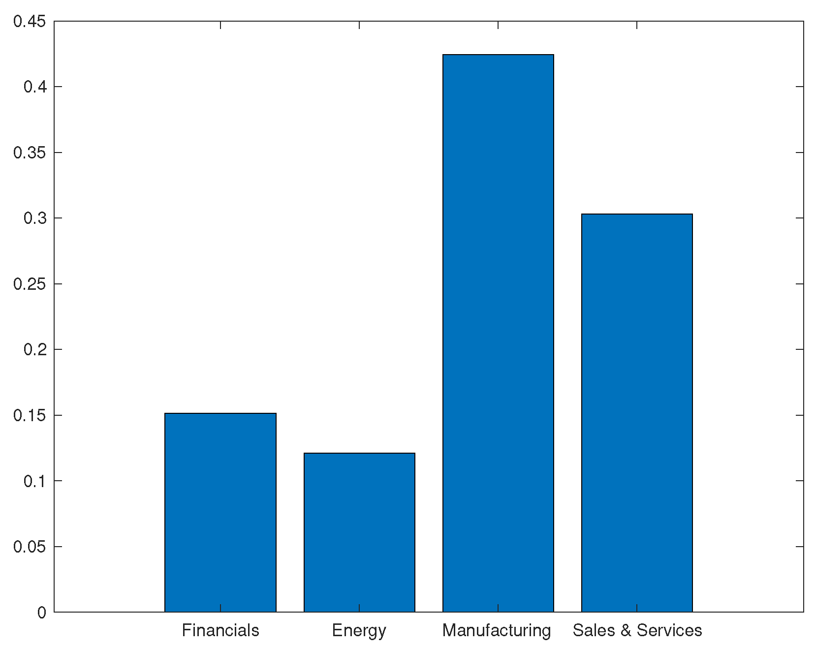
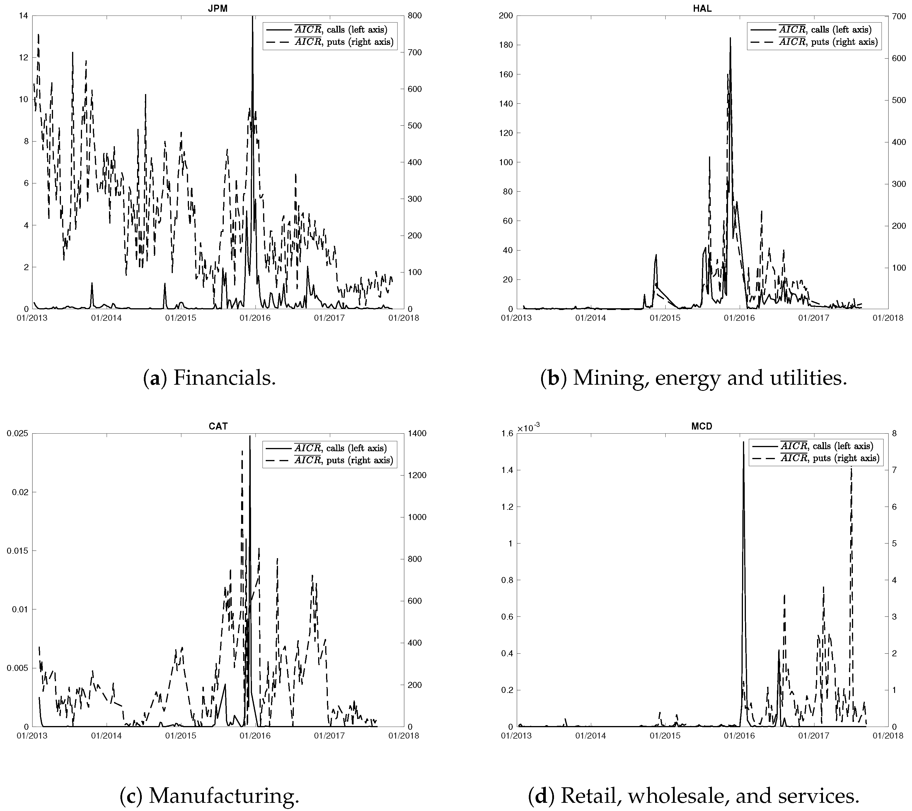
5.2. Sub-Samples Analysis Based on Sectors

In order to investigate further the link between options and credit risk, the same regressions in (13) are re-estimated over the four sub-samples based on industry (therefore, the industry-fixed effect is removed, whilst the year-fixed effect is kept). Based on the findings in Carr and Wu (2017), a cross-sectional diversity should emerge. Only put options are taken into consideration as the impact of default risk on call options was shown to be insignificant. Results are reported in

Table 6. Estimation of regression (13) over the four sub-samples. (a): Estimates of the year-fixed effect panel regression of market model-implied leverage $LEV$ onto average $AICR$ calculated over put options and CDSs of Financials. Number of observations: 1851 F-stat = 221.76 (p-value = 0.000). (b): Estimates of the year-fixed effect panel regression of market model-implied leverage $LEV$ onto average $AICR$ calculated over put options and CDSs of Mining, Energy and Utilities. Number of observations: 1900. F-stat = 63.75 (p-value = 0.000). (c): Estimates of the year-fixed effect panel regression of market model-implied leverage $LEV$ onto average $AICR$ calculated over put options and CDSs of Manufacturing. Number of observations: 6489. F-stat = 19.36 (p-value = 0.000). (d): Estimates of the year-fixed effect panel regression of market model-implied leverage $LEV$ onto average $AICR$ calculated over put options and CDSs of Retail, Wholesale and Services. Number of observations: 4655. F-stat = 120.89 (p-value = 0.000). A sandwich estimator for panel data is used to obtain robust standard errors. Significance levels: 10% (*), 5% (**), 1% (***).

(a): Financials
Regressand				Adj-$R^2$:	0.5205
${\overline{AICR}}_{-1}^{\prime }$
Regressors	Coefficient	Robust Standard Error	t-stat	p-value
$LEV$	0.0255	0.0008	32.20	0.000	***
${\alpha }_{-1}$	−0.0092	0.0012	−7.50	0.000	***
Year−FE	✓
(b): Mining, Energy and Utilities
Regressand				Adj-$R^2$:	0.3916
${\overline{AICR}}_{-1}^{\prime }$
Regressors	Coefficient	Robust Standard Error	t-stat	p-value
$LEV$	0.0200	0.0013	15.72	0.000	***
${\alpha }_{-1}$	−0.0013	0.0005	−2.69	0.007	***
Year−FE	✓
(c): Manufacturing
Regressand				Adj-$R^2$:	0.3541
${\overline{AICR}}_{-1}^{\prime }$
Regressors	Coefficient	Robust Standard Error	t-stat	p-value
$LEV$	0.0249	0.0031	8.08	0.000	***
${\alpha }_{-1}$	−0.0040	0.0006	−6.87	0.000	***
Year−FE	✓
(d): Retail, Wholesale and Services
Regressand				Adj-$R^2$:	0.1081
${\overline{AICR}}_{-1}^{\prime }$
Regressors	Coefficient	Robust Standard Error	t-stat	p-value
$LEV$	0.0009	0.0001	14.38	0.000	***
${\alpha }_{-1}$	0.0001	0.00002	4.91	0.000	***
Year−FE	✓

.

Financial firms tend to actively manage their capital structures according to changes in market conditions and to satisfy regulatory requirements. The results indeed capture the impact of credit risk to be driven by financial leverage (highest adjusted $R^2$ and significance). Similarly, put prices of utility and energy companies seem to be influenced by credit risk as well. Operating in regulated businesses and being strongly influenced by systemic factors as the state of the economy, perhaps the regression fit could be enhanced accounting for macroeconomic factors.

As manufacturing companies usually invest in long-term assets, they tend to have the same debt for a long period of time, without actively rebalancing their capital structure. Therefore, their financial leverage varies passively with the stock price fluctuations. Also, in addition to having a relatively small average ${\overline{AICR}}_{-1}^{\prime }$ (see

Table 7. Sub-sample averages for leverage and $\overline{AICR}$ obtained from put options and CDSs.

	Financials	Energy and Utilities	Manufacturing	Sales and Services
$\overline{LEV}$	1.3436	0.4478	0.2237	0.2286
${\overline{\overline{AICR}}}_{-1}^{\prime }$	0.0265	0.0072	0.0008	0.0033

), they also have the smallest mean leverage across the categories. This could explain the lower power of leverage in driving the company credit risk (which is however small).

The same conclusion applies to companies operating in sales and services, despite to a much weaker extent: given an average leverage comparable to manufacturing companies, they also show relatively small ${\overline{AICR}}_{-1}^{\prime }$. The regression adjusted $R^2$ is almost a fifth of that obtained from financial companies.

Unreported results available upon request show that these findings across the four sub-samples still hold after having accounted for a firm-fixed effect.

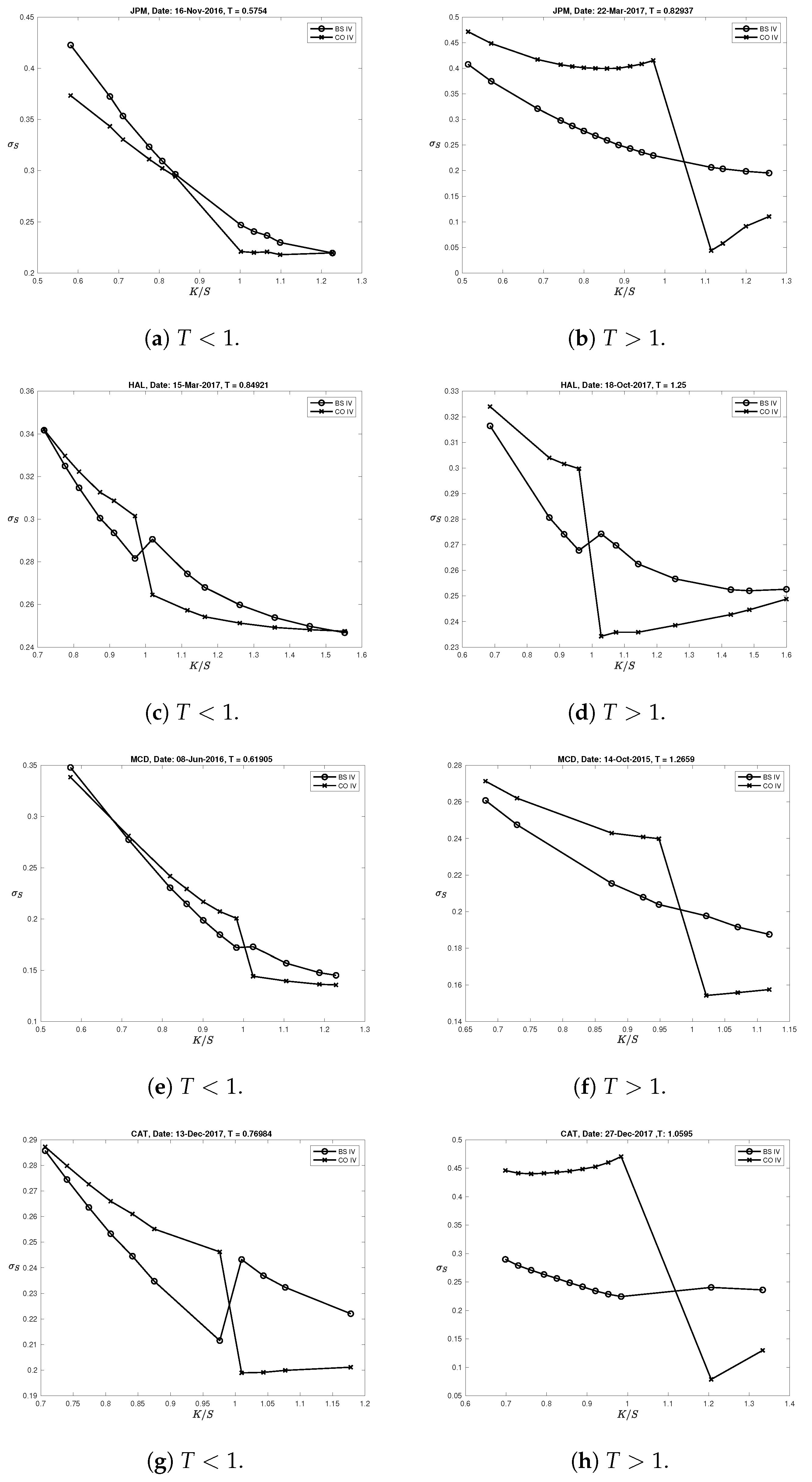
5.3. Explaining the Skew

Many attempts have been made in the literature in order to explain the shapes of the implied volatilities obtained from options. It is well-known that inverting the Black–Scholes formula to determine the value of the volatility which matches the observed price produces the so called volatility smile or smirk, instead of a flat line as predicted by the Black–Scholes model. Furthermore, it has been extensively documented that equity volatilities display more often a smirk rather than a smile: equity volatility is a decreasing and convex function of the moneyness of the option. The negative slope of the implied volatility function is referred to as negative skew.

The first works attempting to give a explanation for the observed skew are Black (1976) and Christie (1982). Both attribute the negative slope to the possibility of the underlying to default, the so-called leverage effect: if the underlying of the option can default, the left tail of its distribution should be more sensitive to credit-related events which notoriously make the value of the firm’s equity significantly drop. This increased probability of the underlying falling due to default would be then reflected in the pricing of options. Also, as put options protects the buyer against price falling, they should price both market- and credit-related events. As shown in Section 5.1, put options indeed price credit risk (and doubtlessly price market risk). However, some more recent works shed light on the drivers of the volatility skew.

Carr and Wu (2017) show that the leverage effect can be generated by other sources than leverage. As a matter of fact, the skew is also displayed by other assets, such as commodities or indexes, which cannot default. In their work, they individuate three possible channels influencing volatility: (1) return volatility increases with financial leverage; (2) positive shocks to systematic risk generate a negative correlation between the market’s return and its volatility, regardless of the magnitude of financial leverage; (3) large negative market disruptions show self-exciting behaviours.

Their estimations show that the volatility feedback effect (2) reveals itself mainly in the variations of short-term options, the self-exciting behaviour (3) affects both short-term and long-term option variations, and the financial leverage variation (1) has its largest impact on long-dated options. Finally, when the model of Carr and Wu (2017) is applied to individual companies, the three economic channels show up differently and to different degrees according to the company’s specific business and capital structure. Therefore, their work constitutes a valuable ruler in order to asses the compound option model predictions and results.

From a different perspective, the shape of the volatility smile/smirk provides an insight on how the Black–Scholes model (mis)prices risk under the presence of both market and credit risk, and how the estimation of the implied volatility is affected by them. Figure 4 suggests that the Black–Scholes implied volatility is an average of the implied volatility estimated with a compound option model (which, instead, allows us to account for the relative impact of credit and market risk separately).

Evidently, the Black–Scholes averages across the surface the impact of credit risk. Analytically, the probabilities involved in the calculation of the option price à la Black–Scholes are of the type

$$\mathbb{Q}\left(\xi S_T>\xi K\right)$$

whilst those of the compound option model are of the type

$$\mathbb{Q}\left(\xi S_T>\xi K|\tau >t_i\right).$$

By the law of total probability

$$\mathbb{Q}\left(\xi S_T>\xi K\right)={\mathbb{E}}^{\mathbb{Q}}\left[\mathbb{Q}\left(\xi S_T>\xi K|\tau >t_i\right)\right],$$

thus showing that the probabilities involved in the Black–Scholes model are an average of the probability of the option expiring in-the-money conditional upon the firm surviving at the reimbursement dates. Therefore, the volatility smirk produced by Black–Scholes should lie within the implied volatilities produced by the model. Figure 4 confirms this intuition.

Inspecting Figure 4, the averaging impacts mostly long-maturity options as the underlying probability of defaulting increases with the time horizon. Interestingly, for financial companies, despite displaying a negative slope for both short and long-term maturity options, the skew is more likely to be associated with the leverage effect for long-maturity options only (panel (b)). As a matter of fact, the compound option implied volatilities of the short-term maturity options of financial companies (panel (a)), despite being highly levered, replicate almost perfectly the Black–Scholes implied volatility which does not accommodate for default risk explicitly.

More generally, the closer the two volatility smirks are, the lower the probability of default and therefore the impact of credit risk (i.e., leverage effect) on the pricing of the option. Also, a lower the probability of default should correspond to a flatter smirk.

Notice also that, if ${\sum }_i{F}_i\downarrow 0$, the compound option model coincides with Black and Scholes (1973). Therefore, the larger the firm’s financial leverage the farther the Black–Scholes implied volatilities surface should be with respect to those estimated via the compound option model. However, if the two models reproduce very similar volatility skews even when the company is highly levered (e.g., financials), it can be argued that ‘apparent’ leverage effect is not driven by leverage and, therefore, financial leverage is not a good proxy for default risk, at least in the short-term. This is exactly what Carr and Wu (2017) document.14

Moving to the explanation of the observed skew, which is the negative slope displayed by the graph of the implied volatility plotted against moneyness, we adopt the definition provided by Carr and Wu (2017), that is

$$\mathrm{Skew}=\frac{25\Delta \mathrm{Put}{\sigma }_{IV}-25\Delta \mathrm{Call}{\sigma }_{IV}}{50\Delta \mathrm{Put}{\sigma }_{IV}},$$

(15)

where $x\Delta$Put${\sigma }_{IV}$ is the implied volatility of the put option whose delta is $-x\%$, and $y\Delta$Call${\sigma }_{IV}$ is the implied volatility of the call with delta equal to $y\%$. The proposed measure of skewness is more positive when the risk-neutral return distribution is more negatively skewed.

In order to investigate to what extent the displayed skew is driven by leverage, the following panel regression are carried out

$$\Delta {\mathrm{Skew}}_{j,t,T}={\alpha }_T+{\varphi }_{j,T}+{\theta }_{y,T}+\beta {\overline{AICR}}_{j,t-1,-1,T}+{\epsilon }_{j,t,y,T},$$

(16)

where ${\overline{AICR}}_{j,t-1,T,-1}$ is the average $AICR$ of put options having time to maturity equal to T observed in the previous week. Rather than using industry-fixed effect, a firm-fixed effect (${\varphi }_j$) is estimated as, ultimately, we want to show the ability of this measure to forecast future changes in the skew observed at the company level. If the skew is caused by the leverage effect, a positive and statistically significant effect should be observed.

The variable $\Delta \mathrm{Skew}$ is calculated based on (15). Call options are excluded, given the results in Section 5.1. Also, $\Delta \mathrm{Skew}$ is used rather than the contemporaneous level as the time-series component of the latter is non-stationary for some companies (see Figure 5).

In particular, based on the previous findings, two sets of regression are estimated. As for every day t, multiple maturities are observed, the skew of the shortest (${min}_T:T<1$ year) and longest (${max}_T:T>1$ year) maturity options is used in two separate sets of regressions. Based on the different behaviour of the model for short and long term maturity options, the skew should be driven by credit risk (here proxied as the $\overline{AICR}$ of out-of-the-money put options) mostly for $T>1$ rather than for $T<1$.

The estimates are presented in

Table 8. Estimation of regression (16). (a): Predictive regression for short-term skew based on the average $ICR$ calculated over short-term put options and CDSs. Number of observations: 7746. F-stat = 8.89 (p-value = 0.000). (b): Predictive regression for long-term skew based on the average $ICR$ calculated over long-term put options and CDSs. Number of observations: 6817. F-stat = 13.59 (p-value = 0.000). A sandwich estimator for panel data is used to obtain robust standard errors. Significance levels: 10% (*), 5% (**), 1% (***).

(a): Predictive regression for short-term skew.
Regressand				$R^2$ (between):	0.0036
$\Delta {\mathrm{Skew}}_{T<1}$				$R^2$ (within):	0.0004
Regressors	Coefficient	Robust Standard Error	t-stat	p-value
${\overline{AICR}}_{-1,T<1}^{\prime }$	−0.4308	0.9730	−0.44	0.659
${\alpha }_{T<1}$	−0.0035	0.0009	−3.81	0.000	***
firm−FE	✓
year−FE	✓
(b): Predictive regression for long-term skew.
Regressand				$R^2$ (between):	0.3096
$\Delta {\mathrm{Skew}}_{T>1}$				$R^2$ (within):	0.0004
Regressors	Coefficient	Robust Standard Error	t-stat	p-value
${\overline{AICR}}_{-1,T>1}^{\prime }$	0.3360	0.0956	3.51	0.001	***
${\alpha }_{T>1}$	−0.0108	0.0017	−6.36	0.000	***
firm−FE	✓
year−FE	✓

. Consistently with economic intuition and the empirical evidence in Carr and Wu (2011, 2017), only the changes in the skew of long-maturity options are driven by the credit risk of the company. Also, the average $AICR$ of put options, is able, to some extent, to predict the future changes in the skew for those options. The same variable is not able to explain the movements of the skew for options with shorter maturities. Therefore, the high significance of the average $AICR$ obtained from put options, as well as the correct sign of its loading, points towards a connections between the future changes of the negative skew and the today’s credit risk of the company. However, the low fit is likely to be attributed either to the presence of other factors driving the skew or to the highly non-linear link between the movements of the skew and the impact of credit risk (or both).

The fact that the $R^2$-between is much larger than the $R^2$-within (which is virtually zero) shows a greater ability of (16) to describe the cross-sectional variation rather than the time-series component of the changes in the skew.

6. Conclusions

To the best of our knowledge, this is the first work which explores and rigorously assesses the impact of credit risk on equity calls and puts using a large sample of options (both in the cross-section and the time-series dimension).

In this paper, we investigate the effect of credit-related events on the pricing of equity options. Given a firm which has issued $n\ge 1$ defaultable coupon-bearing bonds, we generalise the results in Merton (1974) and Geske (1977), and price the firm’s equity as an n–fold compound option call option on the asset value struck at the face values of the bonds outstanding. Further, we extend the pricing formula in Geske (1979) and show that European vanilla options on the firm’s equity are $(n+1)$-fold compound options written on the value of the firm’s assets.

Given the functional form of the pricing equations of the compound option model, a new measure of impact of credit risk based on option prices is constructed, thus allowing us to rank the latter based on how much they are exposed to credit-related events. Consistent with the economic intuition and the results in Carr and Wu (2011) (who, instead, opt for a reduced-form approach to model default), call and put option prices are influenced very differently by the possibility of the company defaulting. More specifically, as expected, call options do not price credit risk as much as put options do. In fact, during normal times, the proposed measure $AICR$ is consistently larger for put options compared to calls. However, we also showed that when the market factors the fear of an upcoming recession (such as at the end of 2015) into option prices, both $AICR$ measures on calls and puts spiked. This suggests a timely reactiveness and economic soundness of the proposed measure.

Furthermore, we show that the pricing information in terms of default events carried by CDSs and put options via their respective default probabilities are consistent with one another. This may suggest a high degree of integration between the two markets, thus ruling out possible arbitrage opportunities (i.e., if, say, the deep-out-the money 1-year put is mispriced with respect to the CDS with identical tenor written on the same entity, one could sell the more expensive and buy the cheapest to achieve an arbitrage profit in case of default).

We finally attempt at predicting the future changes in the negative skew displayed by equity options, and we show that the novel measure of credit risk constructed on put prices is able to forecast the cross-sectional differences in the changes of the skew for long-maturity equity options. Further work is however required to capture these movements more precisely. Factors based on the channels described in Carr and Wu (2017) could be constructed in order to improve the fit of the proposed regressions.

The implications of this study are multifaceted. Given the importance of default risk for those assets which are more sensitive to events occurring in the left tail of equity distribution (e.g., put options), risk-management implications for those instruments are relevant, especially when the underlying is the equity of either highly levered or financially distressed companies.

As a matter of fact, hedge funds often build highly levered positions in corporate bonds while hedging away interest rate risk by going short on treasuries. Thus, their hedged portfolios are mostly sensitive to changes in credit spreads rather than changes in the level, slope and curvature of the yield curve. Give a the possibility of large negative jumps in firm assets, then the appropriate hedging tool for corporate debt is not likely to be the firm’s stock, but rather deep out-of-the-money puts written on the equity of the same entity. In turn, the writer of these options will need to hedge its short position.

It is trivial to show that the Delta-hedge under the Black–Scholes model, which ignores credit risk, is different than the hedge prescribed by a compound option model. In fact, ignoring dividends for simplicity, the Delta-hedges under the Black–Scholes ($BS$) and a compound option ($CO$) model differ as such:

$$\frac{\partial P_{\xi }^{CO}}{\partial S}=\frac{\partial P_{\xi }^{CO}/\partial V}{\partial S/\partial V}\ne \xi \Phi \left(\xi d_1\right)=\frac{\partial P_{\xi }^{BS}}{\partial S}.$$

This inconsistency between the Black–Scholes and the compound option Greeks applies to any other hedging strategy based on the option sensitivities as long as credit risk is not accounted for, and these discrepancies become more and more severe for increasingly levered firms. A more in-depth analysis of this imperfect hedging when default risk is not taken into account is though left for future research.

As every empirical analysis, our work is also subject to some limitations. In particular, a plethora of models of default, both reduced-form and structural, have been proposed in the literature and could be used to measure default probabilities. Focusing on the structural models of default which the compound option model belongs to, we recognize that other factors such as the inclusion of taxes (Leland 1994; Leland and Toft 1996), strategic default (Anderson and Sundaresan 1996; Mella-Barral and Perraudin 1997), a default barrier (Black and Cox 1976), or other frictions, might be relevant for a more accurate modelling of default dynamics. The reason for working with a compound option model is due to the fact that it easily allows us to separate short- versus long-term default, being also the corresponding liabilities directly available from accounting data. It furthermore allows us to define the proposed measure of credit risk on equity option based on the information content of default events, and thus connecting it to the risk-neutral entropy of default probabilities.

References

1. Anderson, Ronald, and Suresh Sundaresan. 1996. Design and valuation of debt contracts. Review of Financial Studies 9: 37–68. [Google Scholar] [CrossRef]
2. Andreou, Panayiotis C. 2015. Effects of market default risk on index option risk-neutral moments. Quantitative Finance 15: 2021–40. [Google Scholar] [CrossRef]
3. Black, Fischer. 1976. Studies of stock price volatility changes. In Proceedings of the 1976 Meeting of the Business and Economic Statistics Section. Washington, DC: American Statistical Association, pp. 177–81. [Google Scholar]
4. Black, Fischer, and John C. Cox. 1976. Valuing corporate securities: Some effects of bond indenture provisions. Journal of Finance 31: 351–67. [Google Scholar] [CrossRef]
5. Black, Fischer, and Myron Scholes. 1973. The pricing of options and corporate liabilities. Journal of Political Economy 81: 637–54. [Google Scholar] [CrossRef]
6. Blanco, Roberto, Simon Brennan, and Ian. W. Marsh. 2005. An empirical analysis of the dynamic relation between investment-grade bonds and credit default swaps. Journal of Finance 60: 2255–81. [Google Scholar] [CrossRef]
7. Brigo, Damiano, and Fabio Mercurio. 2006. Interest Rate Models: Theory and Practice. Berlin and Heidelberg: Springer Finance. [Google Scholar]
8. Burkovska, Olena, Maximilian Gass, Kathrin Glau, Mirco Mahlstedt, Wim Schoutens, and Barbara Wohlmuth. 2018. Calibration to american options: Numerical investigation of the de-americanization method. Quantitative Finance 18: 1091–113. [Google Scholar] [CrossRef] [PubMed]
9. Campbell, John. Y., and Glen. B. Taksler. 2003. Equity volatility and corporate bond yields. Journal of Finance 58: 2321–49. [Google Scholar] [CrossRef]
10. Cao, Charles, Fan Yu, and Zhaodong Zhong. 2010. The information content of option-implied volatility for credit default swap valuation. Journal of Financial Markets 13: 321–43. [Google Scholar] [CrossRef]
11. Carr, Peter, and Liuren Wu. 2007. Theory and evidence on the dynamic interactions between sovereign credit default swaps and currency options. Journal of Banking and Finance 31: 2383–403. [Google Scholar] [CrossRef]
12. Carr, Peter, and Liuren Wu. 2010. Stock options and credit default swaps: A joint framework for valuation and estimation. Journal of Financial Econometrics 8: 409–49. [Google Scholar] [CrossRef]
13. Carr, Peter, and Liuren Wu. 2011. A simple robust link between american puts and credit protection. Review of Financial Studies 24: 473–505. [Google Scholar] [CrossRef]
14. Carr, Peter, and Liuren Wu. 2017. Leverage effect, volatility feedback, and self-exciting market disruptions. Journal of Financial and Quantitative Analysis 52: 2119–56. [Google Scholar] [CrossRef]
15. Carr, Peter, and Vadim Linetsky. 2006. A jump to default extended CEV model: An application of Bessel processes. Finance and Stochastics 10: 303–30. [Google Scholar] [CrossRef]
16. Christie, Andrew A. 1982. The stochastic behavior of common stock variances: Value, leverage and interest rate effects. Journal of Financial Economics 10: 407–32. [Google Scholar] [CrossRef]
17. Collin-Dufresne, Pierre, Robert S. Goldstein, and Fan Yang. 2012. On the relative pricing of long-maturity index options and collateralized debt obligations. Journal of Finance 67: 1983–2014. [Google Scholar] [CrossRef]
18. Collin-Dufresne, Pierre, Robert S. Goldstein, and J. Spencer Martin. 2001. The determinants of credit spread changes. Journal of Finance 56: 2177–207. [Google Scholar] [CrossRef]
19. Cover, Thomas M., and Joy A. Thomas. 2006. Elements of Information Theory. Hoboken: Wiley-Blackwell. [Google Scholar]
20. Cremers, K. J. Martijn, Joost Driessen, and Pascal Meanhout. 2008a. Explaining the level of credit spreads: Option-implied jump risk premia in a firm value model. Review of Financial Studies 21: 2209–42. [Google Scholar] [CrossRef]
21. Cremers, K. J. Martijn, Joost Driessen, Pascal Meanhout, and David Weinbaum. 2008b. Individual stock-option prices and credit spreads. Journal of Banking and Finance 32: 2706–15. [Google Scholar] [CrossRef]
22. Culp, Christopher L., Yoshio Nozawa, and Pietro Veronesi. 2018. Option-based credit spreads. American Economic Review 108: 454–88. [Google Scholar] [CrossRef]
23. Duffie, Darrell, and Kenneth J. Singleton. 1999. Modeling term structures of defaultable bonds. Review of Financial Studies 12: 687–720. [Google Scholar] [CrossRef]
24. Elton, Edwin J., J. Gruber Martin, Deepak Agrawal, and Christopher Mann. 2001. Explaining the rate spread on corporate bonds. Journal of Finance 56: 247–77. [Google Scholar] [CrossRef]
25. Ericsson, Jan, Kris Jacobs, and Rodolfo Ovied. 2009. The determinants of credit default swap premia. Journal of Financial and Quantitative Analysis 44: 109–32. [Google Scholar] [CrossRef]
26. Geske, Robert 1977. The valuation of corporate liabilities as compound options. Journal of Financial and Quantitative Analysis 12: 541–52.
27. Geske, Robert. 1979. The valuation of compound options. Journal of Financial Economics 7: 63–81. [Google Scholar] [CrossRef]
28. Geske, Robert, Avanidhar Subrahmanyam, and Yi Zhou. 2016. Capital structure effects on the prices of equity call options. Journal of Financial Economics 36: 1639–52. [Google Scholar] [CrossRef]
29. Huang, Jing-Zhi, and Ming Huang. 2012. How much of the corporate-treasury yield spread is due to credit risk? Review of Asset Pricing Studies 2: 153–202. [Google Scholar] [CrossRef]
30. Hull, John, and Alan White. 1995. The impact of default risk on the prices of options and other derivative securities. Journal of Banking and Finance 9: 299–322. [Google Scholar] [CrossRef]
31. Hull, John C., Izzy Nelkenand, and Alan D. White. 2004. Merton’s model, credit risk and volatility skews. Journal of Credit Risk 1: 3–28. [Google Scholar] [CrossRef]
32. Jarrow, Robert A., and Stuart M. Turnbull. 1995. Pricing derivatives on financial securities subject to credit risk. Journal of Finance 50: 53–85. [Google Scholar] [CrossRef]
33. Johnson, Herb, and René Stulz. 1987. The pricing of options with default risk. Journal of Finance 42: 267–80. [Google Scholar] [CrossRef]
34. Leland, Hayne, and Klaus Bjerre Toft. 1996. Optimal capital structure, endogenous bankruptcy, and theterm structure of credit spreads. Journal of Finance 51: 987–1019. [Google Scholar] [CrossRef]
35. Leland, Hayne E. 1994. Corporate debt value, bond covenants, and optimal capital structure. Journal of Finance 49: 1213–52. [Google Scholar] [CrossRef]
36. Maglione, Federico. 2022. Credit spreads, leverage and volatility: A cointegration approach. Computation 10: 155. [Google Scholar] [CrossRef]
37. Mella-Barral, Pierre, and William Perraudin. 1997. Strategic debt service. Journal of Finance 52: 531–66. [Google Scholar] [CrossRef]
38. Mendoza-Arriga, Rafael, Peter Carr, and Vadim Linetsky. 2010. Time-changed Markov processes in unified credit-equity modeling. Mathematical Finance 20: 527–69. [Google Scholar] [CrossRef]
39. Merton, Robert C. 1974. On the pricing of corporate debt: The risk structure of interest rates. Journal of Finance 29: 449–70. [Google Scholar]
40. Merton, Robert C. 1977. On the pricing of contingent claims and the Modigliani-Miller theorem. Journal of Financial Economics 5: 241–9. [Google Scholar] [CrossRef]
41. Strebulaev, Ilya A., and Toni M. Whited. 2012. Dynamic Models and Structural Estimation in Corporate Finance. Boston: Now Publishers Inc. [Google Scholar]
42. Toft, Klaus Bjerre, and Brian Prucyk. 1997. Options on leveraged equity: Theory and empirical tests. Journal of Finance 53: 1151–80. [Google Scholar] [CrossRef]
43. Vasquez, Aurelio, and Xiao Xiao. 2023. Default risk and option returns. Management Science. [Google Scholar] [CrossRef]
Figure 1. Industry/sector composition of the whole sample: Financial companies (15%); Mining, Energy and Utilities companies (12%); Manufacturing (42%); Retail, Wholesales and Services (30%).
Risks 11 00183 g001
Figure 2. Empirical distributions of moneyness ( K / S ) and maturity ( T ) of option data. Panel (a) shows that most of the valid call option observations have moneyness in ( 1 , 1.8 ) , whilst for put options, displayed in panel (b), the moneyness is in ( 0.6 , 1 ) . The distribution of put options is less peaked than the one of calls. Panels (c,d) takes into account the maturities of the options which range from 0.5 to 2.4 years form both call and put quotes, being the distributions very similar.
Risks 11 00183 g002
Figure 3. Comparison of daily average A I C R calculated over call and put options for four companies representing the four selected industries/sectors. As expected, A I C R ¯ calculated using call (solid lines) options is much smaller than those obtained from put (dashed lines) options. A I C R ¯ s are expressed in basis points. Sub-figures (ad) display the A I C R ¯ measure for companies operating in different sectors.
Risks 11 00183 g003
Figure 4. Volatility skews for different option maturities. The lines marked with circles are the implied volatility estimates produced by the Black–Scholes model, whilst those marked with crosses are the estimates produced by the compound option model. It is evident that the Black–Scholes estimates of the implied volatility lie within the estimates produced by the model, thus suggesting the aforementioned averaging effect. This effect is more pronounced for long-term maturity options (panels (b,d,f,h)) than for options with shorter maturities (panels (a,c,e,g)), as the distance between the two lines is larger for T > 1 .
Risks 11 00183 g004
Figure 5. Time-series of skew extracted from short-term maturity options ( T < 1 , panel (a)) and from long-term maturity options ( T > 1 , panel (b)) for AAPL. Both panels show that the time series of the levels of Skew (dotted-dashed line) is non-stationary whilst the increments (solid line) are stationary.
Risks 11 00183 g005