
Dependence Modelling of Lifetimes in Egyptian Families


Abstract
1. Introduction
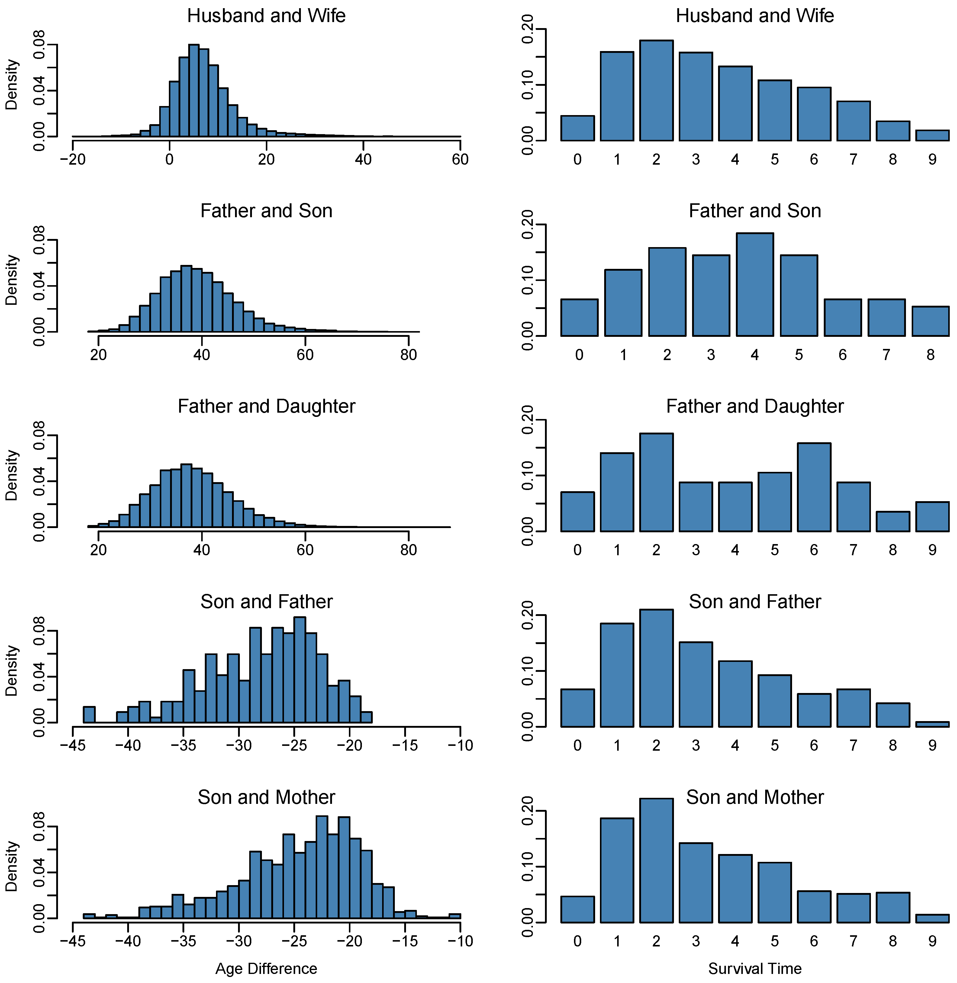
2. Data Set
3. Model Description
4. Metropolis–Hastings MCMC
- Initialise, i.e., draw from the prior distribution.
- For
- -
- Sample the proposal for from .
- -
- Computewhere A defines the acceptance probability.
- -
- Draw . If , accept the proposal, fixing . Else, fix .
5. Inference Functions for Margins
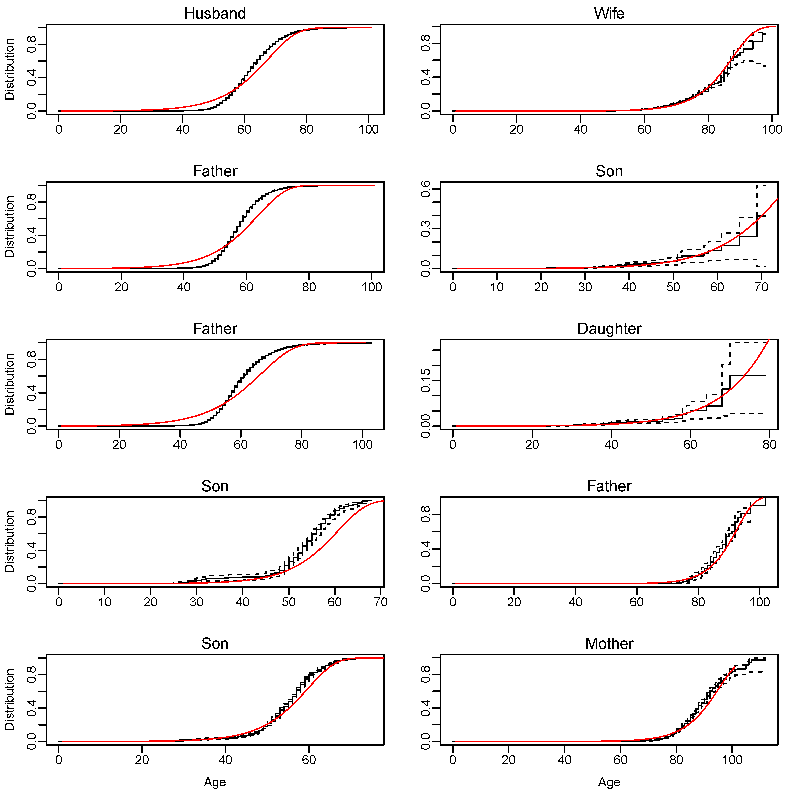
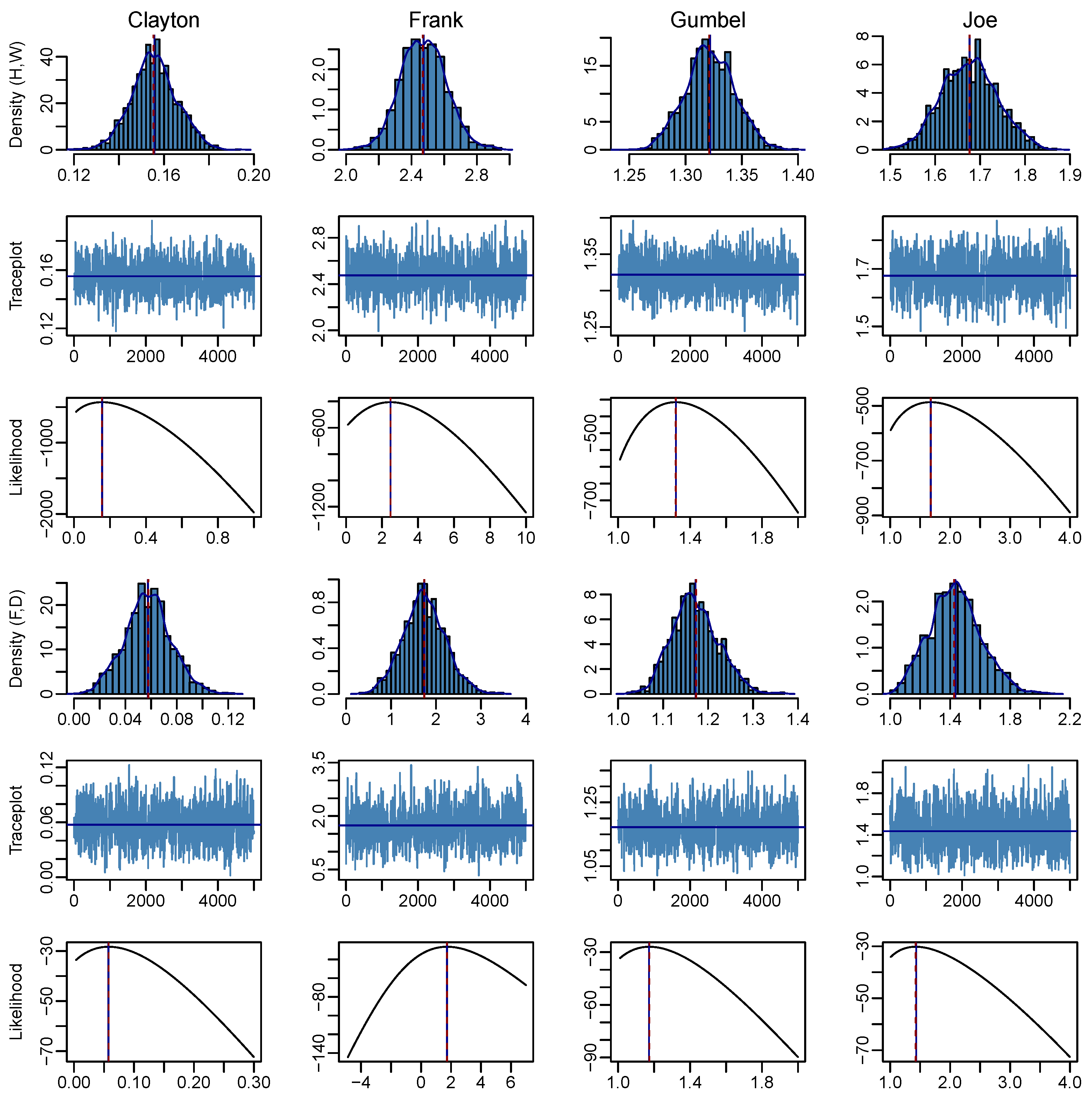
6. Results

| MCMC | MLE | |||||||
|---|---|---|---|---|---|---|---|---|
| Estimate | Acceptance | SD | IAT | SE | Estimate | SE | ||
| (H,W) | 66.79 | 0.2573 | 0.06765 | 9.303 | 0.002918 | 66.80 | 0.06923 | |
| 9.076 | 0.2573 | 0.04583 | 6.609 | 0.001666 | 9.078 | 0.04436 | ||
| 86.65 | 0.2486 | 0.3638 | 25.77 | 0.02612 | 86.66 | 0.3671 | ||
| 6.958 | 0.2486 | 0.1342 | 18.42 | 0.008143 | 6.955 | 0.1342 | ||
| (F,S) | 62.61 | 0.2769 | 0.1016 | 9.590 | 0.004448 | 62.61 | 0.1004 | |
| 8.973 | 0.2769 | 0.06157 | 7.239 | 0.002342 | 8.973 | 0.05980 | ||
| 75.38 | 0.2438 | 2.942 | 93.84 | 0.4030 | 74.48 | 2.583 | ||
| 9.244 | 0.2438 | 0.6400 | 78.79 | 0.08033 | 9.053 | 0.5774 | ||
| (F,D) | 65.73 | 0.2529 | 0.1091 | 10.36 | 0.004967 | 65.73 | 0.1158 | |
| 10.65 | 0.2529 | 0.07023 | 7.125 | 0.002651 | 10.64 | 0.07252 | ||
| 89.91 | 0.2348 | 3.649 | 118.9 | 0.5628 | 89.29 | 3.598 | ||
| 10.15 | 0.2348 | 0.7810 | 99.46 | 0.1101 | 10.03 | 0.7776 | ||
| (S,F) | 59.69 | 0.2478 | 0.4648 | 11.26 | 0.02206 | 56.70 | 0.4417 | |
| 6.263 | 0.2478 | 0.3441 | 9.471 | 0.01498 | 6.199 | 0.3225 | ||
| 91.73 | 0.2360 | 0.5434 | 8.767 | 0.02275 | 91.70 | 0.5100 | ||
| 5.636 | 0.2360 | 0.3838 | 7.649 | 0.01501 | 5.554 | 0.3708 | ||
| (S,M) | 58.67 | 0.2601 | 0.2184 | 10.94 | 0.01022 | 58.67 | 0.2144 | |
| 6.640 | 0.2601 | 0.1482 | 8.864 | 0.006238 | 6.621 | 0.1488 | ||
| 94.23 | 0.2488 | 0.3679 | 9.668 | 0.01617 | 94.20 | 0.3578 | ||
| 7.289 | 0.2488 | 0.2385 | 7.572 | 0.009281 | 7.248 | 0.2323 | ||
6.1. Goodness-of-Fit
- Let B be the number of bootstrap samples. For
- -
- Simulate the paired remaining lifetimes , from the estimated copula , with Gompertz marginals distributed as in Table 5.
- -
- Fix and , , where 9 is the length of the observation period. If the censoring point is random, simulate , from its observed distribution.
- -
- Determine the b-th bootstrap observations from the data simulated in the preceding steps.
- -
- Estimate the marginal parameters and the copula dependence parameter of the bootstrap sample via the IFM procedure described in Section 5.
- -
- Compute the Cramér–von Mises statistic of the bootstrap sample using (A2).
7. Conclusions
Author Contributions
Funding
Institutional Review Board Statement
Informed Consent Statement
Data Availability Statement
Acknowledgments
Conflicts of Interest
Appendix A
| Copula | Generator | Domain | |
|---|---|---|---|
| Clayton | |||
| Frank | |||
| Gumbel | |||
| Joe |
| Kendall’s Tau | |
|---|---|
| Clayton | |
| Frank | |
| Gumbel | |
| Joe |
Appendix B
References
- Almeida, Carlos, and Claudia Czado. 2012. Efficient Bayesian inference for stochastic time-varying copula models. Computational Statistics & Data Analysis 56: 1511–27. [Google Scholar]
- Antonio, Katrien, Anastasios Bardoutsos, and Wilbert Ouburg. 2015. Bayesian Poisson log-bilinear models for mortality projections with multiple populations. European Actuarial Journal 5: 245–81. [Google Scholar] [CrossRef]
- Arias, Luis A. Souto, and Pasquale Cirillo. 2021. Joint and survivor annuity valuation with a bivariate reinforced urn process. Insurance: Mathematics and Economics 99: 174–89. [Google Scholar]
- Arjas, Elja, and Dario Gasbarra. 1996. Bayesian inference of survival probabilities, under stochastic ordering constraints. Journal of the American Statistical Association 91: 1101–9. [Google Scholar] [CrossRef]
- Ausin, M. Concepcion, and Hedibert F. Lopes. 2010. Time-varying joint distribution through copulas. Computational Statistics & Data Analysis 54: 2383–99. [Google Scholar]
- Biffis, Enrico. 2005. Affine processes for dynamic mortality and actuarial valuations. Insurance: Mathematics and Economics 37: 443–68. [Google Scholar] [CrossRef]
- Booth, Heather, and Leonie Tickle. 2008. Mortality modelling and forecasting: A review of methods. Annals of Actuarial Science 3: 3–43. [Google Scholar] [CrossRef]
- Brechmann, Eike C., Katharina Hendrich, and Claudia Czado. 2013. Conditional copula simulation for systemic risk stress testing. Insurance: Mathematics and Economics 53: 722–32. [Google Scholar] [CrossRef]
- Cabrignac, Olivier, Arthur Charpentier, and Ewen Gallic. 2020. Modeling joint lives within families. arXiv arXiv:2006.08446. [Google Scholar]
- Cairns, Andrew J. G., David Blake, and Kevin Dowd. 2006. A two-factor model for stochastic mortality with parameter uncertainty: Theory and calibration. Journal of Risk and Insurance 73: 687–718. [Google Scholar] [CrossRef]
- Cairns, Andrew J. G., David Blake, Kevin Dowd, Guy D. Coughlan, and Marwa Khalaf-Allah. 2011. Bayesian stochastic mortality modelling for two populations. ASTIN Bulletin: The Journal of the IAA 41: 29–59. [Google Scholar]
- Cairns, Andrew J. G., David Blake, Kevin Dowd, Guy D. Coughlan, David Epstein, Alen Ong, and Igor Balevich. 2009. A quantitative comparison of stochastic mortality models using data from England and Wales and the United States. North American Actuarial Journal 13: 1–35. [Google Scholar] [CrossRef]
- Carriere, Jacques F. 1992. Parametric models for life tables. Transactions of the Society of Actuaries 44: 77–99. [Google Scholar]
- Carriere, Jacques F. 1994. An investigation of the Gompertz law of mortality. Actuarial Research Clearing House 2: 161–77. [Google Scholar]
- Carriere, Jacques F. 2000. Bivariate survival models for coupled lives. Scandinavian Actuarial Journal 2000: 17–32. [Google Scholar] [CrossRef]
- Clayton, David G. 1978. A model for association in bivariate life tables and its application in epidemiological studies of familial tendency in chronic disease incidence. Biometrika 65: 141–51. [Google Scholar] [CrossRef]
- Czado, Claudia, Antoine Delwarde, and Michel Denuit. 2005. Bayesian Poisson log-bilinear mortality projections. Insurance: Mathematics and Economics 36: 260–84. [Google Scholar] [CrossRef]
- Dahl, Mikkel. 2004. Stochastic mortality in life insurance: Market reserves and mortality-linked insurance contracts. Insurance: Mathematics and Economics 35: 113–36. [Google Scholar] [CrossRef]
- da Rocha Neves, César, and Helio S. Migon. 2007. Bayesian graduation of mortality rates: An application to reserve evaluation. Insurance: Mathematics and Economics 40: 424–34. [Google Scholar] [CrossRef]
- da Silva Filho, Osvaldo Candido, Flavio Augusto Ziegelmann, and Michael J. Dueker. 2012. Modeling dependence dynamics through copulas with regime switching. Insurance: Mathematics and Economics 50: 346–56. [Google Scholar] [CrossRef]
- de Alba, Enrique. 2002. Bayesian estimation of outstanding claim reserves. North American Actuarial Journal 6: 1–20. [Google Scholar] [CrossRef]
- Denuit, Michel, and Anne Cornet. 1999. Multilife premium calculation with dependent future lifetimes. Journal of Actuarial Practice 7: 147–80. [Google Scholar]
- Denuit, Michel, Jan Dhaene, Celine Le Bailly de Tilleghem, and Stéphanie Teghem. 2001. Measuring the impact of dependence among insured lifelengths. Belgian Actuarial Bulletin 1: 18–39. [Google Scholar]
- Dufresne, François, Enkelejd Hashorva, Gildas Ratovomirija, and Youssouf Toukourou. 2018. On age difference in joint lifetime modelling with life insurance annuity applications. Annals of Actuarial Science 12: 350–71. [Google Scholar] [CrossRef]
- Egyptian Social Insurance and Pension Law 50. 1978. National Authority for Social Insurance (Egypt). Available online: https://nosi.gov.eg/ar/Pages/NOSIlibrary/NOSIlibrary.aspx?ncat=7 (accessed on 3 January 2023). (In Arabic)
- Egyptian Social Insurance and Pension Law 79. 1975. Section 18 (3). National Authority for Social Insurance (Egypt). Available online: https://nosi.gov.eg/ar/Pages/NOSIlibrary/NOSIlibrary.aspx?ncat=7 (accessed on 3 January 2023). (In Arabic)
- Egyptian Social Insurance and Pension Law 108. 1976. National Authority for Social Insurance (Egypt). Available online: https://nosi.gov.eg/ar/Pages/NOSIlibrary/NOSIlibrary.aspx?ncat=7 (accessed on 3 January 2023). (In Arabic)
- Egyptian Social Insurance and Pension Law 112. 1980. National Authority for Social Insurance (Egypt). Available online: https://nosi.gov.eg/ar/Pages/NOSIlibrary/NOSIlibrary.aspx?ncat=7 (accessed on 3 January 2023). (In Arabic)
- Egyptian Social Insurance and Pension Law 148. 2019. Sections 41, 98, 102, 105. National Authority for Social Insurance (Egypt). Available online: https://nosi.gov.eg/ar/Pages/NOSIlibrary/NOSIlibrary.aspx?ncat=7 (accessed on 3 January 2023). (In Arabic)
- El-Gohary, Awad, Ahmad Alshamrani, and Adel Naif Al-Otaibi. 2013. The generalized Gompertz distribution. Applied Mathematical Modelling 37: 13–24. [Google Scholar] [CrossRef]
- Frees, Edward W., Jacques Carriere, and Emiliano Valdez. 1996. Annuity valuation with dependent mortality. Journal of Risk and Insurance 63: 229–61. [Google Scholar] [CrossRef]
- Fung, Man Chung, Gareth W. Peters, and Pavel V. Shevchenko. 2019. Cohort effects in mortality modelling: A Bayesian state-space approach. Annals of Actuarial Science 13: 109–44. [Google Scholar] [CrossRef]
- Gavrilov, Leonid A., and Natalia S. Gavrilova. 2019. New trend in old-age mortality: Gompertzialization of mortality trajectory. Gerontology 65: 451–7. [Google Scholar] [CrossRef]
- Geerdens, Candida, Paul Janssen, and Noël Veraverbeke. 2016. Large sample properties of nonparametric copula estimators under bivariate censoring. Statistics 50: 1036–55. [Google Scholar] [CrossRef]
- Genest, Christian, and Nikolai Kolev. 2021. A law of uniform seniority for dependent lives. Scandinavian Actuarial Journal 2021: 726–43. [Google Scholar] [CrossRef]
- Genest, Christian, Bruno Rémillard, and David Beaudoin. 2009. Goodness-of-fit tests for copulas: A review and a power study. Insurance: Mathematics and Economics 44: 199–213. [Google Scholar] [CrossRef]
- Gobbi, Fabio, Nikolai Kolev, and Sabrina Mulinacci. 2019. Joint life insurance pricing using extended Marshall–Olkin models. ASTIN Bulletin: The Journal of the IAA 49: 409–32. [Google Scholar] [CrossRef]
- Gompertz, Benjamin. 1825. On the nature of the function expressive of the law of human mortality, and on a new mode of determining the value of life contingencies. Philosophical Transactions of the Royal Society of London 115: 513–83. [Google Scholar]
- Gourieroux, Christian, and Yang Lu. 2015. Love and death: A freund model with frailty. Insurance: Mathematics and Economics 63: 191–203. [Google Scholar] [CrossRef]
- Gribkova, Svetlana, and Olivier Lopez. 2015. Non-parametric copula estimation under bivariate censoring. Scandinavian Journal of Statistics 42: 925–46. [Google Scholar] [CrossRef]
- Guo, Guang. 1993. Use of sibling data to estimate family mortality effects in Guatemala. Demography 30: 15–32. [Google Scholar] [CrossRef]
- Henshaw, Kira, Corina Constantinescu, and Olivier Menoukeu Pamen. 2020. Stochastic mortality modelling for dependent coupled lives. Risks 8: 17. [Google Scholar] [CrossRef]
- Hong, Liang, and Ryan Martin. 2017. A flexible Bayesian nonparametric model for predicting future insurance claims. North American Actuarial Journal 21: 228–41. [Google Scholar] [CrossRef]
- Hougaard, Philip. 1984. Life table methods for heterogeneous populations: Distributions describing the heterogeneity. Biometrika 71: 75–83. [Google Scholar] [CrossRef]
- Hougaard, Philip. 2000. Analysis of Multivariate Survival Data. New York: Springer. [Google Scholar]
- Hougaard, Philip, Bent Harvald, and Niels V. Holm. 1992. Measuring the similarities between the lifetimes of adult Danish twins born between 1881–1930. Journal of the American Statistical Association 87: 17–24. [Google Scholar]
- Huard, David, Guillaume Evin, and Anne-Catherine Favre. 2006. Bayesian copula selection. Computational Statistics & Data Analysis 51: 809–22. [Google Scholar]
- Iachine, Ivan A., Niels V. Holm, Jennifer R. Harris, Alexander Z. Begun, Maria K. Iachina, Markku Laitinen, Jaakko Kaprio, and Anatoli I. Yashin. 1998. How heritable is individual susceptibility to death? The results of an analysis of survival data on Danish, Swedish and Finnish twins. Twin Research and Human Genetics 1: 196–205. [Google Scholar] [CrossRef]
- Jevtić, Petar, and Thomas R. Hurd. 2017. The joint mortality of couples in continuous time. Insurance: Mathematics and Economics 75: 90–97. [Google Scholar] [CrossRef]
- Ji, Min, Mary Hardy, and Johnny Siu-Hang Li. 2011. Markovian approaches to joint-life mortality. North American Actuarial Journal 15: 357–76. [Google Scholar] [CrossRef]
- Joe, Harry, and James J. Xu. 1996. The Estimation Method of Inference Functions for Margins for Multivariate Models. Technical Report. Vancouver: University of British Columbia Library. [Google Scholar]
- Khalil, Dalia. 2006. Dynamic Pension Funding Models. Ph.D. thesis, Cass Business School, London, UK. [Google Scholar]
- Klein, John P. 1992. Semiparametric estimation of random effects using the Cox model based on the EM algorithm. Biometrics 48: 795–806. [Google Scholar] [CrossRef]
- Krämer, Nicole, Eike C. Brechmann, Daniel Silvestrini, and Claudia Czado. 2013. Total loss estimation using copula-based regression models. Insurance: Mathematics and Economics 53: 829–39. [Google Scholar] [CrossRef]
- Lee, Gee Y., and Peng Shi. 2019. A dependent frequency–severity approach to modeling longitudinal insurance claims. Insurance: Mathematics and Economics 87: 115–29. [Google Scholar] [CrossRef]
- Li, Hong, and Yang Lu. 2018. A Bayesian non-parametric model for small population mortality. Scandinavian Actuarial Journal 2018: 605–28. [Google Scholar] [CrossRef]
- Li, Hong, Ken Seng Tan, Shripad Tuljapurkar, and Wenjun Zhu. 2021. Gompertz law revisited: Forecasting mortality with a multi-factor exponential model. Insurance: Mathematics and Economics 99: 268–81. [Google Scholar] [CrossRef]
- Lichtenstein, Paul, Niels V. Holm, Pia K. Verkasalo, Anastasia Iliadou, Jaakko Kaprio, Markku Koskenvuo, Eero Pukkala, Axel Skytthe, and Kari Hemminki. 2000. Environmental and heritable factors in the causation of cancer—Analyses of cohorts of twins from Sweden, Denmark, and Finland. New England Journal of Medicine 343: 78–85. [Google Scholar] [CrossRef]
- Lin, Tzuling, Chou-Wen Wang, and Cary Chi-Liang Tsai. 2015. Age-specific copula-AR-GARCH mortality models. Insurance: Mathematics and Economics 61: 110–24. [Google Scholar] [CrossRef]
- Luciano, Elisa, and Elena Vigna. 2005. Non-Mean Reverting Affine Processes for Stochastic Mortality. International Centre for Economic Research Applied Mathematics Working Paper No. 4. Available online: https://ssrn.com/abstract=724706 (accessed on 3 January 2023).
- Luciano, Elisa, and Elena Vigna. 2008. Mortality risk via affine stochastic intensities: Calibration and empirical relevance. Belgian Actuarial Bulletin 8: 5–16. [Google Scholar]
- Luciano, Elisa, Jaap Spreeuw, and Elena Vigna. 2008. Modelling stochastic mortality for dependent lives. Insurance: Mathematics and Economics 43: 234–44. [Google Scholar] [CrossRef]
- Luciano, Elisa, Jaap Spreeuw, and Elena Vigna. 2016. Spouses’ dependence across generations and pricing impact on reversionary annuities. Risks 4: 16. [Google Scholar] [CrossRef]
- Lu, Yang. 2017. Broken-heart, common life, heterogeneity: Analyzing the spousal mortality dependence. ASTIN Bulletin: The Journal of the IAA 47: 837–74. [Google Scholar] [CrossRef]
- Maeder, Philippe. 1995. La construction des tables de mortalite du tarif collectif 1995 de l’upav. Insurance: Mathematics and Economics 3: 226. [Google Scholar]
- Makeham, William Matthew. 1860. On the law of mortality and the construction of annuity tables. Journal of the Institute of Actuaries 8: 301–10. [Google Scholar] [CrossRef]
- Makeham, William Matthew. 1867. On the law of mortality. Journal of the Institute of Actuaries 13: 325–58. [Google Scholar]
- Marshall, Albert W., and Ingram Olkin. 1967. A multivariate exponential distribution. Journal of the American Statistical Association 62: 30–44. [Google Scholar] [CrossRef]
- Nelsen, Roger B. 2006. An Introduction to Copulas. New York: Springer Science & Business Media. [Google Scholar]
- Nielsen, Gert G., Richard D. Gill, Per Kragh Andersen, and Thorkild I. A. Sørensen. 1992. A counting process approach to maximum likelihood estimation in frailty models. Scandinavian Journal of Statistics 19: 25–43. [Google Scholar]
- Norberg, Ragnar. 1988. Actuarial analysis of dependent lives. Bulletin of the Swiss Association of Actuaries 2: 243–54. [Google Scholar]
- Ntzoufras, Ioannis, and Petros Dellaportas. 2002. Bayesian modelling of outstanding liabilities incorporating claim count uncertainty. North American Actuarial Journal 6: 113–25. [Google Scholar] [CrossRef]
- Oakes, David. 1989. Bivariate survival models induced by frailties. Journal of the American Statistical Association 84: 487–93. [Google Scholar] [CrossRef]
- Parkes, Colin. M., Bernard Benjamin, and Roy G. Fitzgerald. 1969. Broken heart: A statistical study of increased mortality among widowers. British Medical Journal 1: 740–43. [Google Scholar] [CrossRef]
- Pinto, Jayme, and Nikolai Kolev. 2015. Extended Marshall–Olkin model and its dual version. In Marshall–Olkin Distributions-Advances in Theory and Applications. Cham: Springer, pp. 87–113. [Google Scholar]
- Rees, W. Dewi, and Sylvia Lutkins. 1967. Mortality of bereavement. British Medical Journal 4: 13–16. [Google Scholar] [CrossRef]
- Robert, Christian P., and George Casella. 1999. The Metropolis—Hastings algorithm. In Monte Carlo Statistical Methods. New York: Springer, pp. 231–83. [Google Scholar]
- Roberts, Gareth O., and Jeffrey S. Rosenthal. 2004. General state space Markov chains and MCMC algorithms. Probability Surveys 1: 20–71. [Google Scholar] [CrossRef]
- Roberts, Gareth O., Andrew Gelman, and Walter R. Gilks. 1997. Weak convergence and optimal scaling of random walk Metropolis algorithms. The Annals of Applied Probability 7: 110–20. [Google Scholar]
- Sanders, Lisanne, and Bertrand Melenberg. 2016. Estimating the joint survival probabilities of married individuals. Insurance: Mathematics and Economics 67: 88–106. [Google Scholar] [CrossRef]
- Sastry, Narayan. 1997. Family-level clustering of childhood mortality risk in Northeast Brazil. Population Studies 51: 245–61. [Google Scholar] [CrossRef]
- Satten, Glen A., and Somnath Datta. 2001. The Kaplan–Meier estimator as an inverse-probability-of-censoring weighted average. The American Statistician 55: 207–10. [Google Scholar] [CrossRef] [PubMed]
- Schrager, David F. 2006. Affine stochastic mortality. Insurance: Mathematics and Economics 38: 81–97. [Google Scholar] [CrossRef]
- Scollnik, David P. M. 2001. Actuarial modeling with MCMC and BUGS. North American Actuarial Journal 5: 96–124. [Google Scholar] [CrossRef]
- Shemyakin, Arkady, and Heekyung Youn. 2001. Bayesian estimation of joint survival functions in life insurance. In Monographs of Official Statistics. Bayesian Methods with Applications to Science, Policy and Official Statistics. Luxembourg: European Communities. [Google Scholar]
- Shemyakin, Arkady, and Heekyung Youn. 2006. Copula models of joint last survivor analysis. Applied Stochastic Models in Business and Industry 22: 211–24. [Google Scholar] [CrossRef]
- Silva, Ralph dos Santos, and Hedibert Freitas Lopes. 2008. Copula, marginal distributions and model selection: A Bayesian note. Statistics and Computing 18: 313–20. [Google Scholar] [CrossRef]
- Sklar, M. 1959. Fonctions de repartition an dimensions et leurs marges. Publications de l’Institut de Statistique de l’Université de Paris 8: 229–31. [Google Scholar]
- Spreeuw, Jaap, and Iqbal Owadally. 2013. Investigating the broken-heart effect: A model for short-term dependence between the remaining lifetimes of joint lives. Annals of Actuarial Science 7: 236–57. [Google Scholar] [CrossRef]
- Spreeuw, Jaap, and Xu Wang. 2008. Modelling the short-term dependence between two remaining lifetimes. Cass Business School Discussion Paper 2: 1–21. [Google Scholar]
- Thatcher, Arthur Roger. 1999. The long-term pattern of adult mortality and the highest attained age. Journal of the Royal Statistical Society: Series A (Statistics in Society) 162: 5–43. [Google Scholar] [CrossRef]
- Thatcher, Arthur Roger, Väinö Kannisto, and James W. Vaupel, eds. 1998. The Force of Mortality at Ages 80 to 120. Odense Monographs on Population Aging No. 5. Odense: Syddansk Universitetsforlag. [Google Scholar]
- Thongkairat, Sukrit, Woraphon Yamaka, and Songsak Sriboonchitta. 2019. Bayesian approach for mixture copula model. In Beyond Traditional Probabilistic Methods in Economics. International Econometric Conference of Vietnam 2019. Studies in Computational Intelligence. Cham: Springer, vol. 809, pp. 818–827. [Google Scholar]
- van den Berg, Gerard J., and Bettina Drepper. 2022. A unique bond: Twin bereavement and lifespan associations of identical and fraternal twins. Journal of the Royal Statistical Society Series A 185: 677–98. [Google Scholar] [CrossRef]
- van Ravenzwaaij, Don, Pete Cassey, and Scott D. Brown. 2018. A simple introduction to Markov Chain Monte–Carlo sampling. Psychonomic Bulletin and Review 25: 143–54. [Google Scholar] [CrossRef] [PubMed]
- Vaupel, James W., Kenneth G. Manton, and Eric Stallard. 1979. The impact of heterogeneity in individual frailty on the dynamics of mortality. Demography 16: 439–54. [Google Scholar] [CrossRef]
- Walter, Onchere, Weke Patrick, Joseph Ottieno, and Ogutu Carolyne. 2021. Positive stable frailty approach in the construction of dependence life-tables. Open Journal of Statistics 11: 506–23. [Google Scholar] [CrossRef]
- Wang, Chou-Wen, Sharon S. Yang, and Hong-Chih Huang. 2015. Modeling multi-country mortality dependence and its application in pricing survivor index swaps—A dynamic copula approach. Insurance: Mathematics and Economics 63: 30–39. [Google Scholar] [CrossRef]
- Ward, Audrey W. 1976. Mortality of bereavement. British Medical Journal 1: 700–2. [Google Scholar] [CrossRef]
- Wienke, Andreas, Kaare Christensen, Axel Skytthe, and Anatoli I. Yashin. 2002. Genetic analysis of cause of death in a mixture model of bivariate lifetime data. Statistical Modelling 2: 89–102. [Google Scholar] [CrossRef]
- Willemse, Willem Jan, and Henk Koppelaar. 2000. Knowledge elicitation of Gompertz’ law of mortality. Scandinavian Actuarial Journal 2000: 168–79. [Google Scholar] [CrossRef]
- Willemse, Willem Jan, and Rob Kaas. 2007. Rational reconstruction of frailty-based mortality models by a generalisation of Gompertz’ law of mortality. Insurance: Mathematics and Economics 40: 468–84. [Google Scholar] [CrossRef]
- Xu, Yajing, Michael Sherris, and Jonathan Ziveyi. 2020. Continuous-time multi-cohort mortality modelling with affine processes. Scandinavian Actuarial Journal 2020: 526–52. [Google Scholar] [CrossRef]
- Youn, Heekyung, and Arkady Shemyakin. 1999. Statistical aspects of joint life insurance pricing. In 1999 Proceedings of the Business and Statistics Section of the American Statistical Association. Washington, DC: American Statistical Association, pp. 34–38. [Google Scholar]
- Youn, Heekyung, and Arkady Shemyakin. 2001. Pricing practices for joint last survivor insurance. Actuarial Research Clearing House 1: 3. [Google Scholar]
- Zenger, Elizabeth. 1993. Siblings’ neonatal mortality risks and birth spacing in Bangladesh. Demography 30: 477–88. [Google Scholar] [CrossRef]
- Zhang, Yuxin, and Patrick Brockett. 2020. Modeling stochastic mortality for joint lives through subordinators. Insurance: Mathematics and Economics 95: 166–72. [Google Scholar] [CrossRef]


| Count | 10th Quantile | 25th Quantile | 50th Quantile | 75th Quantile | 90th Quantile | Mean | SD |
|---|---|---|---|---|---|---|---|
| 20,683 | 53 | 57 | 62 | 68 | 74 | 62.9 | 8.6 |
| Sample | Count | 10th Quantile | 25th Quantile | 50th Quantile | 75th Quantile | 90th Quantile | Mean | SD | ||
|---|---|---|---|---|---|---|---|---|---|---|
| (H,W) | Husband | Entry | 19,475 | 49 | 52 | 57 | 63 | 68 | 58.02 | 8.03 |
| Death | 19,475 | 53 | 57 | 62 | 68 | 73 | 62.57 | 8.27 | ||
| Death * | 955 | 56 | 61 | 66 | 73 | 79 | 67.02 | 8.92 | ||
| Wife | Entry | 19,937 | 39 | 44 | 50 | 57 | 62 | 50.52 | 9.13 | |
| Death | 955 | 53 | 59 | 65 | 71 | 77 | 64.92 | 9.46 | ||
| (F,S) | Father | Entry | 13,655 | 47 | 50 | 53 | 58 | 63 | 54.07 | 7.01 |
| Death | 13,655 | 50 | 53 | 57 | 62 | 67 | 57.99 | 7.19 | ||
| Death * | 76 | 51.5 | 54 | 58 | 65.25 | 78.5 | 61.22 | 11.16 | ||
| Son | Entry | 13,655 | 6 | 10 | 15 | 18 | 22 | 14.47 | 7.16 | |
| Death | 76 | 16.5 | 19.75 | 23.5 | 35.25 | 51 | 28.34 | 16.16 | ||
| (F,D) | Father | Entry | 14,274 | 47 | 50 | 55 | 61 | 67 | 56.17 | 8.55 |
| Death | 14,274 | 51 | 54 | 59 | 65 | 71 | 60.17 | 8.7 | ||
| Death * | 57 | 52.6 | 60 | 64 | 73 | 88 | 67.3 | 12.88 | ||
| Daughter | Entry | 14,274 | 6 | 11 | 16 | 23 | 31 | 17.52 | 10.39 | |
| Death | 57 | 19 | 25 | 33 | 41 | 58.4 | 36.12 | 14.66 | ||
| (S,F) | Son | Entry | 218 | 43 | 48 | 51 | 55 | 58 | 49.84 | 8.06 |
| Death | 218 | 45.7 | 50 | 54 | 58 | 61.3 | 53.14 | 8.23 | ||
| Death * | 119 | 49 | 51 | 55 | 58 | 61 | 54.67 | 5.13 | ||
| Father | Entry | 218 | 68 | 74 | 78 | 83 | 86 | 77.35 | 8.23 | |
| Death | 119 | 78 | 82 | 86 | 89 | 92 | 85.71 | 5.71 | ||
| (S,M) | Son | Entry | 1067 | 44 | 48 | 52 | 56 | 60 | 51.58 | 7.43 |
| Death | 1067 | 47 | 51 | 56 | 60 | 64 | 55.16 | 7.56 | ||
| Death * | 429 | 49 | 53 | 57 | 60 | 65 | 56.61 | 6.39 | ||
| Mother | Entry | 1076 | 66 | 71 | 76 | 81 | 85 | 75.67 | 8.33 | |
| Death | 429 | 76 | 80 | 85 | 89 | 93 | 84.63 | 7.16 |
| Sample | Count | Pearson | Spearman | Kendall | |
|---|---|---|---|---|---|
| (H,W) | 288 | 0.946 | 0.942 | 0.819 | |
| 343 | 0.899 | 0.881 | 0.742 | ||
| 324 | 0.776 | 0.803 | 0.655 | ||
| Total | 955 | 0.769 | 0.771 | 0.604 | |
| (F,S) | 28 | 0.962 | 0.923 | 0.771 | |
| 48 | 0.892 | 0.779 | 0.647 | ||
| Total | 76 | 0.881 | 0.781 | 0.610 | |
| (F,D) | 31 | 0.971 | 0.924 | 0.834 | |
| 26 | 0.916 | 0.825 | 0.688 | ||
| Total | 57 | 0.871 | 0.771 | 0.621 | |
| (S,F) | 34 | 0.891 | 0.871 | 0.743 | |
| 74 | 0.876 | 0.742 | 0.597 | ||
| 11 | 0.758 | 0.704 | 0.594 | ||
| Total | 119 | 0.544 | 0.513 | 0.385 | |
| (S,M) | 222 | 0.820 | 0.775 | 0.618 | |
| 181 | 0.842 | 0.822 | 0.654 | ||
| 26 | 0.932 | 0.943 | 0.832 | ||
| Total | 429 | 0.612 | 0.575 | 0.425 |
| Sample | Count | Pearson | Spearman | Kendall | |
|---|---|---|---|---|---|
| (H,W) | > | 807 | 0.819 | 0.817 | 0.659 |
| 148 | 0.905 | 0.911 | 0.767 |
| MCMC | MLE | |||||||
|---|---|---|---|---|---|---|---|---|
| Estimate | Acceptance | SD | IAT | SE | Estimate | SE | ||
| (H,W) | Clayton | 0.1557 | 0.2523 | 0.01013 | 6.106 | 0.0003539 | 0.1553 | 0.01056 |
| Frank | 2.474 | 0.2603 | 0.1390 | 6.445 | 0.004991 | 2.470 | 0.1392 | |
| Gumbel | 1.322 | 0.2777 | 0.02173 | 6.472 | 0.0007817 | 1.321 | 0.02053 | |
| Joe | 1.677 | 0.2448 | 0.06180 | 5.745 | 0.002095 | 1.676 | 0.05869 | |
| (F,S) | Clayton | 0.06314 | 0.2703 | 0.01551 | 5.111 | 0.0004960 | 0.06225 | 0.01523 |
| Frank | 1.799 | 0.2474 | 0.3997 | 5.848 | 0.01367 | 1.759 | 0.3983 | |
| Gumbel | 1.179 | 0.2484 | 0.04224 | 5.819 | 0.001441 | 1.175 | 0.04116 | |
| Joe | 1.412 | 0.2719 | 0.1536 | 5.052 | 0.004882 | 1.386 | 0.1456 | |
| (F,D) | Clayton | 0.05751 | 0.2757 | 0.01816 | 5.360 | 0.0005944 | 0.05773 | 0.01859 |
| Frank | 1.738 | 0.2410 | 0.4699 | 6.600 | 0.01707 | 1.738 | 0.4613 | |
| Gumbel | 1.172 | 0.2348 | 0.05206 | 5.314 | 0.001697 | 1.174 | 0.05060 | |
| Joe | 1.435 | 0.2947 | 0.1720 | 5.101 | 0.005493 | 1.427 | 0.1763 | |
| (S,F) | Clayton | 0.2863 | 0.2541 | 0.06058 | 5.790 | 0.002061 | 0.2774 | 0.06242 |
| Frank | 3.498 | 0.2721 | 0.5054 | 5.680 | 0.01703 | 3.457 | 0.4852 | |
| Gumbel | 1.534 | 0.2444 | 0.09218 | 6.370 | 0.003290 | 1.512 | 0.09009 | |
| Joe | 2.243 | 0.2835 | 0.2214 | 5.101 | 0.007071 | 2.177 | 0.2167 | |
| (S,M) | Clayton | 0.3205 | 0.2480 | 0.03032 | 5.476 | 0.001003 | 0.3179 | 0.03019 |
| Frank | 3.040 | 0.2817 | 0.2325 | 5.213 | 0.007506 | 3.029 | 0.2360 | |
| Gumbel | 1.459 | 0.2611 | 0.04415 | 5.875 | 0.001513 | 1.454 | 0.04267 | |
| Joe | 1.832 | 0.2555 | 0.09921 | 6.277 | 0.003515 | 1.814 | 0.09694 | |
| Clayton | Frank | Gumbel | Joe | |
|---|---|---|---|---|
| Husband & wife | 0.07225 | 0.2593 | 0.2435 | 0.2738 |
| Father & son | 0.03061 | 0.1937 | 0.1518 | 0.1881 |
| Father & mother | 0.02795 | 0.1873 | 0.1469 | 0.1970 |
| Son & father | 0.1252 | 0.3484 | 0.3480 | 0.4046 |
| Son & mother | 0.1381 | 0.3100 | 0.3145 | 0.3154 |
Disclaimer/Publisher’s Note: The statements, opinions and data contained in all publications are solely those of the individual author(s) and contributor(s) and not of MDPI and/or the editor(s). MDPI and/or the editor(s) disclaim responsibility for any injury to people or property resulting from any ideas, methods, instructions or products referred to in the content. |
© 2023 by the authors. Licensee MDPI, Basel, Switzerland. This article is an open access article distributed under the terms and conditions of the Creative Commons Attribution (CC BY) license (https://creativecommons.org/licenses/by/4.0/).
Share and Cite
Henshaw, K.; Hana, W.; Constantinescu, C.; Khalil, D. Dependence Modelling of Lifetimes in Egyptian Families. Risks 2023, 11, 18. https://doi.org/10.3390/risks11010018
Henshaw K, Hana W, Constantinescu C, Khalil D. Dependence Modelling of Lifetimes in Egyptian Families. Risks. 2023; 11(1):18. https://doi.org/10.3390/risks11010018
Chicago/Turabian StyleHenshaw, Kira, Waleed Hana, Corina Constantinescu, and Dalia Khalil. 2023. "Dependence Modelling of Lifetimes in Egyptian Families" Risks 11, no. 1: 18. https://doi.org/10.3390/risks11010018
APA StyleHenshaw, K., Hana, W., Constantinescu, C., & Khalil, D. (2023). Dependence Modelling of Lifetimes in Egyptian Families. Risks, 11(1), 18. https://doi.org/10.3390/risks11010018