Risk Measures in Simulation-Based Business Valuation: Classification of Risk Measures in Risk Axiom Systems and Application in Valuation Practice

Abstract

Simulation-based company valuations are based on an analysis of the risks in the company to be valued. This means that risk analysis is decisively important in a simulation-based business valuation. The link between risk measures, risk conception and risk axiom systems has not yet been sufficiently elaborated for simulation-based business valuations. The aim of this study was to determine which understanding of risk underlies simulation-based business valuations and how this can be implemented via suitable risk measures in simulation-based business valuations. The contribution of this study is providing guidance for the methodologically correct selection of appropriate risk measures. This will help with avoiding valuation errors. To this end, the findings were combined from risk axiom systems with the valuation equations of simulation-based business valuations. Only position-invariant risk measures are suitable for simulation-based business valuations.

1. Introduction

A simulation-based business valuation is an established independent business valuation approach. It also belongs to the DCF methods. In contrast with CAPM-based business valuation methods, a simulation-based business valuation does not determine the risk information about the company by comparing capital market data but derives it from the risks identified and quantified in the company by aggregation. Furthermore, a simulation-based business valuation is able to consider market imperfections such as insolvency risks or different degrees of diversification of the owners. Additionally, market imperfections due to serious economic crises that have occurred in recent years, such as the COVID-19 pandemic (Pourmansouri et al. 2022) and the Ukraine war and their subsequent consequences can be included in corporate planning.

The simulation-based approach has been presented and discussed in the literature (Dorfleitner and Gleißner (2018), Ernst (2022), Gleißner (2011, 2017, 2019, 2021), Ernst and Gleißner (2022a), Gleißner and Ernst (2019)). The approach, which was initially developed in Germany, is now also receiving increased international recognition and attention (see Ernst (2022), Ernst and Gleißner (2022a) and Ernst and Gleißner (2022b)); for a classification of the contribution by Ernst (2022) in the international state of research, see Sinnadurai (2022). As a new research approach, simulation-based business valuations still have some gaps that need to be filled. These include the pricing of risk by the lambda factor (Dorfleitner and Gleißner (2018)), the simulation of cash flows beyond the detailed planning period as a further development of the terminal value (Ernst 2022), the analysis of tails in the frequency distributions of cash flows (for the methodology and possibilities of extreme value theory, see Bruhn and Ernst (2022), Hoffmann and Börner (2021), Hoffmann and Börner (2020)), the question of whether the enterprise value is not itself a stochastic variable (see the fundamental contribution by Fama (1977) or the discussion in Hering (2021)), as well as the integration of risk measures into simulation-based business valuations.

This study addresses the latter research gap. On the question of integrating risk measures in simulation-based business valuations, we refer to the studies of Dorfleitner and Gleißner (2018) and Gleißner and Ernst (2019). Gleißner and Ernst stated that different risk measures such as value at risk and standard deviation can be used in simulation-based business valuations. However, the authors did not address the fact that the risk measures mentioned have different properties. For example, the standard deviation is a two-sided, position-invariant risk measure; the value at risk is a one-sided, position-variant risk measure. The consequences of the application of risk measures in simulation-based business valuations were not explained. As shown in this article, the use of risk measures with certain properties is methodologically incorrect and leads to wrong valuation results. Dorfleitner and Gleißner advanced one step further in their study. In their analysis, they referred to the axiom system of Artzner, Delbaen, Eber and Heath (Artzner et al. 1999) and listed homogeneity, translation invariance, and position invariance as risk characteristics. Based on this, they derived the valuation equation for simulation-based business valuations. Dorfleitner and Gleißner described how position-variant and -invariant risk measures can be considered in the valuation equation in simulation-based business valuations. The authors did not provide a detailed classification of the different risk measures in the risk axiom system of Artzner, Delbaen, Eber, and Heath. Furthermore, they did not classify the risk measures via the risk axiom system proposed by Artzner et al. (1999). Because Dorfleitner and Gleißner emphasized the importance of position-invariant risk measures for simulation-based business valuations, these risk measures in the risk axiom systems for position-invariant risk measures need to be classified and the transition from position-variant risk measures to position-invariant risk measures should be demonstrated.

Because the analysis of the risks identified, quantified, and aggregated in the company represents the major advantage of a simulation-based company valuation over a CAPM-based company valuation, the use of methodologically correct risk measures is of central importance. The aim of this study was to provide methodologically sound guidance for the selection of risk measures that are suitable for simulation-based business valuations.

Based on the current state of research, various questions remain open, which we wanted to clarify in this study. The study questions were as follows:

• Which risk axiom systems have been developed for position-variant and -invariant risk measures in the literature? What are the inter-relationships between these risk axiom systems and what insights can we draw from them for a simulation-based business valuation?
• What risk measures can we use in a simulation-based business valuation based on these findings?
• How can the valuation equation for these risk measures be derived?

This paper is structured as follows. After an introduction to simulation-based valuation, we provide a brief overview of risk measures and concepts, and we adapt previous findings, primarily from risk management for banks and insurance companies, to corporate risk management. We then present risk axioms for determining reliable risk measures, focusing on the risk axiom systems of position-variant and -invariant risk measures. Subsequently, we show which properties of the axiom systems can be assigned to the risk measures relevant to simulation-based business valuations. Finally, we demonstrate, by means of a case study how position-variant and -invariant risk measures can be used in simulation-based business valuations. We conclude the article with a summary of the insights gained.

2. Methodological Background of the Simulation-Based Valuation

Simulation-based company valuation is based on information regarding the risks of the company itself, which are determined by means of risk analysis. Here, a distinction is made not between systematic and unsystematic risks, as is customary in the CAPM, but between risks that are hedged and non-hedged in the company (Ernst 2022). These risks are mapped in the business plan via suitable distribution functions (Wehrspohn and Ernst 2022) and represent the basis of unbiased planning. After performing a Monte Carlo simulation (Jaeckel 2002; Pachmanova and Fabozzi 2010), risk measures are selected for the aggregated risks during risk analysis (Friberg 2015; Jorion 2007; Stulz 2003), which form the basis of risk processing in simulation-based business valuations.

According to this approach, the central features of a simulation-based business valuation can be derived (Ernst 2022):

• The consideration of business risks;
• The use of a Monte Carlo simulation for risk aggregation.

Initially, a simulation-based valuation does not imply a commitment to a specific theoretical framework for valuation. If one chooses, as is common practice, a semi-investment-theoretic valuation uses “imperfect replication” (Dorfleitner and Gleißner 2018; Gleißner 2011, 2019); then, all market constellations resulting from a high degree of market imperfection can be modeled as perfect and complete capital markets (including the CAPM as a special case) (Gleißner and Ernst 2019). Accordingly, different degrees of diversification can also be modeled.

In each case, the frequency distributions resulting from the Monte Carlo simulation are condensed to the expected value in the simulation-based valuation, and the risk of the cash flows is expressed by a risk measure, such as standard deviation or value-at-risk (Bessis 1999; McNeil et al. 2015). A risk-value model and the imperfect replication method can be used to calculate the risk-adequate present value of cash flows, taking into account their (a) amount, (b) risk, and (c) timing (Dorfleitner and Gleißner 2018; Gleißner and Wolfrum 2008).

The main characteristics and advantages of a simulation-based business valuation based on the analysis of business risks can be summarized as follows (Gleißner 2021):

• Comprehensible, unbiased expected values of cash flows or earnings can only be derived with simulation-based planning.
• A plausibility check of the planning and planning logic is carried out by means of risk identification, risk quantification, and risk aggregation.
• With a simulation-based valuation, the effects of insolvency risk on enterprise value can be easily incorporated into the valuation model.
• A simulation-based business valuation allows a risk-adjusted discount rate (cost of capital) to be directly derived from the risk analysis of the simulation results.
• Simulation-based valuation is a suitable basis for preparing business decisions.
• Simulation-based valuation is the only valuation method that meets the legal requirements and auditing standards for risk management.

3. Risk Measures and Risk Concepts

In the literature (Albrecht 2003; Bessis 1999; McNeil et al. 2015) and in practice, (Brown 2011; Jorion 2007), a large number of different risk measures are discussed and applied. All these risk measures can be applied in the context of simulation-based business planning and business valuation. Here, however, we concentrate on the following risk measures:

• Standard deviation;
• Value at risk;
• Deviation value at risk;
• Conditional value at risk;
• Deviation conditional value at Risk.

In order to structure the aforementioned risk measures, two different risk concepts are distinguished in the literature: Albrecht (2003) and Albrecht and Huggenberger (2015).

In the Type I risk conception, the risk is the extent of deviations from a target variable. Here, we use the expected value of the valuation-relevant cash flows as the target value. The relevant subcategories are:

(a)

Two-sided risk measures (also referred to as dispersion measures);

(b)

One-sided risk measures.

In the Type II risk concept, the risk is considered as required capital:

(a)

Loss or risk capital in the narrow sense;

(b)

Economic loss or risk capital in the broad sense.

The Type I risk concept is unproblematic for our question. Thus, from the risk measures selected here, we assigned standard deviation to the two-sided risk measures and value at risk, deviation value at risk, conditional value at risk, and deviation conditional value at risk to the two-sided risk measures. The Type II risk concept, which defines risk as required capital, requires further consideration. The definition of economic capital proposed by Albrecht and Huggenberger (2015) refers to financial companies and is thus not applicable to companies outside the financial industry.

Risk capital quantifies the amount that equity investors must raise to cover the potential losses of the company. This definition corresponds to risk capital in a narrow sense and is quantified, for example, by the value at risk or the conditional value at risk. If the risk is defined as a deviation from the expected value, and thus, the risk includes not only the loss but also the nonachievement of the expected value of a performance indicator such as EBIT or cash flow, this is referred to as risk capital in a broader sense. Thus, the following applies:

Risk capital in the broad sense = risk capital in the narrow sense + missed expected value.

We see that when assessing risks, not only is the amount of the loss important, but also the failure of the performance measure (EBIT or cash flow) that was expected, as the failure to achieve this parameter alone constitutes risk. Risk capital in the broader sense includes the deviation value at risk or deviation conditional value at risk.

Table 1. Constellations between risk capital in a narrow sense and risk capital in a broad sense.

	Expected Value of X Positive X = Profit	Expected Value of X Positive X = Loss	Expected Value of X Negative X = Loss
Risk capital in a narrow sense = loss of the company, e.g., VaR or CVaR	=0	<risk capital in a broad sense	>risk capital in a broad sense
Risk capital in a broad sense = missed expected value, e.g., DVaR or DCVaR	>risk capital in a narrow sense	>risk capital in a narrow sense	<risk capital in as narrow sense

shows possible constellations of risk capital in the narrow sense and risk capital in the broad sense.

The random variable X can be both a profit variable P and a loss variable L. We see that with a profit that is smaller than the expected value, the VaR is zero, but a risk in the broad sense arises due to the missed expected value. If there is a loss and at the same time a positive expected value, a VaR is realized, but it is smaller than the risk capital in a broad sense. This is because the business plan works with this expected value, and missing it provides additional risk to the VaR. If the expected value is negative but still greater than the VaR, then the risk capital in the narrow sense exceeds the risk capital in the broad sense. This is because a loss has been accounted for in the business plan.

In addition to the risk concepts mentioned above, risk measures can be differentiated into position-variant and -invariant (Albrecht 2003). Position-variant risk measures depend on the expected value of the random variable and thus on the mean value of the distribution. The expected value determines the position of the distribution and thus the level of the position-variant risk measure. Position-variant risk measures include the value at risk or conditional value at risk. Position-invariant risk measures measure risk independent of the expected value (solely from the shape of the distribution) by measuring the distance between the position-variant risk measure and its mean. They are thus independent of the mean value of the distribution. The standard deviation, deviation value at risk, and deviation conditional value at risk are among the position-invariant risk measures. As we describe below, position-variant risk measures can be transformed into position-invariant risk measures.

4. Risk Axioms for Determining Reliable Risk Measures

In simulation-based valuation, a number of risk measures are basically available for risk analysis, which we assign to different risk concepts and which can be position-variant or -invariant. The next step is to determine which quality requirements are met by risk measures. For this purpose, catalogs of requirements, so-called axiom systems, have been developed by researchers, with which suitable risk measures can be selected. In the following, we distinguish between axiom systems for position-variant and those for position-invariant risk measures.

4.1. Risk Axioms for Location-Variant Risk Measures

The axiom system developed by Artzner, Delbaen, Eber, and Heath (Artzner et al. 1997, 1999) has become established in the literature as the standard for risk measure requirements. We abbreviate it here as ADEH. We refer to the ADEH axiom system from 1999 (Artzner et al. 1999) but present it in a basic variant that is sufficient for our purposes. A risk measure is considered coherent if it fulfills the four axioms listed in

Table 2. Coherent risk measures according to Artzner, Delbaen, Eber, and Heath.

	Mathematical Condition	Financial Interpretation
Translation invariance (=position variance) (ADEH 1)	$R\left(X+c\right)=R\left(X\right)-c$ for all c	Adding a safe position reduces risk.
Subadditivity (ADEH 2)	$R\left(X_1+X_2\right)\le R\left(X_1\right)+R\left(X_2\right)$	Risk of the sum of sub-portfolio risk is less than or equal to the sum of their individual risks. For a portfolio, this means that pooling risks diversifies the portfolio and reduces portfolio risk.
Positive homogeneity (ADEH 3)	$R\left(\lambda ·X\right)=\mathsf{\lambda }·R\left(X\right)$ for all $\lambda >0$	Multiplying the random variable X leads to a corresponding increase in risk position $R\left(X\right)$.
Monotony (ADEH 4) Positivity (ADEH 4′)	$X_1\le X_2=>R\left(X_1\right)\le R\left(X_2\right)$ $X\ge 0=>\mathrm{R}\left(X\right)\ge 0$	If the risk of X1 is lower than that of X2, then the capital requirements to cover the risk of X1 should also be lower than those to cover the risk of X2. The monotonicity axiom can be replaced by the positivity axiom Acerbi (2002, p. 1507).

.

The ADEH axiom system aims at position-variant risk measures that measure risk as a loss when the loss event occurs. This is reflected in ADEH axiom 1 of translation invariance (position variance). If $R\left(X\right)\ge 0$, then $R\left(X\right)$ can be interpreted as (maximum) loss and (maximum) risk capital in a narrow sense. This arises when a loss case occurs.

4.2. Risk Axioms for Position-Invariant Risk Measures

Rockafellar and Uryasev (Rockafellar and Uryasev 2002) and Rockafellar, Uryasev, and Zabarankin (Rockafellar et al. 2006) have developed an axiom system for position-invariant risk measures. We refer here to the axiom system of Rockafellar, Uryasev, and Zabarankin (RUZ). The authors referred to risk axioms for position-invariant risk measures as deviation measures in order to emphasize the difference from the position-variant risk measures in the sense of the ADEH axiom system. Accordingly, they used the designation D instead of R. Deviation measures describe the deviation from the expected value. To emphasize that the deviation measures are also risk measures, we refer to them as deviation risk measures and abbreviate them as DR.

An axiom system for position-invariant risk measures was first formulated by Pedersen and Satchell (Pedersen and Satchell 1998 ) in a slight generalization of the system of Kijima and Ohnishi (Kijima and Ohnishi 1993). The RUZ axiom system was then founded on these findings. We abbreviate the Pedersen and Satchell axiom system as PS. The PS axiom system is based on the definition of risk as deviation from the expected value. The axioms are listed in

Table 3. Pedersen and Satchell axiom system.

	Mathematical Condition	Financial Interpretation
Shift invariance (PS 1)	$DR\left(X+c\right)\le DR\left(X\right)$ for all c	Adding a safe position only changes the position, not the level of risk.
Subadditivity (PS 2)	$DR\left(X_1+X_2\right)\le DR\left(X_1\right)+DR\left(X_2\right)$	Risk of the sum of sub-portfolios risk is less than or equal to the sum of their individual risks. For a portfolio, this means that pooling risks diversifies the portfolio.
Positive homogeneity (PS 3)	$DR\left(\lambda ·X\right)=\mathsf{\lambda }·DR\left(X\right)$ for all $\lambda >0$	When you double a position, you double the risk.
Non-negativity (PS 4)	$DR\left(X\right)>0$	Risk is basically understood as deviation from the expected value, provided that the risk of the random variable is greater than zero.

.

The RUZ axiom system is almost completely consistent with the PS axiom system. However, it contains slight tightening in RUZ 1, RUZ 2, RUZ 3b, RUZ 4a and RUZ 4b (

Table 4. Rockafellar, Uryasev, and Zabarankin axiom system.

	Mathematical Condition	Financial Interpretation
Position invariance (RUZ 1)	$DR\left(X+c\right)=\mathrm{DR}\left(X\right)$ for all c	Risk corresponds to the deviation measure.
Subadditivity (RUZ 2)	$DR\left(X_1+X_2\right)\le R\left(X_1\right)+R\left(X_2\right)$	Deviation risk of the sum of the subportfolios is less than or equal to the sum of their individual deviation risks. For a portfolio, this means that pooling deviation risks diversifies the portfolio.
Positive homogeneity (RUZ 3a)	$DR\left(\lambda ·X\right)=\mathsf{\lambda }·DR\left(X\right)$ for all $\lambda >0$	When you double a position, you double the risk of deviation.
RUZ 3b	$DR\left(0\right)=0$	If the deviation from the expected value is zero, the deviation risk is also zero. This results from RUZ 3a.
Positivity (RUZ 4a)	$DR\left(X\right)\ge 0$ for all $X$	Deviation risk is greater than or equal to zero for all possible losses.
RUZ 4b	$DR\left(X\right)>0$ for all non-degenerate $X$	Deviation risk is greater than zero for all non-degenerate random variables X.

). Rockafellar et al. 2006, as already explained, performed their study with reference to deviation measures, which thus correspond to economic loss or risk capital in a broad sense.

A degenerate loss variable exists if $X\equiv c$. This means that the $X$ corresponds to a real number and thus has no random fluctuations. Thus $DR\left(c\right)=0$ applies (RUZ 1). This is different from risk measures that satisfy the axiomatization of ADEH and have the property $D\left(c\right)=c$ (ADEH 1). The deviation risk for all nondegenerate losses is greater than zero (RUZ 4b). All losses, including degenerate losses, have a deviation risk greater than or equal to zero (RUZ 4a). If the deviation from the expected value is zero, the deviation risk is also zero (RUZ 3b).

4.3. Connections between ADEH and RUZ Axiom Systems

The ADEH axiom system agrees with the RUZ axiom system regarding the property subadditivity (RUZ 2), homogeneity (RUZ 3a and 3b) and positivity (RUZ 4a and 4b).

The main difference between ADEH and RUZ axiom systems lies in axioms ADEH 1 and RUZ 1. ADEH 1 requires the property of translation invariance (=position variance), whereas RUZ 1 is based on the property of position invariance. There cannot be a real-valued function that simultaneously fulfills both conditions. Once applied to corporate risk management, this means that no risk measure can be both position-variant and -invariant. Deviation risk measures are basically position-invariant. This becomes clear when we insert $c=-E\left(X\right)$ in RUZ 1. This results in the deviation risk measure $DR\left(X\right)=\left[X-E\left(X\right)\right]$. This also clarifies that the axiomatization of RUZ is only aimed at position-invariant risk measures. Shortfall risk measures with a target value z that deviate from the expected value are not captured by this axiom system.

Despite this incompatibility between risk measures and deviation risk measures, in many cases, a simple relationship exists between the two classes of risk measures:

$$DR\left(X\right)=R\left(X\right)-E\left(X\right)\mathrm{or}R\left(X\right)=E\left(X\right)+DR\left(X\right)$$

(1)

To ensure the validity of this equation, RUZ adds the following further axiom to the ADEH axiom system:

R(X) > E(X) for all nondegenerate variables X

ADEH 5 is consistent with the statements in Table 1. RUZ describes axiom ADEH 5 as a strictly expectational bound. This condition excludes, in particular, the risk measure $R\left(X\right)=E\left(X\right)$ coherent under (ADEH). ADEH 5 requires the following: the risk measure $R$ should assign a risk level to a random variable that is higher than its expected value. In the case of a risk-averse decision-maker, this is a sensible minimum requirement for a risk measure. RUZ now proves that the relationships (see Equation (1)) hold exactly when $R$ is a risk measure that satisfies the ADEH axioms 1, 2, 3, and 5. If the monotonicity axiom is also fulfilled, we have a strict expectation-limited coherent risk measure. We thus explained the relationship between the ADEH and RUZ axiom systems and showed how position-variant risk measures can be transformed into position-invariant risk measures and vice versa. If Equation 1 is fulfilled, we can speak of an $R$ measure associated with the $DR$ measure or of the $R$ measure associated with the $R$ measure.

4.4. Which Properties of ADEH and RUZ Axiom Systems Can Be Assigned to Risk Parameters Relevant for Simulation-Based Business Valuation?

In the next step, we considered the risk measures listed in Section 2 that are relevant for simulation-based business valuations. We applied these to the ADEH and RUZ axiom systems.

Table 5. Risk measures and their properties.

	Standarddeviation	VaR	DVaR	CVaR	DCVaR
Translation invariance	-	X	X	X	X
Subadditivity	X	-	-	X	X
Positive homogeneity	X	X	X	X	X
Monotony or positivity	-	X	X	X	X
Position invariance	X	-	X	-	X
One-sidedness	-	X	X	X	X
Suitability for simulation-based business valuation	✓	-	✓	-	✓

shows the results of the analysis. The main difference between the ADEH and RUZ axiom systems is the position-variance or -invariance of the risk measures. The formal reconciliation is presented. How this transition from a position-variant to a position-invariant risk measure is implemented in the simulation-based valuation is shown in the next section.

5. Using Position-Variant and -Invariant Risk Measures in Simulation-Based Business Valuations

In this section, we show how to transition from position-variant to -invariant risk measures in the simulation-based valuation approach. Here, we considered the insights gained above. This first requires an explanation of the basic valuation methodology when applying simulation-based valuation.

5.1. Semi-Investment Theory Valuation as a Basis for Simulation-Based Business Valuation

The simulation-based valuation is a semi-investment theory valuation based on risk-value models and the incomplete replication method (see Dorfleitner and Gleißner (2018) and Sarin and Weber (1993)). The starting point for deriving the valuation equation for the uncertain cash flow $\widetilde{CF}$, which corresponds to the uncertain variable $X$ in the above equations of the axiom systems, is the following, central assumption: two cash flows ${\widetilde{CF}}_1$ and ${\widetilde{CF}}_2$, which occur at the same time, have the same value if they match in expected value and selected risk measure. Only two alternative investment options are considered to limit the decision field: a risk-free investment with interest rate $r_f$ and a risky alternative investment option, e.g., a global stock index with an uncertain market return ${\tilde{r}}_m$.

To derive the valuation equation for a cash flow $\widetilde{CF}$ with expected value $E\left(\widetilde{CF}\right)$, a replication portfolio is constructed. The replication portfolio is composed of a share $x$ of the risk-free investment and a share $y$ of the risky investment opportunity. One chooses $x$ and $y$ so that the expected value and risk of the cash flows of this replication portfolio exactly correspond to those of the cash flows to be valued. The risk is measured by a risk measure $R\left(\widetilde{CF}\right)$, for example, by the risk measures listed in Table 5. Due to the required identity of (1) risk and (2) the expected value of the cash flows from the valuation object and the replication portfolio of alternative investments, two equations result:

$$E\left(\widetilde{CF}\right)=E\left(y\left(1+r_f\right)+z\left(1+{\tilde{r}}_m\right)\right)=y\left(1+r_f\right)+z\left(1+E\left({\tilde{r}}_m\right)\right)$$

(2)

$$R\left(\widetilde{CF}\right)=R\left(y\left(1+r_f\right)+z\left(1+{\tilde{r}}_m\right)\right)$$

(3)

If these equations are solved for $x$ and $y$, the equations for the numerical values of $x$ and $y$ are obtained. Due to the above assumption, the value of the uncertain cash flow $V\left(\widetilde{CF}\right)$ exactly corresponds to the sum $x+y$.

$$V\left(\widetilde{CF}\right)=x+y$$

(4)

5.2. Deriving Valuation Formula Considering Position-Variant and -Invariant Risk Measures

To derive the valuation formula, Formula (2) is first solved for $y$.

$$y=\frac{E\left(\widetilde{CF}\right)-z\left(1+E\left({\tilde{r}}_m\right)\right)}{1+r_f}$$

(5)

If we then insert this term for $y$ into Formula (3), we obtain:

$$R\left(\widetilde{CF}\right)=R\left(z\left({\tilde{r}}_m-E\left({\tilde{r}}_m\right)\right)+E\left(\widetilde{CF}\right)\right).$$

(6)

Now, we can distinguish two cases resulting from the differences between the ADEH and RUZ risk axiom systems. ADEH characterizes position-variant risk measures, and RUZ characterizes position-invariant risk measures.

Case 1: Case 1 applies if the risk measure considered is position-variant and the property of translation invariance applies. Due to the translation invariance (ADEH 1), $E\left(\widetilde{CF}\right)=z·R\left({\tilde{r}}_m-E\left({\tilde{r}}_m\right)\right)$ results. Transformed according to the criterion of translation invariance and resolved to $z$ results in

$$z=\frac{R\left(\widetilde{CF}\right)+E\left(\widetilde{CF}\right)}{R\left({\tilde{r}}_m-E\left({\tilde{r}}_m\right)\right)}=\frac{R\left(\widetilde{CF}-E\left(\widetilde{CF}\right)\right)}{R\left({\tilde{r}}_m-E\left({\tilde{r}}_m\right)\right)}.$$

(7)

Case 2: Case 2 applies if the risk measure under consideration is position-invariant and the property of position invariance applies. Then $R\left(\widetilde{CF}\right)=z·R\left({\tilde{r}}_m\right)$ applies. Solved for $z$, the result is

$$z=\frac{R\left(\widetilde{CF}\right)}{R\left({\tilde{r}}_m\right)}=\frac{R\left(\tilde{Z}-E\left(\widetilde{CF}\right)\right)}{R\left({\tilde{r}}_m-E\left({\tilde{r}}_m\right)\right)}.$$

(8)

In both cases, $z=\frac{R\left(\tilde{Z}-E\left(\widetilde{CF}\right)\right)}{R\left({\tilde{r}}_m-E\left({\tilde{r}}_m\right)\right)}$ > 0 is the amount of capital invested in the market portfolio. The value of $y$ can be derived by substituting $z$ into Equation (5). This results in

$$y=\frac{E\left(\tilde{Z}\right)-\frac{R\left(\widetilde{CF}-E\left(\widetilde{CF}\right)\right)}{R\left({\tilde{r}}_m-E\left({\tilde{r}}_m\right)\right)}·\left(1+E\left({\tilde{r}}_m\right)\right)}{1+r_f}.$$

(9)

If we now add the terms for $z$ and for $y$, we obtain the value of the cash flow (the derivation of Equation (10) can be found in Appendix A):

$$V\left(\widetilde{CF}\right)=\frac{E\left(\widetilde{CF}\right)-R\left(\widetilde{CF}-E\left(\widetilde{CF}\right)\right)·\frac{\left(E\left({\tilde{r}}_m\right)-r_f\right)}{R\left({\tilde{r}}_m-E\left({\tilde{r}}_m\right)\right)}}{1+r_f}$$

(10)

We thus show that both position-variant and -invariant risk measures can be used in simulation-based valuation. However, we have to convert the position-variant risk measures into position-invariant risk measures during the valuation, so that, in practice, only position-invariant risk measures are used in simulation-based valuation.

6. Case Study: Use of Position-Variant and Position-Invariant Risk Measures in Simulation-Based Business Valuation

The following calculations are based on the case study of a simulation-based business valuation presented by Ernst (2022). The following steps were carried out in our study:

• Creating the distribution functions of the risk parameters for the Monte Carlo simulation.
• Integrating the risk parameters into the planning of the profit and loss account and the balance sheet.
• Calculating cash flows to equity as the target value of the Monte Carlo simulation.

In step 1, as a result of a risk workshop, the risks that have not been hedged or that can be hedged by the company are identified. These are quantified by assigning them a distribution function. In step 2, the Monte Carlo parameters are incorporated into the income statement and balance sheet planning. This results in planning that is unbiased. In step 3, the cash flow to equity is calculated as the target value of the Monte Carlo simulation. The result of the Monte Carlo simulation is a frequency distribution of the cash flow to equity, which forms the basis of the following risk analysis. 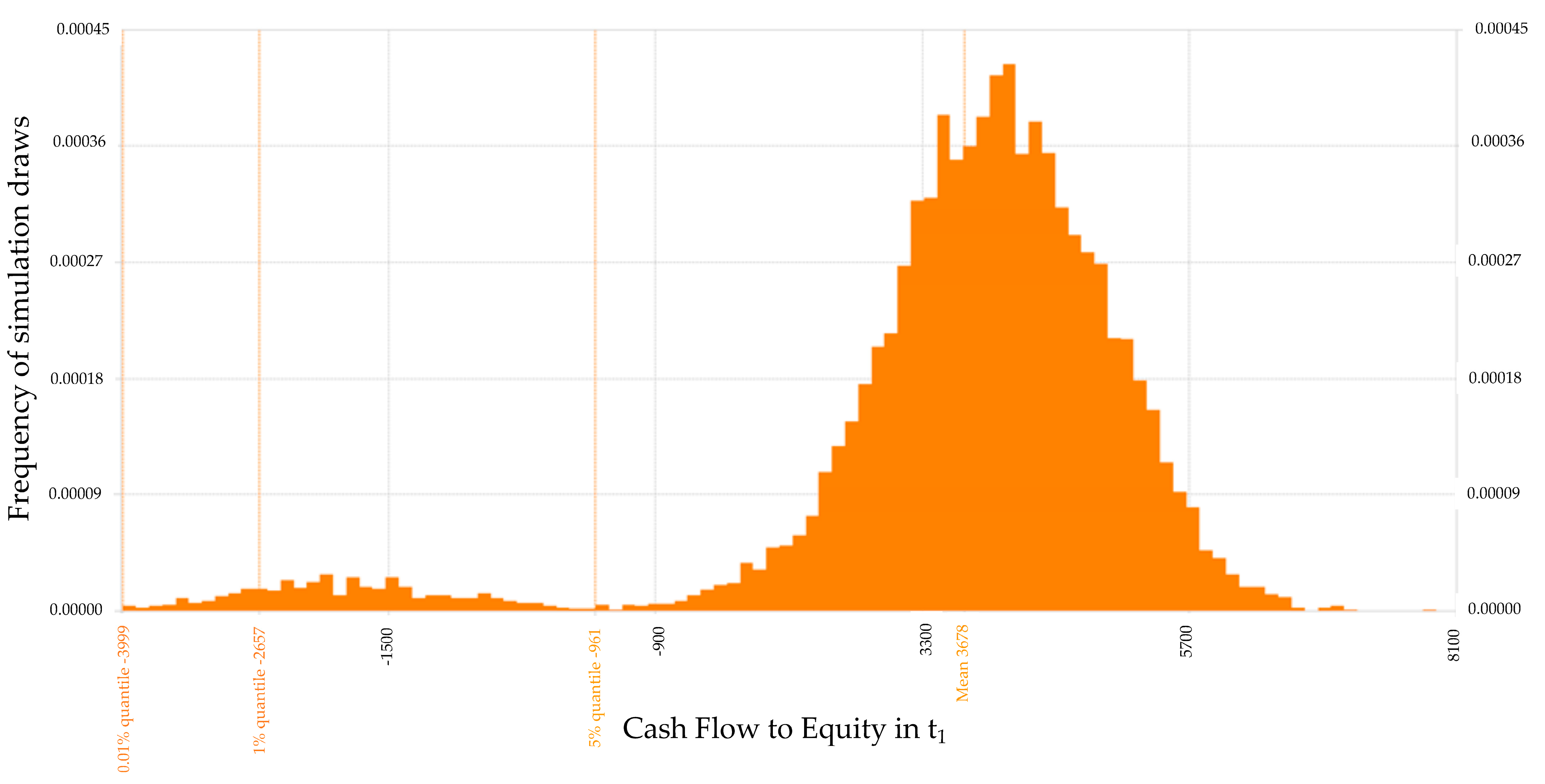Figure 1 shows the result of the simulation for the cash flow to equity of period 1 in the form of a histogram. This shows that the expected value is EUR 3678 billion, and the histogram has a fat tail. This fat tail contains extreme risks that arise from the combination of unfavorable constellations when drawing input parameters from their distribution functions. The extreme negative expressions of the CFtE are shown by $VA{R}_{1-\propto }\left(X\right)=Q_{\alpha }\left(X\right)$ for the 1% and 0.1% quantiles. The values are EUR −2657 million and EUR −3880 million, respectively. These are extremely high deviations from the expected value.

Table 6. Calculation and conversion of position-variant risk measures into position-invariant risk measures.

	Standarddeviation	VaR99%	DVaR99%	CVaR99%	DCVaR99%
Position-variant risk measure		2800		3225
Position-invariant risk measure	1626X		6441	X	6854

shows the values of the standard deviation and for the 1% quantile of the value at risk (VaR), deviation value at risk (DVaR), conditional value at risk (CVaR), and deviation conditional value at Risk (DCVaR). When using the VaR and CVaR, these risk measures have to be converted into DVaR and CVaR to be able to be used in simulation-based valuations.

The formulas for calculating the risk measures are as follows:

$$\sigma \left(X\right)=\sqrt{E(\left(X-E\left(X\right){)}^2\right)}$$

(11)

$$Va{R}_{1-\alpha }\left(X\right)=\left\{\begin{array}{c}\left|Q_{\alpha }\left(X\right)\right|, Q_{\alpha }\left(X\right)<0\\ \\ 0\end{array}\right.$$

(12)

$$DVa{R}_{1-\alpha }\left(X\right)=\left\{\begin{array}{c}\left|Q_{\alpha }\left(X-E\left(X\right)\right)\right|, Q_{\alpha }\left(X-E\left(X\right)\right)<0\\ \\ 0\end{array}\right.$$

(13)

$$CVa{R}_{1-\alpha }\left(X\right)=\left\{\begin{array}{c}\left|E\left(X|X<Q_{\alpha }\left(X\right)\right)\right|, E\left(X|X<Q_{\alpha }\left(X\right)\right)<0\\ \\ 0\end{array}\right.$$

(14)

$$DCVa{R}_{1-\alpha }\left(X\right)=\left\{\begin{array}{c}\left|E\left(X|X<Q_{\alpha }\left[X\right]-E\left(X\right)\right)\right|, E\left(X|X<Q_{\alpha }\left[X\right]-E\left(X\right)\right)<0\\ \\ 0\end{array}\right.$$

(15)

In the next step, we calculate the value of the cash flows for position-invariant risk measures. In addition to the calculated risk measures, we still need values for the market risk premium $\left(E\left({\tilde{r}}_m\right)-r_f\right)$, risk of the market measured as $R\left({\tilde{r}}_m-E\left({\tilde{r}}_m\right)\right)$, and the risk-free interest rate according to Equation (16). Dividing the market risk premium by the market risk yields the price of risk, which is denoted by $\lambda$.

$$\lambda =\frac{\left(E\left({\tilde{r}}_m\right)-r_f\right)}{R\left({\tilde{r}}_m-E\left({\tilde{r}}_m\right)\right)}$$

(16)

$\lambda$ is, in our example,

$$\lambda =\frac{\left(E\left({\tilde{r}}_m\right)-r_f\right)}{R\left({\tilde{r}}_m-E\left({\tilde{r}}_m\right)\right)}=\frac{0.0531}{0.2}=0.2655=26.55\%$$

(17)

The risk-free interest rate is 0.7%. The value of the CFtE of period t(1) has the following values depending on the selected risk measure:

$$\mathrm{Standard}\mathrm{deviation}:V_0\left({\widetilde{CF}}_1\right)=\frac{3.640-1.626·0.2655}{1+0.07}=2999$$

(18)

$$\mathrm{DVaR}{99}_{\%}:V_0\left({\widetilde{CF}}_1\right)=\frac{3.640-6.441·0.2655}{1+0.07}=1804$$

(19)

$$\mathrm{DCVaR}{99}_{\%}:V_0\left({\widetilde{CF}}_1\right)=\frac{3.640-6.865·0.2655}{1+0.07}=1699$$

(20)

For these risk measures, a simulation-based business valuation can be conducted in further steps (see Ernst 2022).

7. Discussion

Risk measures and risk analysis are central components of simulation-based business valuations. The risk concepts discussed in the literature so far are primarily designed for banks and insurance companies. In corporate risk management, not only financial losses but also negative deviations from expected earnings represent central risks. Financial losses can be captured by position-variant risk measures, and negative deviations can be captured from expected returns by position-invariant risk measures.

For position-variant risk measures, a risk axiom system was developed by ADEH, and for position-invariant risk measures, a risk axiom system was developed by RUZ. Position-variant risk measures can easily be transformed into position-invariant risk measures. Only position-invariant risk measures can be used for simulation-based business valuations. This had not yet been demonstrated with such clarity. This means that the VaR, which is popular in practice, must be converted into the DVAR and the CVaR into the DCVaR.

We demonstrated the implementation of the insights gained in a simulation-based business valuation using the valuation equation, which is based on incomplete replication. For this purpose, we used a single-period model. However, this model can also be used without problems for a multiperiod model including terminal value (Ernst 2022).

By answering the above study questions, an important building block in simulation-based business valuations has been laid. Now, further research gaps must be filled to advance the applicability of simulation-based business valuations in business valuation practice.

In addition to the research areas mentioned in the Introduction, the question that needs to be answered in connection with risk measures is how the risk quantities determined via the risk measures can be priced. In the case of standard deviation, this is achieved via the market price of the risk ($\lambda$). We calculate the market price of a risk by putting the market risk premium in relation to the risk of the market. The risk of the market is calculated via the standard deviation of the return of the market. Thus, pricing the risk for the standard deviation risk measure is straightforward. Further consideration is, however, required on how the market price for the risk measures, deviation value at risk, and deviation conditional value at risk can be determined.

Another future area of research is to examine which of the position-independent risk measures used are best suited for which business valuation tasks. Furthermore, whether the results of the simulation-based risk analysis can be empirically validated by using industry data should be analyzed. To establish simulation-based business valuations as a standard business valuation method, further empirical studies with comparisons to other valuation methods need to be conducted.

The research topics mentioned in the Discussion and Introduction are to be successively worked through and solved. These are detailed questions that do not fundamentally call into question the approach of simulation-based business valuations. We see data availability as the main barrier to simulation-based planning and business valuation. To be able to apply the approach, the risks in the company must be known and quantified. These data are usually only held by companies if they are legally obliged to do so or if they attach high importance to risk management in the company. In some countries, e.g., Germany, companies are legally obliged to implement an early risk detection system. This means that the data needed for the simulation-based company evaluation are also available. Another limiting factor is the methodological and quantitative competencies for performing simulations and the associated risk analysis. In the financial industry, these skills are available because they are required by the regulatory framework. These skills are lagging in industrial and service companies.