
Proposal to Extend Access to Loans for Serious Illnesses Using Open Data


Abstract
:1. Introduction
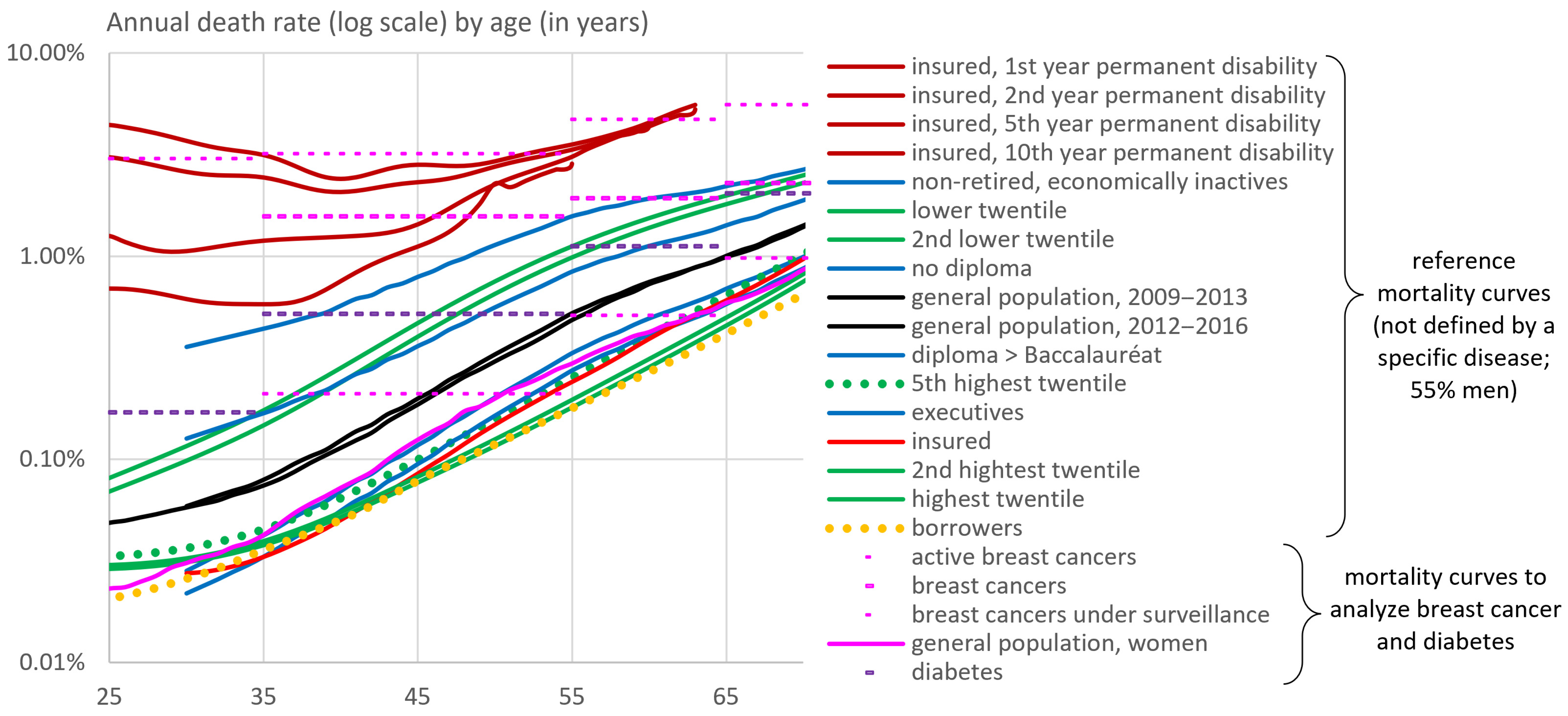
2. Overall Picture Based on French Mortality Benchmarks
3. A Generic Method to Estimate Loan Insurance Premiums for Patients
3.1. Mortality Risk of Patients in the General Population According to Various Risk Factors
3.2. Transposition to Borrowers
3.2.1. Theoretical Considerations and Definition of a Relative Risk Multiplier
3.2.2. Mathematical Definition of the Multiplier and How to Obtain it
- -
- (annual mortality rate of borrowers) and (annual mortality rate in the general population) are functions of age and possibly gender. is an average of placeholder borrower tables calculated by the laboratory; an insurer can apply its own experience table;
- -
- (annual mortality rate of persons with the pathology) depends on age and possibly gender but also on disease-related variables, such as how long ago the diagnosis was made and elements of disease severity;
- -
- (annual mortality rate of borrowers with the pathology) has all these variables;
- -
- is theoretically a function of age, wealth, history of disease, and any other characteristic associated with the loan applicant.
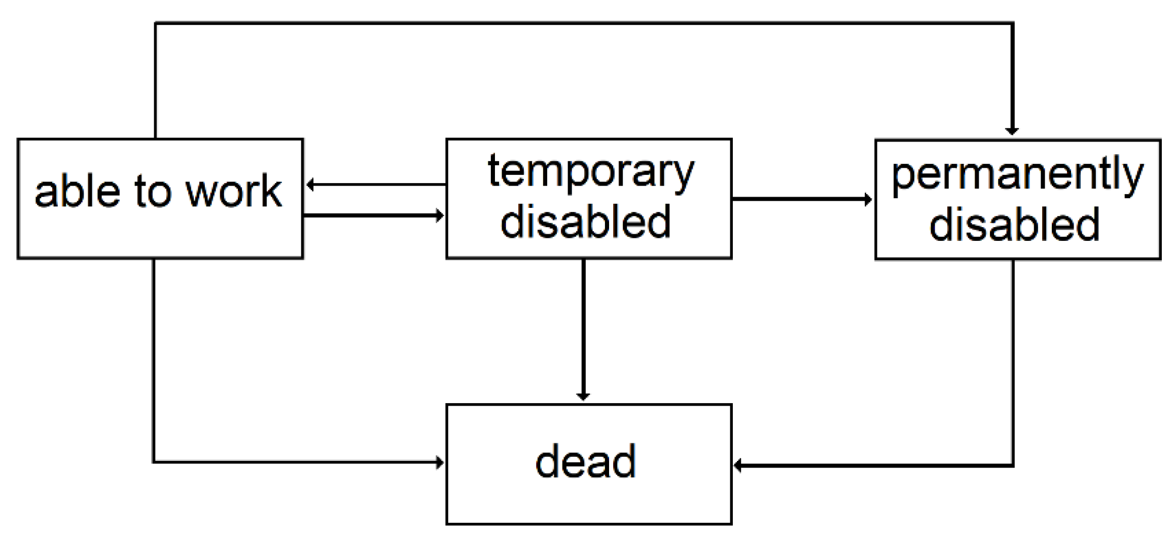
3.2.3. Temporary Disability
- For incidence, we considered a logistic regression giving the annual probability of a work stoppage greater than three days. We chose a logistic regression because this annual incidence is a probability is between 0 and 1, but other models could have been chosen. The three-day threshold was chosen by expert judgement to differentiate temporary disability from pure work stoppage.
- For duration, we considered a gamma regression, giving the duration of a work stoppage greater than 3 days. We chose a gamma regression because it leads to durations that are positive, but other models could have been chosen.
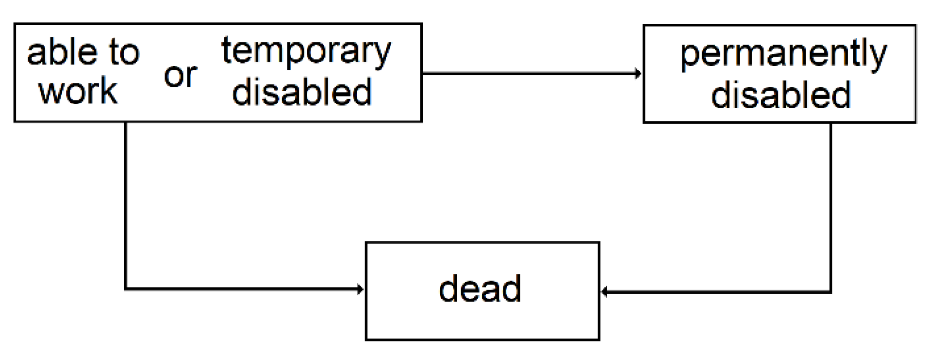
3.2.4. Permanent Disability
3.2.5. Premium Calculation
4. Application to Two Diseases: Breast Cancer and Diabetes
4.1. Breast Cancer
4.1.1. Mortality by Risk Factor
- -
- Age at diagnosis;
- -
- Oestrogen receptor function;
- -
- TNM stage;
- -
- SBR grade.
- -
- Age between 45 and 59;
- -
- Stage T of 1;
- -
- Stage N of 0;
- -
- Stage M of 0;
- -
- Oestrogen receptor dysfunction;
- -
- SBR grade of 1.
- -
- 42.5% were in the higher socio-professional status (SPS+) group defined as “executives, middle professional group, and clerical employees”. Their survival 5 and 7 years post-diagnosis was and , thus on average and ;
- -
- 16.6% did not have a specified SPS;
- -
- 40.9% were in the lower socio-professional status (SPS−) group defined as “famers, artisans, manual workers, unemployed”; Their survival 5 and 7 years post diagnosis was and 69.4%.
4.1.2. Short-Term Disability
- -
- A logistic regression (glm function in R, using “family=binomial(logit)”) yields the following average incidence rate:where is 1 or 0 depending on whether the person was diagnosed with breast cancer or not. We then have and . Our regression found that (more frequent work stoppage at younger ages) and (effect of cancer). was adjusted to match the average frequency of work stoppage in France (Kusnick-Joinville et al. 2006);
- -
- A gamma regression (glm function in R, using “family = Gamman(link = ‘log’)”) yields the following average duration:
4.1.3. Long-Term Disability
- -
- for between and years.
- -
- for beyond years.
4.1.4. Results
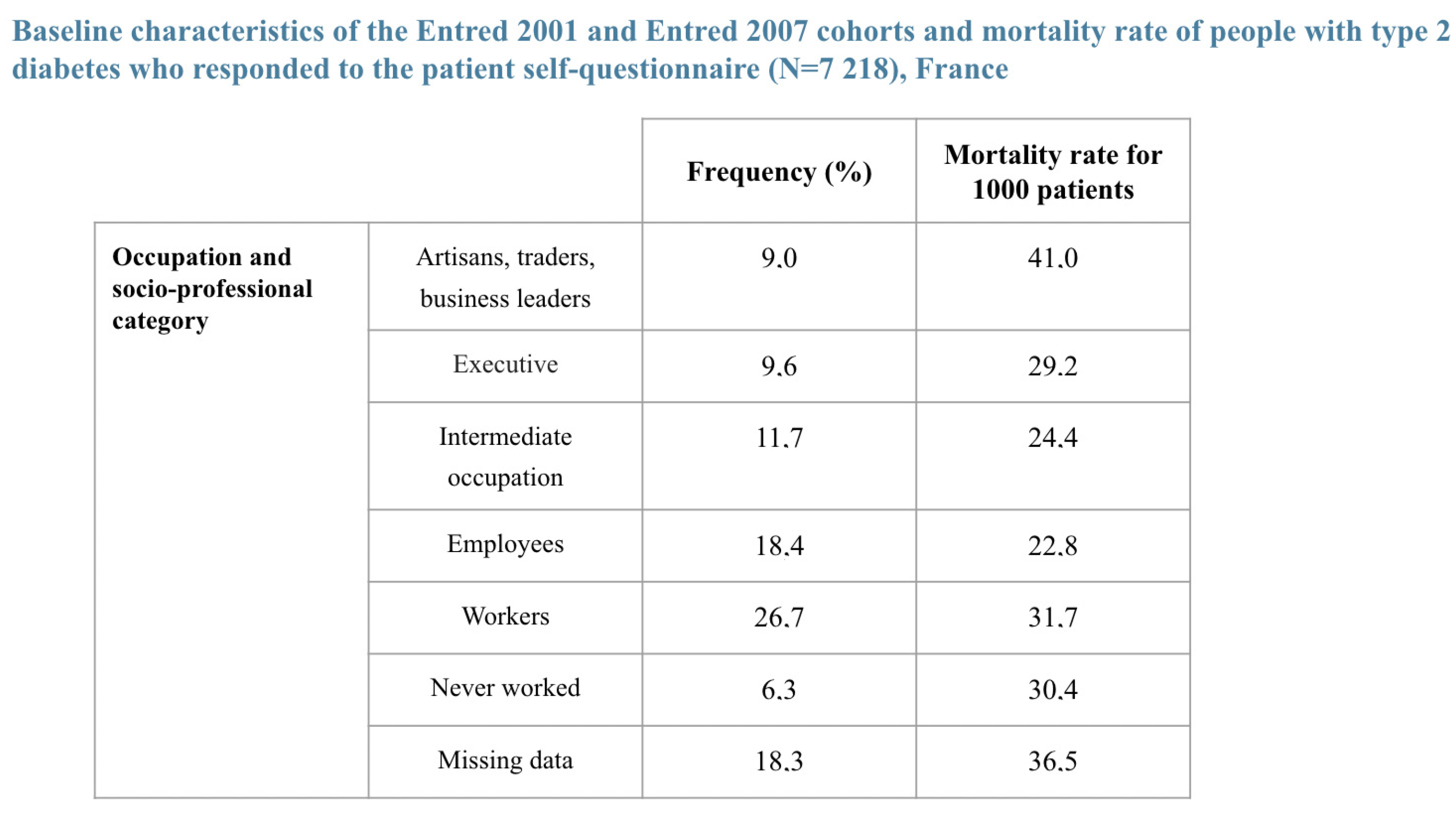
4.2. Diabetes
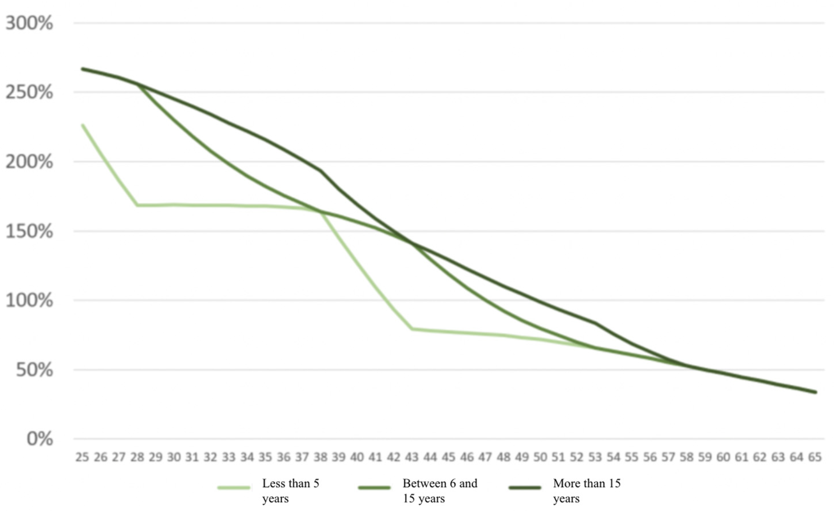
4.2.1. Mortality by Type of Diabetes
4.2.2. Short-Term Disability by Age and Age of Diagnosis
- -
- A logistic regression yields the following average incidence rate:where is 1 or 0 depending on whether the person was diagnosed with breast cancer or not, and is the time since diagnosis (set to 0 for those without type 1 diabetes). We then have and . Regression found (almost no impact of age, overall), (effect of type 1 diabetes), and . was adjusted to match the average frequency of work stoppage in France (Kusnick-Joinville et al. 2006).
- -
- A gamma regression yields the following average duration:
4.2.3. Long-Term Disability
- -
- for between and years.
- -
- for beyond years.
4.2.4. Results
5. Conclusions
Author Contributions
Funding
Institutional Review Board Statement
Informed Consent Statement
Data Availability Statement
Conflicts of Interest
| 1 | For insured risks this gender breakdown is based on expert opinion, as the data at our disposal does not distinguish between the sexes. |
| 2 | Average, maximum and minimum of best estimate actuarial tables among a group of French insurer for the mortality and temporary disability incidence of borrowers. Female risks were obtained by dividing by 1.5 (expert judgement) and male risks where deducted by considering that the tables contained 55% males (expert judgement). |
| 3 | Since the conditional transition probabilities depend on the time spent in the state, semi-Markovian models are better suited, but given the context of this study, this simplification is acceptable. |
| 4 | Surveillance Research Program, National Cancer Institute SEER* Stat software (seer.cancer.gov/seerstat) version 8.3.9. |
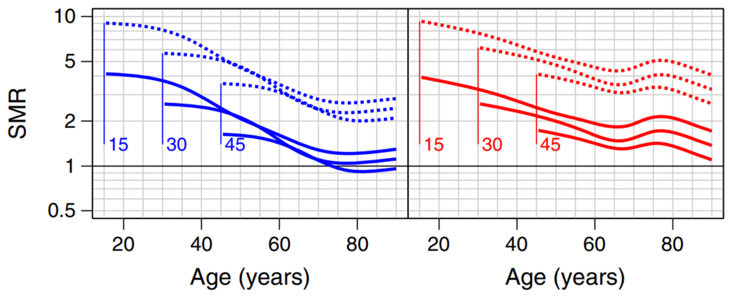
| 5 | In blue and red for men and women respectively. The solid lines represent those without kidney disease. The numbers associated with the curves (15, 30 and 45) are the ages at diagnosis. |
References
- Ameli. 2018a. «Fiches sur les Pathologies» Available on the Website Ameli.fr. Available online: https://assurance-maladie.ameli.fr/etudes-et-donnees/entree-par-theme/pathologies/cartographie-assurance-maladie/donnees/fiches-pathologies/fiches-pathologies (accessed on 5 November 2021).
- Ameli. 2018b. Femmes prises en charge pour cancer du sein actif. Fiche Pathologie. Available online: https://assurance-maladie.ameli.fr/etudes-et-donnees/cartographie-fiche-cancer-sein-femme-actif (accessed on 5 November 2021).
- Ameli. 2018c. Femmes prises en charge pour cancer du sein sous surveillance. Fiche Pathologie. Available online: https://assurance-maladie.ameli.fr/etudes-et-donnees/cartographie-fiche-cancer-sein-femme-sous-surveillance (accessed on 5 November 2021).
- Ameli. 2018d. Diabète. Fiche Pathologie. Available online: https://assurance-maladie.ameli.fr/etudes-et-donnees/cartographie-fiche-diabete (accessed on 5 November 2021).
- Bagui, Hasna. 2013. Refonte des lois de maintien en incapacité temporaire de travail. Mémoire de Master. ISFA. Available online: http://www.ressources-actuarielles.net/C12574E200674F5B/0/CA2755D9E71E059AC1257C78006164B9 (accessed on 20 February 2022).
- Blanpain, Nathalie. 2016. Les inégalités sociales face à la mort. Tables de mortalité par catégorie sociale et par diplôme. INSEE, Résultats. Available online: https://www.insee.fr/fr/statistiques/1893092 (accessed on 20 February 2022).
- Blanpain, Nathalie. 2018. Tables de mortalité par niveau de vie. INSEE, Résultats. Available online: https://www.insee.fr/fr/statistiques/3311422 (accessed on 20 February 2022).
- Cuerq, Anne, Michel Païta, and Philippe Ricordeau. 2008. Points de repère Ameli n°16: Les causes médicales de l’invalidité en 2006. Available online: https://assurance-maladie.ameli.fr/etudes-et-donnees/2008-causes-medicales-invalidite-2006 (accessed on 20 February 2022).
- Dabakuyo, Tienhan Sandrine, Franck Bonnetain, Patrick Roignot, Marie-Laure Poillot, Gilles Chaplain, Thierry Altwegg, Guy Hedelin, and Patrick Arveux. 2008. Population-based study of breast cancer survival in Cote d’Or (France): Prognostic factors and relative survival. Annals of Oncology 19: 276–83. Available online: https://www.annalsofoncology.org/article/S0923-7534(19)41345-8/fulltext (accessed on 20 February 2022).
- Dray-Spira, Rosemary, Tiffany Gary-Webb, and Frederick Brancati. 2010. Educational disparities in mortality among adults with diabetes in the US. Diabetes Care 33: 1200–5. Available online: https://www.ncbi.nlm.nih.gov/pmc/articles/PMC2875423/ (accessed on 20 February 2022).
- Gentil-Brevet, Julie, Marc Colonna, Arlette Danzon, Pascale Grosclaude, Gilles Chaplain, Michel Velten, Franck Bonnetain, and Patrick Arveux. 2008. The influence of socio-economic and surveillance characteristics on breast cancer survival: A French population-based study. British Journal of Cancer 98: 217–24. Available online: https://www.ncbi.nlm.nih.gov/pmc/articles/PMC2359707/ (accessed on 20 February 2022).
- Jørgensen, Marit Eika, Thomas Peter Almdal, and Bendix Carstensen. 2013. Time Trends in Mortality Rates in Type 1 Diabetes from 2002 to 2011. Available online: https://pubmed.ncbi.nlm.nih.gov/23949580/ (accessed on 20 February 2022).
- Kim, Nam Hoon, Tae Joon Kim, Nan Hee Kim, Kyung Mook Choi, Sei Hyun Baik, Dong Seop Choi, Yousung Park, and Sin Gon Kim. 2016. Relative and combined effects of socioeconomic status and diabetes on mortality: A nationwide cohort study. Medicin 95. Available online: https://www.ncbi.nlm.nih.gov/pmc/articles/PMC5265873/ (accessed on 20 February 2022).
- Kusnick-Joinville, Odile, Céline Lamy, Yvon Merlière, and Dominique Polton. 2006. Points de repère Ameli n°5: Déterminants de l’évolution des indemnités journalières maladie. Available online: https://assurance-maladie.ameli.fr/sites/default/files/2006-11_determinants-evolution-indemnites-journalieres-maladie_points-de-repere-5_assurance-maladie.pdf (accessed on 20 February 2022).
- Maruani, Margaret, and Monique Meron. 2012. Un siècle de travail des femmes en France. Paris: La Découverte. [Google Scholar]
- NHIS (National Health Survey). 2016. Centers for Disease Control and Prevention. Available online: https://www.cdc.gov/nchs/nhis/1997-2018.htm (accessed on 20 February 2022).
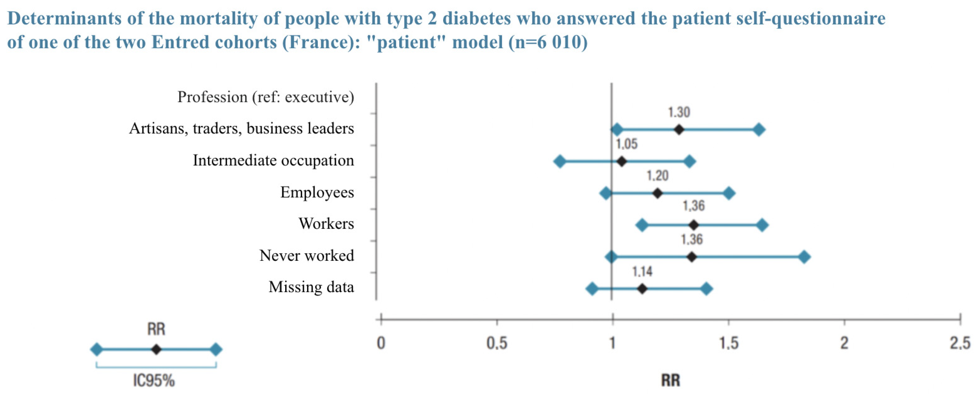
- Piffaretti, Clara, Anne Fagot-Campagna, Grégoire Rey, Juliana Antero-Jacquemin, Aurélien Latouche, and Laurence Mandereau-Bruno. 2016. Déterminants de la mortalité des personnes diabétiques de type 2. Cohortes Entred, France, 2002–2013. Bulletin Epidémiologique Hebdomadaire-BEH, 681–90. Available online: https://www.santepubliquefrance.fr/maladies-et-traumatismes/diabete/documents/article/determinants-de-la-mortalite-des-personnes-diabetiques-de-type-2.-cohortes-entred-france-2002-2013 (accessed on 20 February 2022).
- Ridsdale, B. 2012. Annuity underwriting in the United Kingdom. Note for the International Actuarial Associ-ation Mortality Working Group. Available online: https://www.actuaries.org/CTTEES_TFM/Documents/Zagreb_item19_underwriting_annuities_UK.pdf (accessed on 20 February 2022).
- SEER. 2020. Surveillance, Epidemiology, and End Results (SEER) Program SEER*Stat Database: Incidence—SEER Research Data, 9 Registries, Nov 2020 Sub (1975–2018)—Linked to County Attributes—Time Dependent (1990–2018) Income/Rurality, 1969–2019 Counties, National Cancer Institute, DCCPS, Surveillance Research Program, Released April 2021, Based on the November 2020 Submission. Available online: https://seer.cancer.gov/seerstat/ (accessed on 5 November 2021).
- Tomas, Julien, and Frédéric Planchet. 2014. Prospective mortality table and portfolio experience. In Computational Actuarial Science with R. Edited by A. Charpentier. The R Series; Chapman and Hall: chp. 9. Available online: http://www.ressources-actuarielles.net/gtmortalite (accessed on 20 February 2022).
- Walter, Jeremy, Shona Livingstone, Helen Colhoun, Robert Lindsay, John McKnight, Andrew Morris, John Petrie, Sam Philip, Naveed Sattar, Sarah Wild, and et al. 2011. Effect of socioeconomic status on mortality among people with type 2 diabetes: A study from the Scottish Diabetes Research Network Epidemiology Group. Diabetes Care 34: 1127–32. Available online: https://www.ncbi.nlm.nih.gov/pmc/articles/PMC3114515/ (accessed on 20 February 2022).


| Population with a Pathology | Healthy Population (*) | Relative Mortality Risk Due to Disease | |
|---|---|---|---|
| Higher socio-professional status | |||
| General population |
| Rate (%) | ||
|---|---|---|
| Long-Term Sickness | 3 Years Later | 10 Years Later |
| Multiple sclerosis | 14.0 | 23.4 |
| Incapacitating stroke | 19.8 | 21.9 |
| Severe active rheumatoid arthritis | 10.1 | 7.1 |
| Chronic arteriopathies with ischemic manifestations | 10.6 | 17.0 |
| Coronary artery disease | 9.9 | 15.1 |
| Heart failure, severe heart disease | 9.6 | 14.3 |
| Severe chronic kidney disease and nephrotic syndrome | 7.6 | 13.2 |
| Severe forms of neurological conditions, severe epilepsy | 8.8 | 13.0 |
| Long-term psychiatric conditions | 9.9 | 13.0 |
| Severe chronic respiratory failure | 9.0 | 12.6 |
| Severe ankylosing spondylitis | 8.0 | 12.5 |
| Malignant tumors | 8.4 | 10.8 |
| Severe high blood pressure | 5.1 | 9.8 |
| Chronic active liver disease and cirrhosis | 5.9 | 8.6 |
| Type 1 and 2 diabetes | 3.3 | 7.6 |
| Crohn’s disease and active ulcerative colitis | 2.2 | 4.7 |
| Severe primary immunodeficiency, AIDS | 1.9 | 3.6 |
| 0 | 1 | |
| 0 | 0 | 1 |
| T Stage | N Stage | M Stage | SBR Grade | Oestrogen Receptor Function | m |
|---|---|---|---|---|---|
| 1 | 0 | 0 | 1 | Positive | 2.2 |
| 2 | 0 | 0 | 1 | Positive | 6.4 |
| 3 | 0 | 0 | 1 | Positive | 8.9 |
| 1 | 1 | 0 | 1 | Positive | 5.9 |
| 2 | 1 | 0 | 1 | Positive | 14.6 |
| 3 | 1 | 0 | 1 | Positive | 19.7 |
| 1 | 0 | 0 | 2 | Positive | 5.8 |
| 2 | 0 | 0 | 2 | Positive | 14.4 |
| 3 | 0 | 0 | 2 | Positive | 19.4 |
| 1 | 1 | 0 | 2 | Positive | 13.2 |
| 2 | 1 | 0 | 2 | Positive | 31.0 |
| 3 | 1 | 0 | 2 | Positive | 41.3 |
| 1 | 0 | 0 | 3 | Positive | 8.3 |
| 2 | 0 | 0 | 3 | Positive | 20.0 |
| 3 | 0 | 0 | 3 | Positive | 26.8 |
| 1 | 1 | 0 | 3 | Positive | 18.4 |
| 2 | 1 | 0 | 3 | Positive | 42.4 |
| 3 | 1 | 0 | 3 | Positive | 56.2 |
| 1 | 0 | 0 | 1 | Negative | 3.2 |
| 2 | 0 | 0 | 1 | Negative | 8.5 |
| 3 | 0 | 0 | 1 | Negative | 11.7 |
| 1 | 1 | 0 | 1 | Negative | 7.8 |
| 2 | 1 | 0 | 1 | Negative | 18.9 |
| 3 | 1 | 0 | 1 | Negative | 25.4 |
| 1 | 0 | 0 | 2 | Negative | 7.7 |
| 2 | 0 | 0 | 2 | Negative | 18.7 |
| 3 | 0 | 0 | 2 | Negative | 25.1 |
| 1 | 1 | 0 | 2 | Negative | 17.2 |
| 2 | 1 | 0 | 2 | Negative | 39.7 |
| 3 | 1 | 0 | 2 | Negative | 52.7 |
| 1 | 0 | 0 | 3 | Negative | 10.9 |
| 2 | 0 | 0 | 3 | Negative | 25.8 |
| 3 | 0 | 0 | 3 | Negative | 34.4 |
| 1 | 1 | 0 | 3 | Negative | 23.8 |
| 2 | 1 | 0 | 3 | Negative | 54.1 |
| 3 | 1 | 0 | 3 | Negative | 71.3 |
| T Stage | N Stage | M Stage | SBR Grade | Oestrogen Receptor Function | p |
|---|---|---|---|---|---|
| - | - | 0 | - | - | 13.5 |
| 1 | - | 0 | - | - | 5.8 |
| 2 | - | 0 | - | - | 21.1 |
| 3 | - | 0 | - | - | 31.7 |
| 4 | - | 0 | - | - | 36.7 |
| - | 1 | 0 | - | - | 7.2 |
| - | 0 | 0 | - | - | 24.9 |
| - | - | 0 | 1 | - | 3.5 |
| - | - | 0 | 2 | - | 11.5 |
| - | - | 0 | 3 | - | 21.1 |
| - | - | 0 | - | Negative | 21.4 |
| - | - | 0 | - | Positive | 11.3 |
| South Korea | 108% |
| United States | 111% |
| Scotland | 123% |
| France | 115% |
Publisher’s Note: MDPI stays neutral with regard to jurisdictional claims in published maps and institutional affiliations. |
© 2022 by the authors. Licensee MDPI, Basel, Switzerland. This article is an open access article distributed under the terms and conditions of the Creative Commons Attribution (CC BY) license (https://creativecommons.org/licenses/by/4.0/).
Share and Cite
Planchet, F.; Debonneuil, É.; Péju, M. Proposal to Extend Access to Loans for Serious Illnesses Using Open Data. Risks 2022, 10, 51. https://doi.org/10.3390/risks10030051
Planchet F, Debonneuil É, Péju M. Proposal to Extend Access to Loans for Serious Illnesses Using Open Data. Risks. 2022; 10(3):51. https://doi.org/10.3390/risks10030051
Chicago/Turabian StylePlanchet, Frédéric, Édouard Debonneuil, and Marie Péju. 2022. "Proposal to Extend Access to Loans for Serious Illnesses Using Open Data" Risks 10, no. 3: 51. https://doi.org/10.3390/risks10030051
APA StylePlanchet, F., Debonneuil, É., & Péju, M. (2022). Proposal to Extend Access to Loans for Serious Illnesses Using Open Data. Risks, 10(3), 51. https://doi.org/10.3390/risks10030051