Text Mining for U.S. Pension De-Risking Analysis

Abstract

In the past 30 years, as sponsors of defined benefit (DB) pension plans were facing more severe underfunding challenges, pension de-risking strategies have become prevalent for firms with DB plans to reduce pension-related risks. However, it remains unclear how pension de-risking activities affect firms’ performance, partially due to the lack of de-risking data. In this study, we develop a multi-phase methodology to build a de-risking database for the purpose of investigating impacts of firms’ pension risk transfer activities. We extract company filings between 1993 and 2018 from the SEC EDGAR database to identify different “de-risking” strategies that US-based companies have used. A combination of text mining, machine learning, and natural language processing methods is applied to the textual data for automated identification and classification of de-risking strategies. The contribution of this study is three-fold: (1) the design of a multi-phase methodology that identifies and extracts hidden information from a large amount of textual data; (2) the development of a comprehensive database for pension de-risking activities of US-based companies; and (3) valuable insights to companies with DB plans, pensioners, and practitioners in pension de-risking markets through empirical analysis.

1. Introduction

A defined-benefit pension plan or so-called DB plan is a program that provides employees with pre-established benefits based on factors such as employees’ titles, service years, compensation level, age, etc., throughout their retirement years. Due to the shortfalls in social security, the demand for private retirement funds increased rapidly. DB plan sponsors manage pension assets and are responsible for paying employees’ pension benefits upon their retirement. A DB plan is subject to various risks including investment risk, managerial risk, longevity risk, underfunding risk, and even liquidity risk. If a plan’s pension assets fall short of pension liabilities due to volatile markets, unexpected plan expenditure, or unpredicted longevity improvement, the plan will be identified as an underfunded (or unfunded) pension plan. As a result, sponsoring firms have to either spend their operating cash flows or sell assets to make pension payments when plan beneficiaries request. This negatively affects sponsoring firms and hence creates significant corporate risk.

Many companies, especially those suffering from financial constraints, have been substantially distracted or adversely affected by the pension-related risks. In the last 30 years, defined benefit (DB) pension plan sponsors have faced severe underfunding challenges posed by low interest rates, low returns on investment, and regulatory pressure (e.g., U.S. Department of Labor n.d.). To manage their pension-related risks, companies have been using several de-risking strategies, including pension plan shift, pension plan freeze, pension plan termination, pension buyout, pension buyin, and longevity hedge (Tian and Chen 2020). Despite the high-level demand in pension de-risking and the increasing research interest in this area, there is a lack of comprehensive empirical studies of the various de-risking strategies, mainly due to data unavailability or the difficulty of data acquisition.

Since 1993, public companies have been required by the U.S. Securities and Exchange Commission (SEC) to submit their financial statements to the Electronic Data Gathering Analysis and Retrieval (EDGAR) system. Although these financial statements contain information about companies’ DB pension de-risking activities, it is extremely time-consuming to go through the large number of reports and manually search and classify such information.

In this study, we develop a research methodology that analyzes company filings in the SEC EDGAR database from 1993 to 2018 and extracts key knowledge regarding companies’ pension de-risking activities using text mining, machine learning, and natural language processing (NLP) techniques. The methodology demonstrates a multi-phase process starting with a Web crawler that visits the EDGAR master index website and collects the Web links of all the reports between 1993 and 2018. Then, two levels of document filtering are performed to search the online reports using a list of general pension-related keywords and then an extensive set of keywords and rules related to specific de-risking strategies. Text segments that contain the pre-defined keywords are downloaded to a local disk and then processed, analyzed, and classified using a combination of automated and manual processes.

The rest of the paper is organized as follows. In Section 2, we provide an overview of prior work in the literature that is related to this study. The research methodology is presented in Section 3. We investigate the impacts of pension de-risking on firms’ performance through empirical analysis in Section 4. Section 5 concludes the paper with summaries and contributions.

2. Literature Review

2.1. Research Related to Pension Plan De-Risking Strategies

There is a new but growing body of studies in pension de-risking strategies. Theoretical works may discuss pension risk transfer under hypothetical assumptions, but empirical analyses must rely on data collected from the markets. Therefore, most of the empirical studies focus only on freezes of DB pension plans with limited amount of data and a short time frame. For example, Atanasova and Hrazdil (2010), Comprix and Muller (2011), Choy et al. (2014), and Vafeas and Vlittis (2018) focus their de-risking analysis on pension freezes using data from the periods of 2002–2006, 1991–2008, 2002–2007, and 2000–2015, respectively.

Furthermore, there are very few empirical studies on pension buyouts and buyins in the U.S., despite the fact that the United States is the largest pension fund markets in the world in terms of total pension assets. To the best of our knowledge, the only study that empirically examines these de-risking strategies in the U.S. is from Cantor et al. (2017). They use an event study to investigate 22 buyout and buyin cases between 2012 and 2016. Our research interest is motivated by the demand for large-scale data covering a spectrum of U.S. firms’ de-risking activities so more researchers can conduct empirical studies in this area.

2.2. Text Mining of Financial Documents

Text mining is a type of data mining process with the emphasis on extracting hidden patterns from semi-structured or unstructured data such as documents and Webpages (Türegün 2019). In recent years, text mining has witnessed increased applications in financial domains such as stock market prediction (Nassirtoussi et al. 2014), risk factor identification (Jallan and Ashuri 2020), and financial statement analysis (Türegün 2019) to perform tasks such as document clustering, document classification, text summarization, sentiment analysis, topic detection, and financial decision making.

Researchers have examined various types of textual information including financial news (Schumaker and Chen 2009; Tetlock et al. 2008), online message boards (Das and Chen 2007; Werner and Myrray 2004), and textual content from social media (Bollen and Huina 2011; Vu et al. 2012) for stock market prediction. Machine learning techniques including support vector machine (Schumaker and Chen 2009; Zhai et al. 2007), regression (Hagenau et al. 2013; Tetlock et al. 2008), and decision tree (Huang et al. 2010; Vu et al. 2012) have been used for classification and prediction.

Several studies focus on analyzing companies’ financial reports. For example, Kloptchenko et al. (2004) perform a small-scale analysis of both quantitative and textual data in the quarterly reports of several leading companies in the telecommunication industry. It is concluded that, while the tables with financial numbers indicate how well a company has performed, the linguistic structure and written style of the textual data may reveal the company’s future financial performance. Zheng and Zhou (2012) propose a controlled and knowledge-guided approach that analyzes 8-K, 10-K, and DEF 14A documents from the EDGAR database and produces an evaluation score of a company’s corporate governance process and related policies. They create a collection of knowledge bases and semantic networks to support automated analysis of the documents, based on 200 questions from a corporate governance handbook. Using text mining techniques, Leo (2020) analyzes the annual reports of 26 Global Systemically Important Banks (GSIB) to investigate the extent to which banks make disclosures of their operational resilience risks. Frequency and correlation analysis of different categories of terms reveal that companies make limited disclosures with regard to operational resilience in their annual reports. Jallan and Ashuri (2020) employ text mining and NLP techniques to investigate firms’ disclosures of risk transfer. In particular, they extract disclosure text from 137 firms’ 10-K filings compiled by the SEC from 2006 to 2009 and then identify risk types of different disclosures using text classification techniques.

2.3. Machine Learning in Text Classification

Text classification (also known as text categorization) is the activity of labeling natural language texts with thematic categories from a predefined set (Sebastiani 2002). Since the 1990s, machine learning has become popular and eventually the dominant approach for text classification problems. The most popular machine learning methods for text classification are support vector machines, k-nearest neighbors, Naïve Baysian, and decision trees.

A support vector machine (SVM) is a supervised learning algorithm that is well-suited for text classification because it is robust to overfitting and can scale up to considerable dimensionalities. Unlike other learning methods, little parameter tuning on a validation set is needed when SVM is used (Joachims 1998). Different kernel functions can be plugged into SVM for different types of problems.

K-nearest neighbor (kNN) is another popular learning algorithm for text classification problems. Based on the assumption that similar things exist in close proximity, kNN finds k nearest neighbors of an unlabeled sample and calculates distances between the new data point and each of its neighbors. The data sample is then assigned to the nearest neighboring group (Kumar and Ravi 2016). The selection of the k-value and distance measure can have great impact on the results of the kNN model.

Naïve Baysian (NB) is a probabilistic classifier that models the distribution of documents in each class based on the assumption that the features in a class are independent (Allahyari et al. 2017). As probabilistic models are quantitative in nature, they are not easily interpreted by humans.

A decision tree (DT) text classifier constructs a tree that consists of nodes representing terms, branches labeled by tests on the term weight, and leaves representing categories (Sebastiani 2002). Using a “divide and conquer” strategy, the DT algorithm splits the training data into subgroups based on the tests defined at each branch until a leaf node is reached (Allahyari et al. 2017).

To the best of our knowledge, textual information embedded in SEC filings has not been investigated for pension de-risking research, and machine learning techniques have not been widely applied to such type of documents. In this study, we use various text mining and machine learning methods to analyze SEC financial documents of publicly traded companies from 1993 to 2018 and extract key information related to pension de-risking activities. The focal point of this study is to discover, identify, and categorize de-risking strategies that have been employed by different US-based companies regardless of their industries.

3. Research Methodology

Figure 1 shows the workflow conducted for the present research. Each phase in the workflow is discussed in the following sections.

Figure 1. Research methodology.

3.1. Data Collection

To ensure that all publicly traded companies are completely transparent in their business and financial dealings, the U.S. Securities and Exchange Commission (SEC) requires these companies to file various reports on a regular basis. These reports are available for public access through the Electronic Data Gathering, Analysis, and Retrieval (EDGAR) database (U.S. Securities and Exchange Commission n.d.). In this research, we create a Java Web crawler that visits the master index files of the EDGAR database and downloads web links of all the documents between 1993 and 2018, a total 18.35 million records.

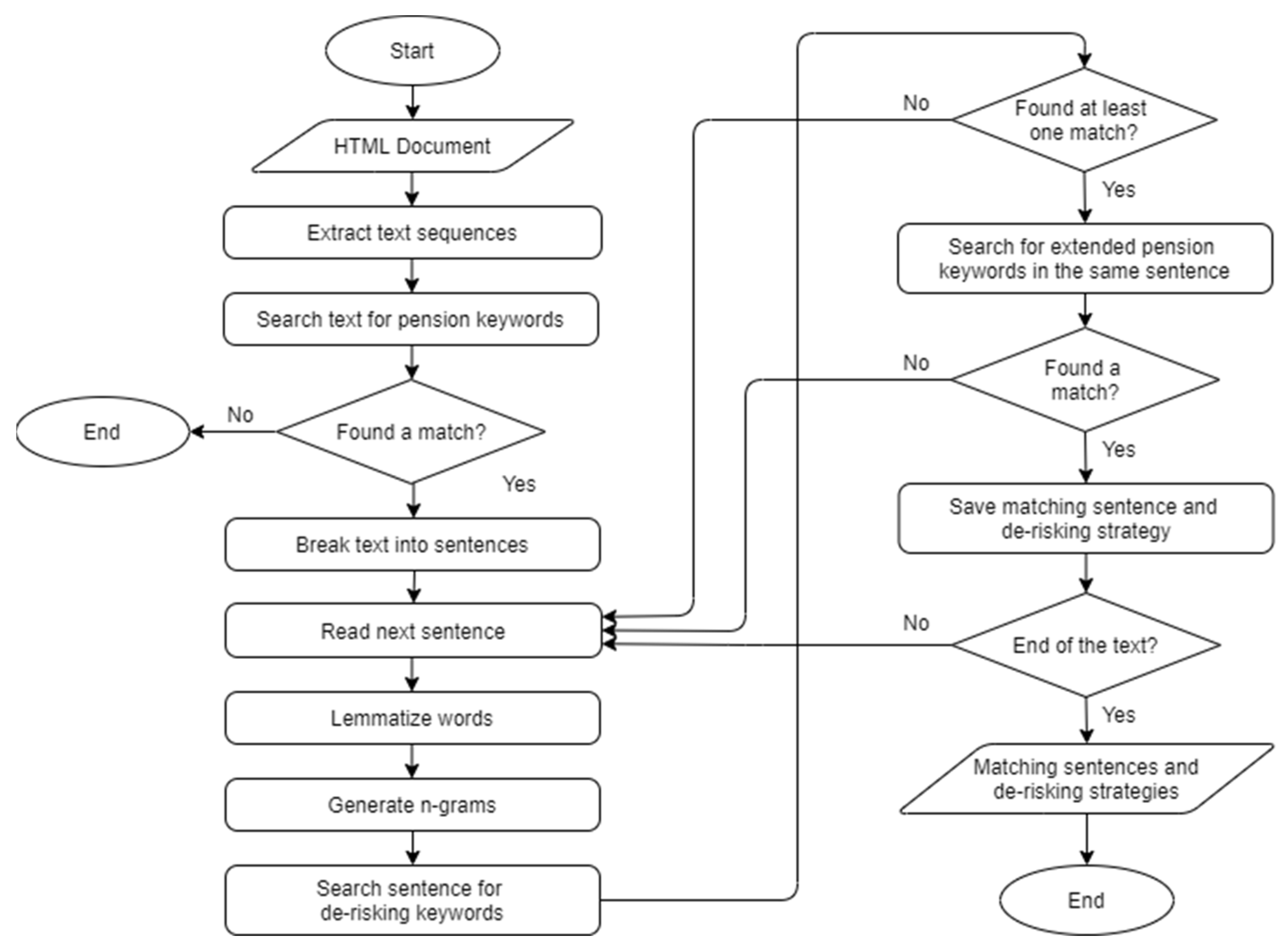
3.2. Level 1 and Level 2 Filters

Our text filtering system is developed using Java, Stanford CoreNLP package, and jsoup to perform two consecutive levels of document filtering. Java is a popular objective-oriented programming language for developing Web systems and software applications. Standford CoreNLP (Stanford NLP Group n.d.) is a Java library that can be used for manipulating natural language such as splitting text into sentences, stemming and lemmatizing words, and generating multi-word phrases (n-grams). As the documents are in HTML format, we also use jsoup library (jsoup: Java HTML Parser n.d.) as the HTML parser.

The process was performed between mid-February and mid-May of 2019 on a high-performance computing cluster hosted at the authors’ university. The center has more than 100 Unix-based compute nodes with 500 TB data storage. During the three-month process, a total of 18.35 million filings were retrieved from the EDGAR database. As shown in Table 1, 1,892,026 and 881,942 filings have been identified as relevant after level 1 filter and level 2 filter, respectively. The total computational time used was 15,002 h and on average, 2.94 s per filing. Since there is one-second wait time between requests sent to the EDGAR Website to avoid the system being denied access, the actual process time per filing is 1.94 s.

Table 1. Computational time and results of level 1 and level 2 processing.

Total No. of Filings Scanned	Total No. of Level 1 Results	Total No. of Level 2 Results	Total Process Time of Level 1 and Level 2 Filters	Average Process Time per Filing
18,351,566	1,892,026	881,942	15,002 h	1.94 s

The flowchart in Figure 2 shows detailed steps of level 1 and level 2 processing. The level 1 filter follows the hyperlinks on the SEC website to search online filings using three basic keywords: “defined benefit”, “pension”, and “retirement”. Documents that contain any of the three keywords are subject to further investigation in the next step. The objective of this step is to conduct a full scan of the 18.35 million filings and eliminate irrelevant documents.

Figure 2. Flowchart of level 1 and level 2 processing.

Following the preliminary scan, the level 2 filter examines the remaining documents in detail and performs rule-based keyword search. An extensive set of keywords and rules are created for identifying and extracting text segments that describe specific de-risking strategies. The objective of the level 2 filter is to assign relevant documents to one or more of the following de-risking strategy categories: shift, freeze, termination, buyout, buyin, and longevity hedge. For each strategy, we define a list of keywords including their synonyms and various linguistic forms, as shown in Table 2. For example, “shift” and “switch” for the shift strategy. We also extend the basic keyword list by including the acronyms of the terms (see Table 3). Then, each keyword from the de-risking-specific list (Table 2) is paired with each of the keywords in the extended basic list (Table 3) to form search rules that require each pair of keywords appearing in the same sentence. For example, for the shift case, one rule states that the keywords “shift” and “defined benefit” must be in the same sentence.

Table 2. De-risking-specific keywords.

Strategy	Search Keywords
Shift	shift, switch
Freeze	freeze
Termination	cease, terminate, termination, wind up
Buyout	buyout, buy-out, buy out
Buyin	buyin, buy-in, buy in
Longevity hedge	longevity

Table 3. Extended basic keywords.

Extended Basic Keywords
DB
DC
Defined benefit
Defined contribution
Pension
Retirement

Using rule-based keyword search, we identified a total of 935,775 documents that contain at least one keyword from each of the two keyword lists in the same sentence. The distribution of these documents across the six de-risking strategies is reported in Table 4. All the sentences that comply with the rules are extracted from each document and saved in a delimited text file along with the metadata of the document such as the year and URL of the report. The potential de-risking strategies indicated by the matching rules are also stored in the file.

Table 4. Distribution of de-risking cases identified by level 1 and level 2 filters.

	Shift	Freeze	Terminate	Buyout	Buyin	LH	Total
Number of cases	20,980	56,302	832,355	19,539	291	6311	935,778

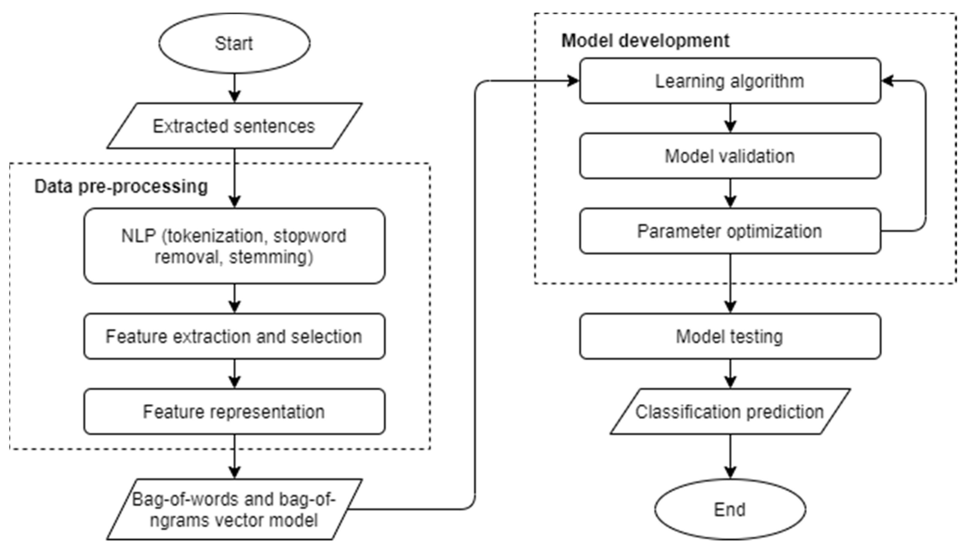
3.3. Machine Learning

One of the biggest challenges of keyword-based text analysis is term variation and ambiguity. Term variation refers to the situation in which a concept is expressed in several different ways and term ambiguity occurs when the same term is used to refer to multiple concepts (Zheng and Zhou 2012). As a result, two texts that contain the same set of keywords may have very different semantic meanings. To alleviate this problem, we employ machine learning techniques to identify true de-risking cases out of the documents identified by the level 2 filter. This process comprises two steps: data pre-processed and model development. Figure 3 shows the flowchart of the machine learning process.

Figure 3. Flowchart of the machine learning process.

3.3.1. Data Pre-Processing

Before textual data can be processed by machine learning algorithms, they need to be transformed from their original unstructured form into a structured data format known as bag-of-words representation (Hotho et al. 2005). Similar to bag-of-words, bag-of-ngrams is also a common approach used in text mining to extract continuous word sequences such as a 2-g (a phrase consisting of two sequential words), 3-g (a phrase consisting of three sequential words), etc. In this study, we extract both bag-of-words and bag-of-ngrams and then create a vector model for each term in the bags with indication of how important the term is to each text segment (consisting of one or more sentences) in the collection. Three steps are performed to obtain the data model: natural language processing, feature extraction and selection, and feature presentation.

Natural language processing (NLP) refers to a set of techniques that are commonly used to interpret human languages in texts and voices. In this study, we first apply tokenization to remove all punctuation marks, replace tabs and other non-text characters with single white spaces, and split the text into a stream of words. Afterwards, we remove stop-words, which are words that frequently appear in the text without having much content information such as “and”, “or”, “the”, etc. (Allahyari et al. 2017). In a natural language, documents often use different forms of a word, such as “terminate”, “terminates”, and “terminating”. For this reason, it is necessary to build the basic forms of words using a method called stemming. A stem is a natural group of words with equal (or very similar) meaning and, after the stemming process, every word is represented by its stem (Hotho et al. 2005). For example, the NLP output of the sentence “the Board took action to terminate the DB plan” consists of the following stems: “board”, “took”, “action”, “termin”, “db”, and “plan”.

Next, we generate n-grams (sequence of n words) from the stems resulted from the previous step. For example, the 2-g and 3-g of the stem list “board”, “took”, “action”, “termin”, “db”, “plan” are as follows:

• 2-g: “board took”, “took action”, “action termin”, “termin db”, “db plan”;
• 3-g: “board took action”, “took action termin”, “action termin db”, “termin db plan”.

All the 2-g and 3-g are combined with the stem list to form features that can be used for machine learning algorithms. As textual data can easily contain many features and the increase in the number of features can decrease the efficiency of most of the learning algorithms (Nassirtoussi et al. 2014), it is necessary to perform feature selection, which is a standard step in the data pre-processing phase of machine learning, especially for data with high dimensionality (Hotho et al. 2005). In this study, we use a simple yet effective method for dimensionality reduction by setting up minimum and maximum frequency limits. Similar to stop-words, regular words occurring very often in the text do not have much value to distinguish documents, while it is unlikely that words occurring very rarely in the text are significantly reverent either (Allahyari et al. 2017). Therefore, both can be removed from the feature list. This method ensures that the most informative words or phrases are selected for the classification task. Appendix B reports the document frequency and total frequency of 2-g and 3-g generated from 800 samples of termination cases. These n-grams appear in 10–90% of all documents.

After features are extracted and selected, they are transformed into a vector space model where each feature (word or phrase) is represented by a numerical value indicating the weight (or importance) of the feature in the document (Allahyari et al. 2017). In this study, we use term frequency-inverse document frequency (TF-IDF), which is a popular term weighting scheme. The TF-IDF value increases proportionally to the number of times a word appears in the document but is offset by the frequency of the word in the document collection (Nassirtoussi et al. 2014). An advantage of the TF-IDF method is that it adds weight to words that frequently appear in a document while taking into consideration the general popularity of some common words in the whole document collection.

3.3.2. Model Training and Testing

After the TF-IDF vector representation of the text is created from the previous step, it is then used to train a machine learning model for text classification. This process consists of the following three steps: algorithm selection, model training, and model testing.

Algorithm Selection

Among the various text classifiers that have been used in the finance domain, the support vector machine (SVM) is the most popular technique because of its high prediction capability (Kumar and Ravi 2016). The extant literature shows that SVM and k-nearest neighbor (kNN) usually deliver top-notch performance, while Naïve Bayes (NB) and decision trees (DT) are less reliable (Hotho et al. 2005). In this step, we compare the performance of SVM, kNN, NB, and DT on a sample dataset using RapidMiner, a commercial data science and machine learning platform (RapidMiner n.d.). The SVM training is carried out with the LIBSVM package (Chang and Lin 2011). A sample of 800 termination cases from 1994 and 1995 is used for the comparison. The sample set has two classes (true and false, or positive and negative) with even distribution. Table 5 shows the training results of LIBSVM classifier in the form of a confusion matrix with values of true positive (TP), true negative (TN), false positive (FP), and false negative (FN).

Table 5. Confusion matrix of LIBSVM with a linear kernel (C = 0.0).

	True Positive	True Negative
Predicted Positive	303 (TP)	16 (FP)
Predicted Negative	45 (FN)	436 (TN)

Based on the confusion matrix drawn from the extant literature (Tang et al. 2009), we calculate the following common performance measures of classification predictions: accuracy, precision, recall, specificity, and F-measure:

$$\mathrm{accuracy}=\frac{\mathrm{TP}+\mathrm{TN}}{\mathrm{TP}+\mathrm{FP}+\mathrm{FN}+\mathrm{TN}}$$

(1)

$$\mathrm{precision}=\frac{\mathrm{TP}}{\mathrm{TP}+\mathrm{FP}}$$

(2)

$$\mathrm{recall}=\frac{\mathrm{TP}}{\mathrm{TP}+\mathrm{FN}}$$

(3)

$$\mathrm{specificity}=\frac{\mathrm{TN}}{\mathrm{TN}+\mathrm{FP}}$$

(4)

$$\mathrm{FMeasure}=\frac{2\times \mathrm{precision}\times \mathrm{recall}}{\mathrm{precision}+\mathrm{recall}}$$

(5)

Accuracy is the ratio of correctly classified samples to the test data, which represents the overall predictive power of the classifier. Precision measures the ratio of true positive sample out of the predicted positive values. Recall (also called sensitivity) is the ratio of true positive samples correctly classified as the positive class, and specificity measures the ratio of true negative samples correctly classified as the negative class. The F-measure is used to integrate precision and recall into a single metric for the convenience of evaluation. Among the four classifiers, as shown in Table 6, SVM performs the best in all the five measures.

Table 6. Performance measures of LIBSVM, kNN, and NB models.

	Accuracy	Precision	Recall	Specificity	F-Measure
Linear SVM (C = 0.0)	92.4%	95.0%	87.1%	96.5%	0.91
kNN (similarity measure = cosine, k = 6)	88.4%	87.2%	85.9%	90.3%	0.87
NB	83.4%	83.9%	76.4%	88.7%	0.80
DT	81.0%	88.3%	64.9%	93.4%	0.75

In linear SVM, there is a penalty parameter C that may affect the prediction accuracy of the model. The penalty parameter determines the trade-off between minimizing the training error and maximizing a classification margin (Tharwat et al. 2017). To test whether a different C value can improve the performance of our learning model, we use grid search to find the best parameter C between 0 and 0.5. The results of the search (Table 7) indicate that the default value 0 achieves the best accuracy. This is consistent with claims from prior research that the default choice of SVM parameter settings has been shown to provide the best effectiveness (Sebastiani 2002).

Table 7. Optimizing penalty parameter C for linear SVM.

Penalty Parameter (C)	Accuracy
0	92.4%
0.05	56.8%
0.10	63.4%
0.15	76.6%
0.20	85.9%
0.25	89.5%
0.30	90.5%
0.35	91.1%
0.40	91.6%
0.45	90.8%
0.50	92.0%

For kNN, we optimize two parameters: k-value and similarity measure (aka distance measure). Using the same sample set, we vary the k-value from 1 to 20 and six similarity measures. As indicated in Table 8, cosine similarity generally performs the best among all the distance measures and the model reaches the highest accuracy (90.00%) when k = 6.

Table 8. Accuracy comparison of different k-values and similarity measures in kNN.

k-Value	Canberra Distance	Chebyshev Distance	Correlation Similarity	Cosine Similarity	Dice Similarity	Euclidean Distance
1	43.5%	79.6%	88.4%	87.8%	89.6%	87.6%
2	56.5%	80.3%	82.8%	86.6%	85.9%	88.0%
3	56.5%	72.5%	87.1%	87.1%	88.3%	89.4%
4	56.5%	71.0%	83.1%	88.6%	86.8%	87.6%
5	56.5%	67.3%	87.3%	89.0%	88.6%	87.8%
6	56.5%	68.4%	86.4%	90.0%	85.5%	88.4%
7	56.5%	65.9%	87.4%	87.5%	88.5%	87.6%
8	56.5%	66.5%	86.3%	89.3%	87.3%	88.4%
9	56.5%	64.6%	87.4%	87.8%	87.6%	87.0%
10	56.5%	65.5%	85.9%	88.0%	87.1%	88.0%
11	56.5%	63.1%	88.1%	88.1%	87.9%	87.3%
12	56.5%	62.9%	86.5%	88.0%	86.9%	88.4%
13	56.5%	62.6%	87.9%	88.9%	87.4%	85.8%
14	56.5%	63.6%	86.9%	88.3%	87.4%	87.9%
15	56.5%	62.5%	89.1%	88.5%	88.5%	88.3%
16	56.5%	62.6%	86.8%	87.8%	87.0%	88.8%
17	56.5%	60.5%	87.1%	87.1%	88.1%	87.5%
18	56.5%	62.0%	86.8%	87.5%	87.4%	88.6%
19	56.5%	60.9%	87.6%	87.5%	87.8%	87.9%
20	56.5%	61.1%	86.1%	87.1%	87.1%	88.1%

Comparing the results and complexity of training the models, SVM outperforms kNN, NB, and DT in terms of both effectiveness and efficiency. Therefore, we choose to focus on SVM for model development and testing.

Model Training

To develop the classifier, we train a collection of 1503 termination cases from 1994, 1995, 2016, and 2018. Two issues need to be addressed during the model training stage. The first is to determine appropriate pruning parameters and the second is to deal with imbalanced data.

In the pre-processing phase, we arbitrarily set up the minimum and maximum limits to remove words that occur very often or very rarely in the text. At this stage, we are interested in finding out whether different pruning parameters will affect the performance of the classifier. We test the following two common pruning settings: (1) below 10% and above 90% and (2) below 5% and above 95%. The results, as shown in Table 9, indicate that less pruning helps improve the performance of the classifier.

Table 9. Comparison of pruning settings and class weighting.

	Accuracy	Precision	Recall	Specificity	F-Measure
Pruning < 10% and > 90%, without class weighting	86.4%	72.6%	78.6%	89.2%	0.75
Pruning < 5% and > 95%, without class weighting	89.3%	79.0%	81.6%	92.1%	0.80
Pruning < 5% and > 95%, with class weighting	93.3%	92.8%	79.6%	97.9%	0.86

The second issue that needs to be addressed is related to the nature of the data set, which is unevenly distributed between the two classes with 402 positive and 1101 negative cases. Compared to other classifiers, SVM is more accurate on moderately uneven data. However, with highly imbalanced data SVM is prone to generating a classifier that has a strong estimation bias toward the majority class, resulting in a drop of performance (Tang et al. 2009). There are a number of approaches to deal with imbalanced data, including oversampling, undersampling, and weighting method. In this study, we apply class weighting to the dataset by setting weights at 2.5 and 1.0 for positive and negative classes, respectively. As shown in Table 9, adding class weights has significantly improved accuracy, precision, specificity, and F-measure. It is also interesting to note that the recall value is slightly lower with class weights than the one without class weights.

Model Testing

Based on the above results, we built a final SVM classifier with class weights and pruning below 5% and above 95%. The model is tested on a much larger dataset with 1139 positive and 5027 negative termination cases from 1996 to 2000. As the dataset is imbalanced, we set the class weights to be 4.4:1.0. The results of the testing are shown in Table 10. The SVM classifier achieved high accuracy, recall, and specificity, but low precision. This indicates that the classifier is effective at identifying as many positive cases as possible (high recall) but tend to misclassify negative cases (low precision).

Table 10. Model testing results.

	Accuracy	Precision	Recall	Specificity	F-Measure
Linear SVM model testing	93.3%	75.0%	95.8%	92.8	0.84

3.4. Level 3 Filter and Manual Process

To further improve the accuracy of identifying true de-risking cases, we perform an additional level of filtering on the text segments extracted from the previous process. Two phrase lists are constructed. The first list, used to narrow the search space of true positive (TP) cases, contains 174 phrases and phrase combinations that often occur in true positive cases. The second list, used to eliminate false positive (FP) cases, contains 119 phrases and phrase combinations that often exist in false positive cases. Using both lists, we apply the level 3 filter to the termination cases (approximately 89% of all the cases) and reduce the search space of termination from 832,355 cases to 40,867 cases, 4.9% of the original size.

To build a highly accurate de-risking database, we manually identify true positive cases from the 40,867 termination cases and cross-validate the results with those generated from the machine learning process.

In addition, we manually review the cases of the other five de-risking strategies except plan termination to remove false positive cases. Table 11 summarizes the numbers of true de-risking cases identified from manual judgement jointly with machine learning methods. The true freeze cases account for 15.4% of the freeze documents retrieved from level 1 and level 2 filters, while less than 1% of the termination, buyout, and longevity hedge documents are identified as true de-risking cases. Overall, our de-risking database consists of total 11,022 de-risking cases of US-based firms for the period 1994–2018.

Table 11. Number of cases by de-risking strategies.

	Shift	Freeze	Terminate	Buyout	Buyin	LH	Total
Cases Identified by Level 1 and Level 2 Filters	20,980	56,302	832,355	19,539	291	6311	935,778
True De-risking Cases	467	8649	1735	138	28	5	11,022
% of True Cases	2.2%	15.4%	0.2%	0.7%	9.6%	0.1%	1.2%

4. Empirical Analysis and Implications

What implications do the pension de-risking data bring to the firms with DB plans? How does pension de-risking affect firms’ performance? In this section, we investigate the impacts of pension risk transfer activities on DB firms’ pension funding status, profitability, credit rating, return volatility, and market value, based on the de-risking data collected through web crawling and text mining. To examine the influence of de-risking at firm level, we first compile the de-risking data (the “True De-risking Cases” row of Table 11) with firms’ financial and stock price data from Compustat, Form 5500, and the Center for Research in Security Prices (CRSP) databases. We then conduct empirical analysis based on the firm-level data for the period 1994–2018.

4.1. Impacts of Pension De-Risking on Firms’ Performance

Denote $\mathcal{D}ℬ$ as the DB firm set that includes all the US-based firms with DB pension plans. The de-risking dummy variable $D$ is defined in $\mathcal{D}ℬ$ as follows:

$D_{it}$equals 1 if firm $i$ has one or more de-risking activities in year $t$. $D$equals 0 for all the observations of the non-derisking firms and the observations of the de-risking firms in the years when they do not conduct any de-risking activity.

Our basic model is as follows:

$$Y_{i,t}={\beta }_0+{\beta }_1{X}_{1,it}+{\beta }_2{X}_{2,it}+\dots +{\beta }_K{X}_{K,it}+{\gamma }_i{I}_i+{\sigma }_t{T}_t+{ϵ}_{it}=\beta X_{it}+{\gamma }_i{I}_i+{\sigma }_t{T}_t+{ϵ}_{it},$$

(6)

where $i=1,\dots ,N;t=1,\dots ,T$, $Y_{it}$ is the dependent variable that measures firms’ performance, $X_{it}={\left[1,X_{1,it},X_{2,it},\dots ,X_{K,it}\right]}^T$ is the explanatory variable vector, $K$ is the number of the predictor variables, $\beta =\left[{\beta }_0,{\beta }_1,\dots ,{\beta }_K\right]$ is the coefficient vector, and the error term ${\epsilon }_{it}~N\left(0,1\right)$. Here, $I_i$ and $T_t$ are the industry and time dummies of firm $i$ and time $t$, respectively. Table 12 reports the results of the generalized linear models (GLM) with $D$ as a key independent variable. The dependent variables $Y$ in columns 2–6 are the pension underfunding ratio, profitability, stock return volatility, credit rating, and excess equity return. Please refer to Appendix A for the descriptions of the variables in Table 12. In all the regressions, we control the time-fixed and industry-fixed effects.

Table 12. Influence of de-risking on firms’ performance.

	Underfunding Ratio	Profitability	Stock Ret Vol.	Credit Rating	Excess Return
$\mathrm{De}-\mathrm{risking}D$	0.024 ***	−0.008 ***	0.009 ***	−0.522 ***	0.011
	(3.640)	(−5.437)	(8.297)	(−7.622)	(1.024)
Total Assets	−0.017 ***	0.004 ***	−0.006 ***	1.114 ***	0.000
	(−11.071)	(11.508)	(−23.394)	(56.191)	(0.027)
Leverage	0.121 ***	−0.099 ***	0.076 ***	−5.232 ***	−0.339 ***
	(5.842)	(−20.951)	(18.399)	(−23.078)	(−8.597)
Profitability	−0.214 ***		−0.091 ***	14.652 ***	0.687 ***
	(−6.155)		(−14.979)	(34.247)	(11.994)
Earnings Volatility	0.042	0.067 **	0.195 ***	−3.173 ***	−1.131 ***
	(0.353)	(2.451)	(8.587)	(−2.044)	(−5.247)
Cash Holding	0.090 ***	0.029 ***	0.031 ***	−5.966 ***	−0.094 **
	(3.112)	(4.419)	(6.374)	(−16.264)	(−2.076)
No-cash Working Capital	0.038 *	0.017 ***	−0.003	−1.617 ***	−0.105 ***
	(1.849)	(3.563)	(−0.702)	(−6.273)	(−3.101)
Tangible Assets	−0.128 ***	−0.052 ***	0.023 ***	0.823 ***	0.036
	(−7.344)	(−13.014)	(7.583)	(4.543)	(1.286)
Capital Expenditure	0.434 ***	0.461 ***	0.048 ***	0.277 ***	−0.705 ***
	(6.972)	(33.076)	(4.438)	(0.390)	(−6.855)
Sales Growth	−0.001	0.001 **	0.002 ***	−0.315 *	0.015 ***
	(−0.307)	(2.151)	(4.888)	(−4.869)	(2.902)
Private Debt	−0.045 *	−0.017	0.009 *	0.481 ***	−0.144 ***
	(−1.762)	(−2.817)	(1.837)	(1.762)	(−3.063)
Constant	0.539 ***	0.112 ***	0.101 ***	3.642 ***	0.047
	(14.596)	(13.307)	(15.907)	(9.411)	(0.771)
Industry-fixed Effect	Yes	Yes	Yes	Yes	Yes
Time-fixed Effect	Yes	Yes	Yes	Yes	Yes
Number of obs.	15,444	16,279	14,023	10,513	13,340
$\mathrm{Adjusted}{R}^2$	0.284	0.308	0.347	0.551	0.062

Note. GLM estimates for the regressions with the de-risking dummy $D$ ($t$ statistics in the parentheses). *, **, and *** denotes significance at the 10%, 5%, and 1% levels, respectively. Year and industry fixed effects are included (but their coefficients are not reported).

The underfunding ratio equals the amount of a firm’s cumulative pension liabilities divided by the amount of cumulative pension assets. The higher the underfunding ratio, the worse a firm’s pension funding status. In Table 12 column 2, the impact of pension de-risking on firm’s pension underfunding ratio is positively significant. This indicates that, although a firm’s poor funding status may motivate the firm to de-risk its pension-related risks, pension de-risking does not directly improve the firm’s pension funding status as expected. De-risking activities typically require an initial cash outlay. As a firm’s cash flows are partially devoted to its pension risk transfer, we observe the firm’s profitability decline (column 3). In column 4, stock return volatility increases after pension de-risking, statistically significant at 1% level. The result implies that de-risking significantly affects firms’ financing decisions as firms reduce pension-related risk and reallocate risk to their core operations. This is the so-called incentive effect (Choy et al. 2014), which claims that firm managers’ incentives become more aligned with stockholders’ after pension de-risking since pension-related risks are transferred to either employees (e.g., shift, freeze, or termination) or a third party (e.g., buyout, buyin, or longevity hedge). Since the incentive effect leads to more risk-taking in firms’ core operations, bondholders may require higher yields to compensate for greater risk perceived through the major performance variables such as profitability and return volatility. As such, the negative effects of pension de-risking on firms’ performance are further reflected in firms’ credit rating downgrades, significant at 1% level (column 5).

However, the estimated coefficient of excess equity return is statistically insignificant, as indicated in column 6 of Table 12. Calculated as a firm’s estimated stock return following Faulkender and Wang (2006) minus the benchmark returns of Fama and French (1993) size and book-to-market matched portfolios in the same year, the equity excess return is a measure of firm value after controlling for the firm’s risk factors. Therefore, after controlling for the firm’s risk factors, the negative impact of pension de-risking on firm value becomes marginal.

Overall, the results in Table 12 show that DB firms’ active risk transfer activities do not immediately benefit firms’ performance. To examine whether the long-term impact of DB pension de-risking are different, we reevaluate the models based on the one-year lead and three-year forward moving average of the dependent variables. Specifically, we rerun (6) with the dependent variable $Y_{i,t+1}$ and $\overline{Y_{i,t+3}}=\frac{1}{3}{\displaystyle \sum }_{\tau =1}^3{Y}_{i,t+\tau }$ in Panel A and Panel B of Table 13, respectively. Again, we include both the time-fixed and industry-fixed effects.

Table 13. Key results of one-year lead and three-year forward moving average regressions.

Panel A: One-Year Lead Dependent Variable
	Underfunding Ratio	Profitability	Credit Rating	Stock Ret Vol.	Excess Equity Return
$\mathrm{De}-\mathrm{risking}D$	0.026 ***	−0.005 ***	−0.519 ***	0.007 ***	0.023 **
	(3.719)	(−3.187)	(−7.322)	(6.261)	(2.264)
Number of obs.	13,800	14,458	9554	12,573	11,998
$\mathrm{Adjusted}{R}^2$	0.271	0.272	0.560	0.326	0.024
Panel B: Three-Year Forward Moving Average Dependent Variable
	Underfunding Ratio	Profitability	Credit Rating	Stock Ret Vol.	Excess Equity Return
$\mathrm{De}-\mathrm{risking}D$	0.027 ***	−0.007 ***	−0.492 ***	0.007 ***	0.012 *
	(4.348)	(−4.677)	(−7.640)	(7.886)	(1.702)
Number of obs.	15,586	16,279	10,883	14,199	13,526
$\mathrm{Adjusted}{R}^2$	0.252	0.310	0.575	0.392	0.063

Note. GLM estimates for the regressions with de-risking dummy $D (t$ statistics in the parentheses). *, **, and *** denote significance at the 10%, 5%, and 1% levels, respectively. Year and industry fixed effects are included (but their coefficients are not reported).

Table 13 reports the key results from the long-term experiments, including the estimated coefficient of the de-risking dummy $D$, the number of observations, and the adjusted $R^2$ for each regression. The long-term impact is roughly consistent with the short-term one, except that the coefficients of the excess equity return are positively significant in both the one-year lead and three-year forward moving average regressions. This indicates that, although pension de-risking may lead to some negative impacts on firms’ short-term performance, in the long run, firms’ active pension risk transfer will effectively improve firm value after controlling for risk factors.

4.2. Implications

Our empirical results send important messages to DB pension plan sponsors, DB firm managers, practitioners, and de-risking product providers. Although pension de-risking may negatively affect DB firms’ operating performance and credit rating in the short run, it can generate positive firm value in the long run. When making pension de-risking decisions, a firm’s manager must be aware of the short-term negative effects of de-risking activities. However, one should not ignore the long-term benefits from such pension risk transfer activities either. At the cost of sacrificing some temporary performance benefits, DB pension de-risking can effectively create firm value in the long run. The empirical analysis also validates our efforts in collecting de-risking data. Without the comprehensive de-risking database, the consequences of pension risk transfer are vague, and managers may be reluctant to conduct pension de-risking as its “side effects” may conceal its long-term benefits to DB firms.

5. Conclusions

In this study, we develop a methodology to process company reports from the SEC EDGAR database and identify different strategies that have been used by US-based publicly traded companies to de-risk their pension plans. Our study makes both theoretical and practical contributions to the extant literature. First, we successfully address the challenges of extracting information from large amount of textual content in SEC filings and dealing with the ambiguity of natural languages. The machine learning techniques applied to the dataset along with rule-based filtering for termination strategies show promising results in identifying true termination cases. For future work, additional filtering constraints such as the maximum length of a sentence and/or the distance between key phases can be imposed to further improve the accuracy of the system. While the methodology is designed for a pension de-risking study, it can be easily adapted to other text classification cases in finance and other business areas.

Second, through the specially designed multiple-stage method, we build a comprehensive de-risking database that consists of different types of de-risking activities of US-based companies which occurred between 1993 and 2018. Our empirical analysis based on the constructed pension de-risking database not only validates the usefulness of the data, but also provides valuable insights to companies with DB plans, pensioners, and practitioners in pension de-risking markets. In addition, we believe that this database can be used to build theoretical models and help researchers conduct further studies to understand firms’ de-risking behaviors and provide related suggestions to regulators.

There are several limitations of this study. First, the testing results of 7262 termination cases show that our SVM classifier is effective at identifying as many positive cases as possible (high recall) but tend to misclassify negative cases (low precision). In other words, it tends to generate more false positive cases than false negative cases. Most recently, there have been developments in NLP with Google’s Transformer-based models as the leading approaches (Vaswani et al. 2017). The transformer models (such as BERT) are based on a deep neural network architecture with a self-attention mechanism for language understanding. Such models have shown performance improvement in classification tasks of social media text (Naseem et al. 2020; Jiang et al. 2019), most notably analyzing sentiment related to COVID-19 pandemic (Ghasiya and Okamura 2021; Singh et al. 2021; Chintalapudi et al. 2021). Due to the limitations of the computing environment, we did not include transformer-based models in this study. It would be interesting to adopt such models in future studies.

Second, as with many other classification problems, the performance of the classifier can be improved by using the most informative features of a specific task. The existing literature suggests that the information gain criterion may be a useful method for feature selection (Joachims 1998) and LSI sometimes perform better than TF-IDF for feature representation (Zhang et al. 2011).

Third, the dataset is highly imbalanced in nature and we have used the weighting mechanism to deal with this issue in the current study. As different methods of handling uneven data could yield different results, future studies should look into other methods such as undersampling, oversampling, and kernel boundary alignment (Tang et al. 2009; Wu and Chang 2005).

References

- Allahyari, Mehdi, Seyedamin Pouriyeh, Mehdi Assefi, Saied Safaei, Elizabeth D. Trippe, Juan B. Gutierrez, and Krys Kochut. 2017. A brief survey of text mining: Classification, clustering and extraction techniques. arXiv arXiv:1707.02919. [Google Scholar]
- Atanasova, Christina, and Karel Hrazdil. 2010. Why do healthy firms freeze their defined-benefit pension plans? Global Financial Journal 21: 293–303. [Google Scholar] [CrossRef]
- Bollen, Johan, and Mao Huina. 2011. Twitter mood as a stock market predictor. Computer 44: 91–94. [Google Scholar] [CrossRef]
- Cantor, David R., Frederick M. Hood, and Mark L. Power. 2017. Annuity buyouts: An empirical analysis. Investment Guides 2017: 10–20. [Google Scholar]
- Chang, Chih-Chung, and Chih-Jen Lin. 2011. LIBSVM: A library for support vector machines. ACM Transactions on Intelligent Systems and Technology 2: 1–27. [Google Scholar] [CrossRef]
- Chintalapudi, Nalini, Gopi Battineni, and Francesco Amenta. 2021. Sentimental analysis of COVID-19 tweets using deep learning models. Infectious Disease Reports 13: 329–39. [Google Scholar] [CrossRef]
- Choy, Helen, Juichia Lin, and Micah S. Officer. 2014. Does freezing a defined benefit pension plan affect firm risk? Journal of Accounting and Economics 57: 1–21. [Google Scholar] [CrossRef]
- Comprix, Joseph, and Karl A. Muller III. 2011. Pension plan accounting estimates and the freezing of defined benefit pension plans. Journal of Accounting and Economics 51: 115–33. [Google Scholar] [CrossRef]
- Das, Sanjiv R., and Mike Y. Chen. 2007. Yahoo! for Amazon: Sentiment extraction from small talk on the web. Management Science 53: 1375–88. [Google Scholar] [CrossRef] [Green Version]
- Fama, Eugene F., and Kenneth R. French. 1993. Common risk factors in the returns on stocks and bonds. Journal of Financial Economics 33: 3–56. [Google Scholar] [CrossRef]
- Faulkender, Michael, and Rong Wang. 2006. Corporate financial policy and the value of cash. Journal of Finance 61: 1957–90. [Google Scholar] [CrossRef]
- Ghasiya, Piyush, and Koji Okamura. 2021. Investigating COVID-19 news across four nations: A topic modeling and sentiment analysis approach. IEEE Access 9: 36645–56. [Google Scholar] [CrossRef] [PubMed]
- Hagenau, Michael, Michael Liebmann, and Dirk Neumann. 2013. Automated news reading: Stock price prediction based on financial news using context-capturing features. Decision Support Systems 55: 685–69. [Google Scholar] [CrossRef]
- Hotho, Andreas, Andreas Nürnberger, and Gerhard Paaß. 2005. A brief survey of text mining. LDV Forum 20: 19–62. [Google Scholar]
- Huang, Chenn-Jung, Jia-Jian Liao, Dian-Xiu Yang, Tun-Yu Chang, and Yun-Cheng Luo. 2010. Realization of a news dissemination agent based on weighted association rules and text mining techniques. Expert Systems with Applications 37: 6409–13. [Google Scholar] [CrossRef]
- Jallan, Yashovardhan, and Baabak Ashuri. 2020. Text mining of the securities and exchange commission financial filings of publicly traded construction firms using deep learning to identify and assess risk. Journal of Construction Engineering and Management 146: 04020137. [Google Scholar] [CrossRef]
- Jiang, Ming, Junlei Wu, Xiangrong Shi, and Min Zhang. 2019. Transformer based memory network for sentiment analysis of web comments. IEEE Access 7: 179942–53. [Google Scholar] [CrossRef]
- Joachims, Thorsten. 1998. Text categorization with support vector machines: Learning with many relevant features. In European Conference on Machine Learning. Berlin and Heidelberg: Springer, pp. 137–42. [Google Scholar]
- jsoup: Java HTML Parser. n.d. Available online: https://jsoup.org/ (accessed on 3 December 2020).
- Klock, Mark S., Sattar A. Mansi, and William. F. Maxwell. 2005. Does corporate governance matter to bondholders? Journal of Financial and Quantitative Analysis, 693–719. [Google Scholar] [CrossRef]
- Kloptchenko, Antonina, Tomas Eklund, Jonas Karlsson, Barbro Back, Hannu Vanharanta, and Ari Visa. 2004. Combining data and text mining techniques for analysing financial reports. Intelligent Systems in Accounting, Finance and Management 12: 29–41. [Google Scholar] [CrossRef]
- Kumar, B. Shravan, and Vadlamani Ravi. 2016. A survey of the applications of text mining in financial domain. Knowledge-Based Systems 14: 128–47. [Google Scholar] [CrossRef]
- Leo, Martin. 2020. Operational Resilience Disclosures by Banks: Analysis of Annual Reports. Risks 8: 128. [Google Scholar] [CrossRef]
- Naseem, Usman, Imran Razzak, Katarzyna Musial, and Muhammad Imran. 2020. Transformer based Deep Intelligent Contextual Embedding for Twitter sentiment analysis. Future Generation Computer Systems 113: 58–69. [Google Scholar] [CrossRef]
- Nassirtoussi, Arman Khadjeh, Saeed Aghabozorgi, Teh Ying Wah, and David Chek Ling Ngo. 2014. Text mining for market orediction: A systematic review. Expert Systems with Applications 41: 7653–70. [Google Scholar] [CrossRef]
- RapidMiner. n.d. Available online: https://rapidminer.com/ (accessed on 3 December 2020).
- Schumaker, Robert P., and Hsinchun Chen. 2009. Textual analysis of stock market prediction using breaking financial news: The AZFin text system. ACM Transactions of Information Systems 27: 1–19. [Google Scholar] [CrossRef]
- Sebastiani, Fabrizio. 2002. Machine learning in automated text categorization. ACM Computing Surveys 34: 1–47. [Google Scholar] [CrossRef]
- Singh, Mrityunjay, Amit Kumar Jakhar, and Shivam Pandey. 2021. Sentiment analysis on the impact of coronavirus in social life using the BERT model. Social Network Analysis and Mining 11: 33. [Google Scholar] [CrossRef]
- Stanford NLP Group. n.d. CoreNLP. Available online: https://stanfordnlp.github.io/CoreNLP/ (accessed on 3 December 2020).
- Tang, Yuchun, Yan-Qing Zhang, Nitesh V. Chawla, and Sven Krasser. 2009. SVMs modeling for highly imbalanced classification. IEEE Transactions on Systems, Man, and Cybernetics, Part B (Cybernetics) 39: 281–88. [Google Scholar] [CrossRef] [Green Version]
- Tetlock, Paul C., Maytal Saar-tsechansky, and Sofus Macskassy. 2008. More than words: Quantifying language to measure firms’ fundamentals. The Journal of Finance 63: 1437–67. [Google Scholar] [CrossRef]
- Tharwat, Alaa, Aboul Ella Hassanien, and Basem E. Elnaghi. 2017. A BA-based algorithm for parameter optimization of Support Vector Machine. Pattern Recognition Letters 93: 13–22. [Google Scholar] [CrossRef]
- Tian, Ruilin, and Jeffrey (Jun) Chen. 2020. De-Risking Strategies of Defined Benefit Plans: Empirical Evidence from the United States. Schaumburg: Society of Actuaries. [Google Scholar]
- Türegün, Nida. 2019. Text mining in financial information. Current Analysis on Economics & Finance 1: 18–26. [Google Scholar]
- U.S. Department of Labor. n.d. Pension Protection Act (PPA). Available online: https://www.dol.gov/agencies/ebsa/laws-and-regulations/laws/pension-protection-act (accessed on 3 December 2020).
- U.S. Securities and Exchange Commission. n.d. About EDGAR. Available online: https://www.sec.gov/edgar/about (accessed on 25 November 2020).
- Vafeas, Nikos, and Adamos Vlittis. 2018. Independent directors and defined benefit pension plan freezes. Journal of Corporate Finance 50: 505–18. [Google Scholar] [CrossRef]
- Vaswani, Ashish, Noam Shazeer, Niki Parmar, Jakob Uszkoreit, Llion Jones, Aidan N. Gomez, Łukasz Kaiser, and Illia Polosukhin. 2017. Attention is all you need. Advances in Neural Information Processing Systems 30: 5998–6008. [Google Scholar]
- Vu, Tien Thanh, Shu Chang, Quang Thuy Ha, and Nigel Collier. 2012. An experiment in integrating sentiment features for tech stock prediction in Twitter. In The Workshop on Information Extraction and Entity Analytics on Social Media Data. Mumbai: The COLING 2012 Organizing Committee, pp. 23–38. [Google Scholar]
- Werner, Antweiler, and Murray Z. Frank. 2004. Is all that talk just noise? The information content of internet stock message board. Journal of Finance 10: 1259–94. [Google Scholar]
- Wu, Gang, and Edward Y. Chang. 2005. KBA: Kernel boundary alignment considering imbalanced data distribution. IEEE Transactions on Knowledge and Data Engineering 17: 786–95. [Google Scholar] [CrossRef] [Green Version]
- Zhai, Yu Zheng, Arthur L Hsu, and Saman K Halgamuge. 2007. Combining news and technical indicators in daily stock price trends prediction. Paer presented at 4th International Symposium on Neural Networks: Advances in Neural Networks, Part III, Nanjing, China, June 3–7; Berlin and Heidelberg: Springer, pp. 1087–96. [Google Scholar]
- Zhang, Wen, Taketoshi Yoshida, and Xijin Tang. 2011. A comparative study of TF*IDF, LSI and multi-words for text classification. Expert Systems with Applications 38: 2758–65. [Google Scholar] [CrossRef]
- Zheng, Ying, and Harry Zhou. 2012. An intelligent text mining system applied to SEC docuemnts. Paper presented at IEEE/ACIS 11th International Conference on Computer and Information Science, Shanghai, China, June 8. [Google Scholar]
Publisher’s Note: MDPI stays neutral with regard to jurisdictional claims in published maps and institutional affiliations. |
© 2022 by the authors. Licensee MDPI, Basel, Switzerland. This article is an open access article distributed under the terms and conditions of the Creative Commons Attribution (CC BY) license (https://creativecommons.org/licenses/by/4.0/).