Abstract
We compare parametric and machine learning techniques (namely: Neural Networks) for in–sample modeling of the yield curve of the BRICS countries (Brazil, Russia, India, China, South Africa). To such aim, we applied the Dynamic De Rezende–Ferreira five–factor model with time–varying decay parameters and a Feed–Forward Neural Network to the bond market data of the BRICS countries. To enhance the flexibility of the parametric model, we also introduce a new procedure to estimate the time varying parameters that significantly improve its performance. Our contribution spans towards two directions. First, we offer a comprehensive investigation of the bond market in the BRICS countries examined both by time and maturity; working on five countries at once we also ensure that our results are not specific to a particular data–set; second we make recommendations concerning modelling and estimation choices of the yield curve. In this respect, although comparing highly flexible estimation methods, we highlight superior in–sample capabilities of the neural network in all the examined markets and then suggest that machine learning techniques can be a valid alternative to more traditional methods also in presence of marked turbulence.
1. Introduction
The term structure of interest rates, whose graphical representation is given by the yield curve, describes the relationship between market interest rates and different times to maturity, and provides an ex–ante measure of the investor’s return in a fixed income market (Saunders and Cornett 2014). Besides, the yield curve contains fundamental information to analyze the economic and financial situation of a country, which can be interpreted in terms of market expectations of monetary policy, economic activity and inflation over short, medium and long–term horizons; for this reason it is often employed to support macroeconomic strategies. Modeling it is therefore fundamental for financial economists and risk managers to define hedging and pricing strategies, as well as to get an effective assessment of portfolio risk (Pereda 2009). Furthermore, yield curves can also provide valuable information as input for financial stability, and banking supervision. Besides, once a nominal yield curve is computed, a term structure of real interest rates and break-even inflation rates can be derived.
When estimating yield curves, an important challenge is that they should reflect as many as possible relevant movements in the underlying term structure of interest rates. In the past decades an extensive literature has been developed accordingly: models based on stochastic processes (Hess 2020), methods relying on splines (Filipović 2009), factor models (Diebold and Rudenbusch 2017) and techniques based on machine learning algorithms (Lopez De Prado 2018), to cite more relevant research strands. Shifting our attention to practical applications, Chakroun and Abid (2014); Ullah and Bari (2018) pinpointed that the great majority of the works focuses on developed countries, mostly the United States and the Eurozone and, on the contrary, relatively lower attention has been paid to emergent markets, despite their growing economic and political weight.
This (relative) lack of contributions on emerging economies is potentially troublesome, as the yield curve of those countries usually exhibits a very volatile behaviour with frequent and marked humps, in contrast to more developed countries whose yield curves are less sensitive. This rationale inspired our study, focused on the group of countries referred by the acronym BRICS (Brazil, Russia, India, China and, since 2010, South Africa) which are actually under the magnifying lens of financial investors as drivers of the globalization process of financial markets (Stuart 2020). The BRICS countries, in fact, have experienced several years of rapid expansion in trade and economic growth: they currently account for nearly a quarter of the world economy. Furthermore, BRICS have set up the New Development Bank (NDB) where those countries address the group’s economic challenges with combined resources. All these elements make the BRICS countries important players in the current pattern of global investment, because they are both the major recipients of foreign direct investments and increasingly important for outward investors. This, in turn, can have deep impact on the exposure to country risk: the economic, political and social contexts can eventually cause losses to foreign investors. After all, BRICS countries inspired many research strands Bekiros and Avdoulas (2020), de Boyrie and Pavlova (2016), Zeb and Rashid (2019), Salisu et al. (2021); however, with the exception of El-Shagi and Jiang (2019) and Caldeira et al. (2020), to the best of our knowledge, there aren’t other works analyzing altogether BRICS yield curves and at the same time investigating on them the interpolation capabilities of various techniques. Such an investigation can be useful under various viewpoints: many central banks use to interpolate yield curves to assess monetary policy measures; in addition such models have an economic interpretation and they can be useful for measuring risk in fixed income portfolios. With this motivation, our paper tried to test whether modeling based on either the parametric or machine learning approach can ensure a streamlined in–sample fitting also for these new world players. To such aim, we compared two alternative methods, the Dynamic Five Factor parametric model (5F–DRF) De Rezende and Ferreira (2013) and the multilayer Feed–Forward Neural Network (FFNNs). The models were chosen among the most performing ones (both parametric and non–parametric). Focusing on the in–sample rather than on the out–of–sample fit was supported by the existing literature, see for instance (Wahlstrom et al. 2021), and (Prasanna and Sowmya 2017) that specifically refer to in–sample fitting of the yield curve. Moreover, as our work examines for the first time the yield curve of all the BRICS at once, it cannot be granted that methods of consolidated use for other countries can adapt so well also to our data, especially in presence of sudden spikes. Working in–sample is therefore nothing but the first step to identify whether those models work well also on emerging countries and which of them is the best model in this task. Answering to those questions, in turn, will allow to better address the forecasting issue for future research.
The 5F–DRF belongs to the factor models family (Diebold and Rudenbusch 2017) which through the past decade have gained wide popularity: its five parameter structure can fit complex curves dynamics, i.e., curves with multiple inflection points. This is a desirable feature as the BRICS exhibit yield curves with humps which are difficult to approximate with more parsimonious models. Moreover, towards this direction, we also worked on the parameters estimation of the 5F–DRF model, introducing a two–step procedure that significantly improves the overall performance of the method, assuring higher model flexibility and better fitting performances also in presence of market turbulence, which is the core issue where often parametric models fail. With regard to machine learning techniques, on the other hand, we focused on Artificial Neural Networks (ANNs) and, in particular, on FFNNs (Dey 2016). Thanks to their ability to bring out knowledge from large and not necessarily homogeneous data sets (Di Franco and Santurro 2020), they have found successful application in a wide variety of fields, including economics and finance Lopez De Prado (2018). The rationale for using FFNNs resides in their flexibility and field–proven ability to replicate yield curves dynamics and stylized facts, as testified by recent works of Rosadi et al. (2011), Vela (2013), Posthaus (2019) and Suimon et al. (2020). The FFNNs capability to manage the ex-ante uncertainty turns out to be of paramount importance within the BRICS bond market where FFNNs are asked to identify the functional form of the yield curve as well as to overcome the limitations of parametric models in presence of multiple humps. Furthermore, the possibility of customizing FFNNs settings for each country, in order to achieve improvements in their fitting ability for all markets is without any doubt an advantage of using this technique.
In short, our work will try to address the following instances. (i) We try to offer a comprehensive view of the yield curves of the BRICS countries through techniques of consolidate use on developed countries markets. (ii) Applying them on the BRICS, that is a set of five emerging countries, in our opinion, should give proof that the results are general and not data–dependent. (iii) An in–depth study of the fitting abilities of those techniques on BRICS yield curves, would also help to better address the forecasting issue for future research.
The remainder of the paper is organized as follows. Section 2 provides a brief description of both the De Rezende–Ferreira model and the neural architecture employed in our simulation; Section 3 contains the results and their discussion; Section 4 concludes and offers some suggestions for further research.
2. Methodology
2.1. The Five Factor De Rezende–Ferreira Model
The De Rezende–Ferreira model assumes to estimate the value of the zero–coupon spot rate depending on a 5-parameter vector and a two dimension array to model the set of humps observable on the yield curve dynamics:
where t is the estimation time, is the maturity over a set of N possible values that can be both fractions and multiples of the year, and are the parameters and decay terms vectors, respectively. In particular, represents the impact of the long–term component which is constant for every maturity; and are the weights associated to the short–term components, and are the weights of the medium–term components. Additionally, and control the convergence speed of the exponential components and determines the maturity at which the medium–term components reach their maximum. By construction, there is a trade-off between the values of , and the effectiveness of the model at long/short term maturities. Big values of (), in fact, result in a slow decay and ensure a better fit at long maturities but not in the short term if marked curvatures are present; conversely small values of () get a quick decay and hence a better fit at short maturities, but not in the long run. Finally, is the error term for all the maturities :, with:
In our study we used a slight modification of the model discussed in De Rezende and Ferreira (2008). We consider the decay components as time–varying parameters and we run a two–step estimation procedure that at each time t finds the optimal pair (, ) as the one associated to the lowest Root Mean Square Error (RMSE). This optimal pair is then employed to get . In contrast to an a priori selection of decay terms, this procedure provides the model with the highest adaptive capability, that is a very desirable feature to use in such a turbulent context like that of the BRICS markets.
For an easier understanding, on following we describe the main steps of the procedure.
- For each market we define the sets = of maturities with and equal to the sets cardinality. In particular, is the lower bound of () and corresponds to the first available maturity of the market, while the upper bound is, at the same time, the lower bound of , that is and it is equal to the straddling maturity between the short and medium–term period. Finally, the upper bound of () is the longest observed maturity. In our study we set = 30 years, as in general there aren’t any bonds traded for longer maturities in the analyzed markets. Values in and ranges between corresponding lower/upper values by proper step sizes and . As the step size can affect the overall performance of the procedure, we tried various step sizes in the range [0.25, 0.75] for and [0.25, 1] for . After extensive simulations we set and .
- For each maturity in the sets and we estimated the parameters and that maximize the medium term component:In this way we get as many curves as the number of maturities.
- For each time t in the time horizon of length T and for every maturity , keep constant and vary to estimate by OLS different array sets ; choose then the set associated to the lowest Sum of Squared Residuals (SSR):with and being the observed and fitted spot rates respectively.
- Repeat Step 3 for all so that there are as many sets of optimal parameters as the values. Then, select the set with the lowest SSR and fit the yield curve at the desired time t:
- Repeat Steps 3–4 for each time t, to get the set of T yield curves fitting and the related time series for all the model parameters.
2.2. Feed Forward Neural Networks
Feed Forward Neural Networks (FFNNs) are non–linear regression tools which do not require any a priori assumption about the functional form or statistical properties of the data set under examination and can be used to identify and model nonlinearity in the data (Hornik et al. 1989). They are made of information processing units (nodes or neurons) arranged into one or more interconnected layers.
Figure 1 shows a graphic representation of an artificial neuron: each input vector is processed by a linear combiner () through the use of a weight vector , and hence transformed with the aid of a proper activation function (usually the sigmoid). At this stage a bias value can be inserted to delay the triggering of the activation function.
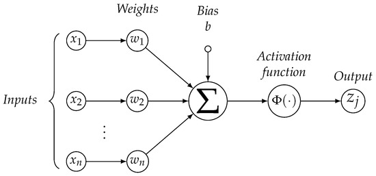
Figure 1.
Representation of a node with n input features.
Nodes are grouped in three types of layers: the Input layer with nodes supplying the input features to next layers consisting of one or more Hidden layers which, in contrast to Input/Output layers, are not in direct contact with either the network input or the output. The response value () is sent either to another hidden layer (if any) or to the Output layer that is the neurons layer which generates the final response of the network.
In order to obtain the desired output, the network must undergo a learning process which identifies the optimal weights configuration (Wilamowski and Irwin 2011): increasing or decreasing the weights values by means of proper learning algorithms changes the strength of nodes connections and directly affects the network capability to learn the input space features. The FFNN makes use of a supervised learning algorithm: information and correct target results are available and presented to the network which tries to define the optimal weights configuration, so that the network response is as close as possible to the correct output. In detail, we used the Backpropagation Algorithm—BPA (Rumelhart et al. 1986). This is an iterative procedure through a certain number of cycles (epochs), each including two phases: a forward stage with the network, initialized at random, generating the output signals (responses), and a backward phase. In the latter the network responses are compared to the target values, the error is back–propagated from the output layer through the hidden ones towards the inputs, and then used to update the networks coefficients to reduce the error at the end of the next forward phase. The process goes on until the optimal combination of weights that minimizes a loss function (e.g., the Mean Squared Error—MSE) is determined according to the gradient descent criterion, so that the estimated output values are the closest to the target output.
3. Empirical Analysis
3.1. Data
Our dataset consists of daily returns for government zero–coupon bonds (ZCB) of the BRICS countries, as summarized in Table 1, where for each country we provided the Start and the End of the observation period, the overall number of observations and the dataset source, that is either TRD (Thomson Reuters Datastream) or CBR (The Central Bank of the Russian Federation).

Table 1.
Dataset description.
As previously said, different maturities could be used to represent the yield curve, depending on the liquidity conditions and availability of information of the analyzed market: for example Diebold and Li (2006) examined maturities from 3 to 120 months (US), while De Rezende and Ferreira (2008) focused on maturities in the range 1 to 60 months (Brazil), and Caldeira et al. (2010) from 1 to 33 months (Brazil). In this work we considered maturities from 3 months (i.e., 0.25 of the year) to 30 years. Combining the available maturities with the observed time we obtained a tensor whose number of rows is equal to the number of analyzed days and with the number of columns equal to the number of maturities. In this way, for each maturity it is possible to observe the evolution of the spot rates time-series: Figure 2a provides an example on the Chinese market with the maturity set at 2, 7 and 15 years respectively; moreover for each day it is possible to extract the yield curve varying the maturities: in Figure 2b we give an example on the Chinese market with t set to 24/01/2005, 09/07/2007, 23/10/2014 and 30/12/2020.
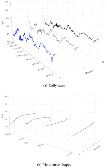
Figure 2.
Behaviour of the daily rates for maturities 2, 7 and 15 years for China in the period 24/01/2005–30/12/2020 (a), and yield curve shapes for China (b) observed in t = 24/01/2005; 09/07/2007; 23/10/2014 and 30/12/2020, respectively.
A closer look to Figure 2a suggests the presence of spikes in the yield curve at various maturities. Such variability is confirmed if we turn to Figure 2b, which offers a snapshot inside how many different behaviours (flat, normal, inverted) the yield curve can show depending on the time assumed as observation point.
Furthermore, varying both t and m for each country it is also possible to build a 3D surface chart as shown in Figure 3 for all the BRICS, where the x-axis reports the time t, the y-axis shows the maturity m expressed in fractions (multiples) of the year and the z-axis the observed level of the interest rate at each time t and for each maturity m.
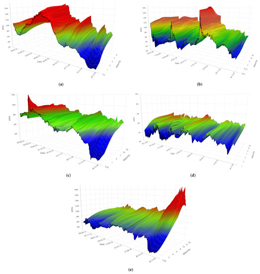
Figure 3.
Zero-Coupon yield surfaces of the BRICS countries in the monitored period. From top to bottom and from left to right, (a) is associated to Brazil, (b) to Russia, (c) to India, (d) to China, (e) to South Africa.
Looking at the shapes of the yield surfaces in Figure 3 suggest that they are the result of quite different instances, that is they have been affected not only by external conditions such as the global crisis or the drop in the commodities demand, but also by internal drivers, such as policy decisions, unemployment and recession in general. In the case of Brazil, (Figure 3a), for instance, pronounced spikes are observable since 2015, when the country began to be interested by a crippling two–year recession (in 2015 and 2016) which was only partially recovered in next years. The booms and busts of the yield surface after 2017 bear witness of the uncertainty dominating the market in those years. In the case of Russia (Figure 3b), on the other hand, the highest turbulence in the yield surface corresponds to the period between 2014 and 2016, when the Russian economy suffered from a currency crisis caused by the collapse of oil prices and the country’s engagement in the conflict with Ukraine. In the case of India (Figure 3c), instead, the mostly flat surface is due to the persistence of economic regression during the whole 2010s. Notably, we can observe an inverted shape of the yield surface corresponding to the period 2012–2014, when India underwent the worst slowdown of the decade in the manufacturing and mining sectors, both of which labour intensive crucial sectors for the growth of other sectors. Conversely, at the end of 2020 the surface turned to a normal behaviour, with lowest (higher) interest rates associated to lower (higher) maturities; how much this stage is solid will depend on the country capability in replying to ongoing inflation of fuel, food prices as well as rising urban unemployment. Similar considerations can be extended to the discussion of the yield surface of South Africa in Figure 3e: in the period 2011–2015, the surface is extremely flat, in connection to higher turbulence in the markets. In this period, in fact, like all economies dependent on commodity prices, the South African economy has been exposed to two highly correlated external shocks: the slowdown in Chinese demand for commodities, which has become the leading destination for South African exports in recent years and the ensuing decline in iron ore. Finally, if we turn the attention to Figure 3d, we can observe that highest variability corresponds to the period from June 2007 to September 2010, when the Chinese financial market faced the Global Financial Crisis, while the flattening of the surface in the following years is due partly to the trade war with the USA and partly to central government driving the country’s transition towards an economy led by consumption and services, rather than one driven by exports and investment.
Overall, we can preliminary conclude that BRICS countries offer the ground for testing the effectiveness of fitting methods in presence of sensitively varying conditions.
For each country data we then run simulations with the 5F–DRF according to the guidelines given in Section 2.1, while for what is concerning the FFNN, the final output was obtained partitioning the countries market data into training (70%), validation (15%) and testing (15%) sets. We defined the number of input, hidden and output neurons depending on the analyzed country; in particular, the quantity of I/O nodes corresponds to the number of available maturities. Regarding the number of intermediate layers and nodes, as there is no a precise rule to select their best combination and the choice is data–dependent (Lantz 2019), we followed a trial and error approach analyzing different configurations (i.e., with one or more hidden layers). The best performance in terms of determination coefficient was obtained with the network architectures summarized in Table 2 for each BRICS country.

Table 2.
Number of layers and neurons for each BRICS country assuring the best fitting performances.
All the FFNNs were trained with the backpropagation learning rule; the learning process was cut after 1000 epochs, i.e., after presenting each training set to the network 1000 times. The fitting accuracy of both models was evaluated comparing the Mean Square Error (MSE) and Root Mean Square Error (RMSE) of both the 5F–DRF model and the FFNN.
3.2. Comparison of the 5F-DRF and FFNN Models Fitting Performances
In this section we present the results of the empirical estimation of the term structure. The analysis was carried out using R 4.0.4 and a freshly-new R package (Castello and Resta 2019) with estimation routines implementing the 5F-DRF model, while the MATLAB R2021a (9.10.0) Neural Network Toolbox was employed to run the FFNNs. All the code is available for download in the Zenodo repository (https://zenodo.org/record/5814658 (accessed on 3 January 2022)).
Table 3 shows the average estimated parameters values for the time–varying 5F–DRF.

Table 3.
Average estimated parameters values for the time–varying 5F–DRF model.
The estimated values emphasise the different role played in the yield curve of BRICS by short/medium and long term components. The value of Brazilian , which addresses the long–term effect, is greater than those of Russia and South Africa by 35% and 24%, and by 96% and 366% than those of India and China, respectively. Clearly, these values reflect the different perception of long–term expectation in the observed countries. Again, if we turn to parameters associated to short term components of the yield curve ( and ), we observe that they differ significantly from one country to another: the scale of values is in the (negative) tenths for Russia, in the dozens for South Africa, in the hundreds for Brazil and China with alternate signs, in the thousands for India. Although so different in scale, values for Brazil, India and China when compared to corresponding , and highlight the importance of short–term expectation in the yield curve of those countries. This aspect is more shaded in the case of South Africa and ever more so for Russia. Mid–term parameters ( and ) are in turn different in scales in various BRICS countries, with higher values associated to India and China, and lower values corresponding to Russia. Overall the estimated values point out how, despite BRICS are often referred as a compact group of countries, the underlying financial and economic drivers substantially differ and they are reflected in the behaviour of the yield curve.
Moving to the results comparison, we obtained a very accurate fit with both the models, as it can be seen in Figure 4, showing the average yield curve against the average fitted ones generated by both the 5F–DRF and the FFNN.

Figure 4.
Average observable yield curve against average yield curves generated by the 5F-DRF (red) and FFNN (blue) models in the BRICS market. From top to bottom and from left to right, (a) is associated to Brazil, (b) to Russia, (c) to India, (d) to China, (e) to South Africa.
At first sight it seems not possible to distinguish the average observable curve from the fit provided by both the 5F–DRF and the FFNN. Besides, a common feature for the two methods seems the capability to fit curves with quite different shapes as well as in different variation ranges. Indeed, despite the fact that all the curves appear to share similar shapes, that is increasing as function of the maturity, the slope of the average yield curve of South Africa in Figure 4e grows faster than in other cases. This curve, in fact, varies in a range of five percentage points while the range of variation of the other yield curve is much smaller. Conversely, the average yield curve of India, in Figure 4c is the flattest one with a range of variation of only 1.2 percentage points. Moreover, both the methods were able to capture different variation ranges: in the interval for Brazil, for Russia, for India, for China and for South Africa. Our first conclusion is that the analysis of the average yield curves does not provide sufficient evidence to uncover which is the best fitting method. Indeed, the lesson learned from this first exploration into the results is that both methods work very well in keeping very different behaviors. In Figure 5, in fact, we offer a direct comparison on the average observable yield curve of the BRICS countries where it is possible to look at the difference in both the variation range and the shape of the curves, as we have already highlighted in the above rows. This feature makes the fitting capabilities of the two methods even more valuable because they were able to capture the dynamics of all the curves, despite the difference in both the maturity spectrum and the steepness of the curve.
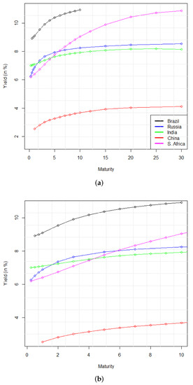
Figure 5.
Plot of the BRICS average observable yield curves (a) and a zoomed-in area (b) which covers the maturity spectrum common to all the examined countries.
In search of more clues, we then turned to analyze the average residuals that are shown in Figure 6.
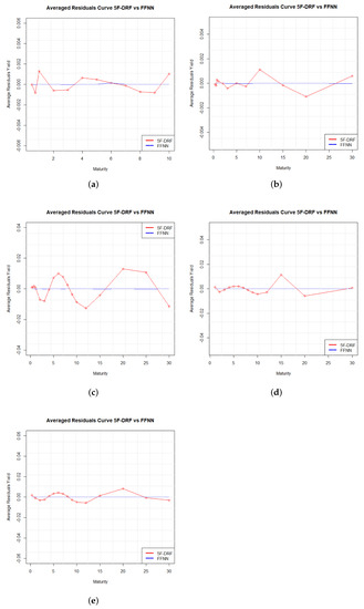
Figure 6.
Average residuals generated by 5F-DRF and FFNN for Brazil (a), Russia (b), India (c), China (d), South Africa (e).
The average residuals are very close to 0 for all the BRICS countries: the range of variation is between for Brazil and Russia while for India, China and South Africa it lies between . These results highlight how both models are characterized by excellent average fitting capabilities. However FFNNs residuals are lower at least by a factor of 100 compared to those of the 5F–DRF model which are characterized by higher oscillations. Taking for example the case of China at the maturity 1 and 30, for m = 1, the errors are equal to and for the 5F–DRF and FFNNs respectively, and equal to and for m = 30.
To evaluate and compare the models fitting abilities we also calculated the MSE and RMSE for the observed yield curves for each maturity, reporting main statistics in Table 4.

Table 4.
Main statistics for MSE and RMSE associated to 5F-DRF and FFNN models applied to the BRICS countries.
The results on the one hand show that both models are characterized by very low values of the MSE. This confirms that on average they both are able to fit the wide variety of shapes exhibited by the yield curves. On the other hand, the results clearly underline the superior fitting abilities of FFNNs on the 5F–DRF model.
Further evidence of the higher fitting abilities of FFNNs is given in the 3D plots shown in Figure 7 and Figure 8 which represent the residuals surface generated by the 5F–DRF and FFNN models respectively, obtained varying both the time t (x–axis) and the maturity m (y–axis). For the FFNN the error surface also includes a zoomed-in area to highlight the residuals magnitude otherwise unobservable at the same scale used to monitor the errors behaviour in the 5F–DRF.
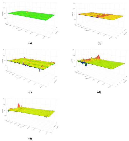
Figure 7.
Surface of daily residuals for the yield curve obtained with the 5F–DRF in the BRICS bond market of Brazil (a), Russia (b), India (c), China (d), South Africa (e).
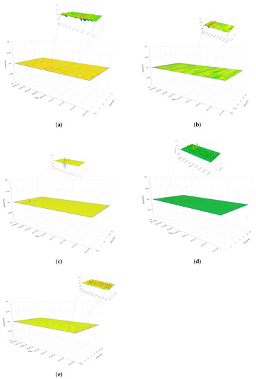
Figure 8.
Surface of daily residuals for the yield curve obtained with the FFNN in the BRICS bond market. As the error surface is very flat, the inset shows a zoomed–in area highlighting the error fluctuations otherwise not visible at the same scale employed to visualize the error surface of the 5F–DRF. From top to bottom and from left to right, (a) is associated to Brazil, (b) to Russia, (c) to India, (d) to China, (e) to South Africa.
In principle, we can conclude that both models provided very good fitting performances. The residuals did not exhibit systematic behaviour, i.e., neither incorrect zeroing or cyclical behaviour caused by wrongly specified models; they took absolute values of very small magnitude with fairly rare spikes mainly concentrated on periods characterized by greater market volatility. In this regard, the error surface of both models contains additional clues leading us to the following conclusions:
- (a) FFNNs perform better than the 5F–DRF model for in sample fitting of the yield curve of the BRICS countries.
- (b) The reason of (a) is in a better adaptability of the FFNN to both internal and external shocks.
The surface generated by the parametric model (5F–DRF), in fact, highlights that more pronounced residuals values are associated to higher market turbulence, as discussed analyzing the yield curve surfaces in Figure 3. This is, for instance, the case of Russia, with maximum values in the error surface of the 5F–DRF corresponding to the period between 2014 and 2016. Again, if we turn the attention to Figure 7d, we can observe that maxima in the error surface correspond to the period from June 2007 to September 2010, when the China was struggling with the Global Financial Crisis. In the case of India (see Figure 7c), instead, we can observe that the whole error surface is disseminated by spikes, mainly concentrated at lower maturities. This clearly indicate an underestimation (overestimation) of the observable values; as a matter of fact, the behaviour of the Indian yield curve at various maturities was a bit trickier to fit than for other countries in the sample: the economic regression probably affected the volatility of financial markets. Similar remarks hold also for South Africa and its error surface in Figure 7e: error peaks raised at the maximum level once again in connection to higher turbulence in the markets. The lone voice in this roundup comes from Brazil, with a flat error surface for the 5F–DRF as it can be seen in Figure 7a, and more pronounced spikes (however not exceeding the range ) in the zoomed–in area of Figure 8a, during the period 2015–2018.
In general, we can conclude that 5F–DRF model suffers for underestimation (overestimation) issue when used to interpolate curves with pronounced oscillations at certain maturities. These are common for parametric model, and even the use of a more efficient parameters estimation can only reduce the error but not at the levels provided by non–linear black box technique like the FFNN. At the same time, in fact, FFNNs provided evidence of being a more flexible tool for in–sample fit of the term structure of interest rates: the residuals generated by the FFNNs are considerably lower, than those of the 5F–DRF and less influenced by the market turbulence in every analyzed situation. They therefore denote a greater ability to replicate almost all the patterns exhibited by the term structure curve, even in cases of strong market fluctuations or downturn.
4. Conclusions
Motivated by the important role played by the term structure of interest rates we investigated and compared the in–sample fitting abilities of two distinct methods, the Five Factor De Rezende–Ferreira (5F–DRF) model and Feed–Forward Neural Networks (FFNNs) when applied to the data of BRICS countries. For the parametric approach we discussed the use of time–varying decay terms to ensure more flexible parameters and hence get higher interpolating performances. Focusing on in–sample rather than out of sample was not limited, in our opinion, as bond prices reflect market participants’ views on interest rate levels in a forward–looking way.
The results may be analyzed under two reading keys. First, we offered a comprehensive study of the BRICS yield curves all at once. In this respect, we outlined how despite BRICS countries are often viewed as a compact set, this is not true, as reflected by the different behaviour of related yield curves. This aspect was accurately kept by the 5F–DRF model, as it can be seen by looking at the average values of estimated parameters: the values, in fact, highlight the different weight associated to short/mid and long–term components of the yield curve. Second, we highlighted very high in–sample fitting capabilities of both the models for all the examined countries. Nevertheless although the 5F–DRF is the most flexible model in the Nelson–Siegel Family and these features have been further enhanced by way of time–varying parameters, the empirical evidence has clearly shown the superior capability of FFNN in interpolating the behaviour of the yield curve; this was also confirmed by comparing the average behaviour of monitored and interpolated yield curves as well as examining the average residuals and the residual surface of both the 5F–DRF and the FFNN. In fact, the FFNN perfectly adapted to all the typical yield curve shapes, even to the most twisted ones with multiple inflection points like in the Indian and Russian case. Moreover FFNNs efficiently replicated all the features of the examined term structures, being flexible enough to overcome the common limitations of parametric models in presence of booms and busts. The greater ability of the FFNN was confirmed by the MSE and RMSE associated to the fit, with values ranging, in the worst case, between for the 5F–DRF and between for the FFNN. Another advantage of FFNNs was related to the estimation process which is less time–consuming than for the 5F–DRF, because it requires a lower amount of parameters during the network calibration process. The possibility of customizing FFNNs settings for each country, in order to achieve improvements in their fitting ability for all markets was without any doubt an additional advantage of using this technique.
Based on the arguments set out above, we therefore conclude that the FFNN is a better and flexible tool for the in–sample fit of the yield curve in all the BRICS markets. Nevertheless we do not underestimate some limitations of our approach and mainly the fact that we performed in–sample fitting. To such aim, future plans include the extension of our conclusions by comparing models performance out–of–sample and a deepest investigation of the potential of our procedure to estimate time–varying parameters in the 5F–DRF compared to alternative solutions discussed in the more recent literature on parametric models.
Author Contributions
Conceptualization, O.C. and M.R.; methodology, O.C. and M.R.; software, O.C.; validation, M.R.; formal analysis, O.C. and M.R.; investigation, O.C. and M.R.; data curation, O.C. and M.R.; writing—original draft preparation, O.C. and M.R.; writing—review and editing, O.C. and M.R.; visualization, O.C. and M.R.; supervision, M.R. All authors have read and agreed to the published version of the manuscript.
Funding
This research received no external funding.
Data Availability Statement
The data are available on Thomson Reuters Datastream and on the website of The Central Bank of the Russian Federation.
Acknowledgments
The authors are thankful to the anonymous referees for their kind comments and suggestions.
Conflicts of Interest
The authors declare no conflict of interest.
Abbreviations
The following abbreviations are used in this manuscript:
| BRICS | Brazil, Russia, India, China, South Africa |
| ANN | Artificial Neural Network |
| FFNN | Feed–Forward Neural Network |
| 5F-DRF | Dynamic De Rezende–Ferreira Five Factor Model |
| BPA | Backpropagation Algorithm |
References
- Bekiros, Stelios, and Christos Avdoulas. 2020. Revisiting the Dynamic Linkages of Treasury Bond Yields for the BRICS: A Forecasting Analysis. Forecasting 2: 102–29. [Google Scholar] [CrossRef]
- Caldeira, João Frois, Guilherme V. Moura, and Marcelo S. Portugal. 2010. Efficient Yield Curve Estimation and Forecasting in Brazil. Revista Economia 11: 27–51. [Google Scholar]
- Caldeira, João Frois, Rangan Gupta, Muhammad Tahir Suleman, and Hudson S. Torrent. 2020. Forecasting the Term Structure of Interest Rates of the BRICS: Evidence from a Nonparametric Functional Data Analysis. Emerging Markets Finance and Trade, 1–18. [Google Scholar] [CrossRef]
- Castello, Oleksandr, and Marina Resta. 2019. DeRezende.Ferreira: Zero Coupon Yield Curve Modelling. R Package Version 0.1.0. Genova: Department of Economics and Business Studies, University of Genova. [Google Scholar]
- Chakroun, Fatma, and Fathi Abid. 2014. A Methodology to Estimate the Interest Rate Yield Curve in Illiquid Market: The Tunisian Case. Journal of Emerging Market Finance 13: 305–33. [Google Scholar] [CrossRef]
- de Boyrie, Maria E., and Ivelina Pavlova. 2016. Dynamic interdependence of sovereign credit default swaps in BRICS and MIST countries. Applied Economics 48: 563–75. [Google Scholar] [CrossRef]
- De Rezende, Rafael Barros, and Mauro S. Ferreira. 2008. Modeling and Forecasting the Brazilian Term Structure of Interest Rates by an Extended Nelson-Siegel Class of Models: A Quantile Autoregression Approach. Resreport, Escola Brasileira de Economia e Finanças. Available online: http://bibliotecadigital.fgv.br/ocs/index.php/sbe/EBE08/paper/download/521/13 (accessed on 8 May 2021).
- De Rezende, Rafael Barros, and Mauro S. Ferreira. 2013. Modeling and Forecasting the Yield Curve by an Extended Nelson-Siegel Class of Models: A Quantile Autoregression Approach. Journal of Forecasting 32: 111–23. [Google Scholar] [CrossRef]
- Dey, Ayon. 2016. Machine Learning Algorithms: A Review. International Journal of Computer Science and Information Technologies 7: 1174–79. [Google Scholar]
- Di Franco, Giovanni, and Michele Santurro. 2020. Machine learning, artificial neural networks and social research. Quality & Quantity 55: 1007–25. [Google Scholar] [CrossRef]
- Diebold, Francis X., and Canlin Li. 2006. Forecasting the term structure of government bond yields. Journal of Econometrics 130: 337–64. [Google Scholar] [CrossRef] [Green Version]
- Diebold, Francis, and Glenn Rudenbusch. 2017. Yield Curve Modeling and Forecasts. Princeton: Princeton University Press. [Google Scholar]
- El-Shagi, Makram, and Lunan Jiang. 2019. Efficient Dynamic Yield Curve Estimation in Emerging Financial Markets. CFDS Discussion Paper Series 2019/4; Kaifeng: Center for Financial Development and Stability at Henan University. [Google Scholar]
- Filipović, Damir. 2009. Term Structure Models. Berlin: Springer. [Google Scholar]
- Hess, Markus. 2020. A pure-jump mean-reverting short rate model. Modern Stochastics: Theory and Applications 7: 113–34. [Google Scholar] [CrossRef]
- Hornik, Kurt, Maxwell Stinchcombe, and Halbert White. 1989. Multilayer feedforward networks are universal approximators. Neural Networks 2: 359–66. [Google Scholar] [CrossRef]
- Lantz, Brett. 2019. Machine Learning with R: Expert Techniques for Predictive Modeling, 3rd ed. Birmingham: Packt Publishing. [Google Scholar]
- Lopez De Prado, Marcos. 2018. Advances in Financial Machine Learning. New York: Wiley. [Google Scholar]
- Pereda, Javier. 2009. Estimacion de la Curva de Rendimiento Cupon Cero para el Perú. Technical Report, Banco Central De Reserva Del Perú. Available online: https://www.bcrp.gob.pe/docs/Publicaciones/Revista-Estudios-Economicos/17/Estudios-Economicos-17-4.pdf (accessed on 28 January 2022).
- Posthaus, Achim. 2019. Yield Curve Fitting with Artificial Intelligence: A Comparison of Standard Fitting Methods with AI Algorithms. Journal of Computational Finance 22: 1–23. [Google Scholar] [CrossRef]
- Prasanna, Krishna, and Subramaniam Sowmya. 2017. Yield curve in India and its interactions with the US bond market. International Economics and Economic Policy 14: 353–75. [Google Scholar] [CrossRef]
- Rosadi, Dedi, Yoga Aji Nugraha, and Rahmawati Kusuma Dewi. 2011. Forecasting the Indonesian Government Securities Yield Curve Using Neural Networks and Vector Autoregressive Model. Technical Report. Yogyakarta: Department of Mathematics, Gadjah Mada University. [Google Scholar]
- Rumelhart, David E., Geoffrey E. Hinton, and Ronald J. Williams. 1986. Learning representations by back-propagating errors. Nature 323: 533–36. [Google Scholar] [CrossRef]
- Salisu, Afees A., Juncal Cuñado, Kazeem Isah, and Rangan Gupta. 2021. Stock markets and exchange rate behaviour of the BRICS. Journal of Forecasting 40: 1581–95. [Google Scholar] [CrossRef]
- Saunders, Anthony, and Marcia Cornett. 2014. Financial Markets and Institutions, 6th ed. New York: The McGraw-Hill/Irwin Series in Finance, Insurance, and Real Estate. [Google Scholar]
- Stuart, Rebecca. 2020. The term structure, leading indicators, and recessions: Evidence from Switzerland, 1974–2017. Swiss Journal of Economics and Statistics 156: 1–17. [Google Scholar] [CrossRef]
- Suimon, Yoshiyuki, Hiroki Sakaji, Kiyoshi Izumi, and Hiroyasu Matsushima. 2020. Autoencoder-Based Three-Factor Model for the Yield Curve of Japanese Government Bonds and a Trading Strategy. Journal of Risk and Financial Management 13: 82. [Google Scholar] [CrossRef]
- Ullah, Wali, and Khadija Malik Bari. 2018. The Term Structure of Government Bond Yields in an Emerging Market. Romanian Journal for Economic Forecasting 21: 5–28. [Google Scholar]
- Vela, Daniel. 2013. Forecasting Latin–American Yield Curves: An Artificial Neural Network Approach. Techreport 761. Colombia: Banco de la República. [Google Scholar]
- Wahlstrom, Ranik Raaen, Florentina Paraschiv, and Michael Schurle. 2021. A Comparative Analysis of Parsimonious Yield Curve Models with Focus on the Nelson-Siegel, Svensson and Bliss Versions. Computational Economics, 1–38. [Google Scholar] [CrossRef]
- Wilamowski, Bogdan M., and David Irwin. 2011. Intelligent Systems, 2nd ed. Boca Raton: CRC Press. [Google Scholar] [CrossRef]
- Zeb, Shumaila, and Abdul Rashid. 2019. Systemic risk in financial institutions of BRICS: Measurement and identification of firm-specific determinants. Risk Management 21: 243–64. [Google Scholar] [CrossRef]
Publisher’s Note: MDPI stays neutral with regard to jurisdictional claims in published maps and institutional affiliations. |
© 2022 by the authors. Licensee MDPI, Basel, Switzerland. This article is an open access article distributed under the terms and conditions of the Creative Commons Attribution (CC BY) license (https://creativecommons.org/licenses/by/4.0/).