Article

Bivariate Copulas Based on Counter-Monotonic Shock Method

by
Farid El Ktaibi
1,†,
Rachid Bentoumi
1,†,
Nicola Sottocornola
1,† and
Mhamed Mesfioui
2,*,†
1
Department of Mathematics and Statistics, Zayed University, Abu Dhabi 144534, United Arab Emirates
2
Département de Mathématiques et d’Informatiques, Université du Québec à Trois-Rivières, Trois- Rivières, QC G8Z 4M3, Canada
*
Author to whom correspondence should be addressed.
These authors contributed equally to this work.
Risks 2022, 10(11), 202; https://doi.org/10.3390/risks10110202
Submission received: 31 August 2022 / Revised: 16 October 2022 / Accepted: 19 October 2022 / Published: 24 October 2022

Abstract

:
This paper explores the properties of a family of bivariate copulas based on a new approach using the counter-monotonic shock method. The resulting copula covers the full range of negative dependence induced by one parameter. Expressions for the copula and density are derived and many theoretical properties are examined thoroughly, including explicit expressions for prominent measures of dependence, namely Spearman’s rho, Kendall’s tau and Blomqvist’s beta. The convexity properties of this copula are presented, together with explicit expressions of the mixed moments. Estimation of the dependence parameter using the method of moments is considered, then a simulation study is carried out to evaluate the performance of the suggested estimator. Finally, an application of the proposed copula is illustrated by means of a real data set on air quality in New York City.

1. Introduction

Copula theories have undergone a spectacular growth in recent decades in view of the increasing importance of modeling and describing different relationships among random variables. New families of copulas have emerged, motivated by the importance of investigating the dependence’s structure in a variety of fields including actuarial science, hydrology, finance and the insurance industry, among others. It is also known, as mentioned in Kole et al. (2007), that copulas offer financial risk managers an interesting mathematical tool to represent complex dependencies in multivariate risk models and are preferable to the traditional, correlation-based approach.
An important bivariate copula model obtained with Sklar’s theorem is the bivariate Marshall–Olkin copula (Nelsen 2006), also known as the generalized Cuadras–Augé family. It is based on the bivariate exponential distribution defined through a stochastic representation interpreted in terms of fatal shocks originally presented in Marshall and Olkin (1967). There is a vast literature documenting the development of generalized families of distributions based on the Marshall and Olkin shock model. See, for instance, Almongy et al. (2021); El-Morshedy et al. (2020); Eliwa and El-Morshedy (2020); Haj Ahmad and Almetwally (2020) and references therein where different extensions of Marshall–Olkin distributions have been provided. It is worth mentioning that the copula of Marshall–Olkin describes only the positive dependence and is neither absolutely continuous nor singular, but rather has both absolutely continuous and singular components. A property that arises naturally in higher dimensions (see Marshall and Olkin 1967).
The aim of this paper is to examine a counterpart of the Cuadras–Augé family of copulas specific for modeling the negative dependence. This can be done by using the counter-monotonic shock method introduced in Genest et al. (2018). More precisely, the proposed bivariate copula is mainly based on the bivariate exponential distribution with negative dependence introduced recently in Bentoumi et al. (2021). This model is perspicuous and interesting in the sense that it fully covers the negative dependence, induced by only one parameter of dependence, and does not impose any restrictions on the correlation structure.
The contribution of this paper is to introduce, in the next section, a new approach-based family of bivariate copulas that span all degrees of negative dependence. In Section 3, we investigate the properties of the suggested family of copulas. We will show that our copula has both absolutely continuous and singular components. We also derive explicit expressions for dependence (concordance) measures, Spearman’s rho, Kendall’s tau and Blomqvist’s beta, and conclude this section by discussing the product moment of the copula. Estimation of the dependence parameter using the method of moments is considered in Section 4. The proposed framework will be illustrated by simulations in Section 5. For the purpose of practical illustration, a real case study is considered in Section 6. Finally, Section 7 provides some concluding remarks and discusses some directions for further research.

2. Proposed Family of Copulas

As noted in the introduction, the purpose of this paper is to present a new strategy to construct a family of copulas that fully covers the negative dependence. To reach this goal, we use the approach taken by Bentoumi et al. (2021), who have introduced a new family of bivariate exponential distribution with given marginal based on the counter-monotonic shock method initiated by Genest et al. (2018).

2.1. The Model

Bentoumi et al. (2021) proposed a negatively dependent family of bivariate exponential distributions described by one dependence parameter θ ( 0 , 1 ) . It has both an absolute continuous part and a singular part, similar to many bivariate exponential models reported in the literature. Specifically, let Λ = ( λ 1 , λ 2 ) , λ i > 0 , i = 1 , 2 and let U be a uniform random variable distributed on [ 0 , 1 ] . Borrowing the notation of Bentoumi et al. (2021), we denote BED ( θ , Λ ) the set of all bivariate exponential random pairs ( X , Y ) , defined as follows.
Definition 1.
Let ( X 1 , X 2 ) and ( Y 1 , Y 2 ) be independent random pairs such that Y i Exp ( θ λ i ) and X i Exp ( λ i ( 1 θ ) ) , i = 1 , 2 . Denote by G i the distribution functions of Y i , i = 1 , 2 , respectively. Assume that
1. 
Y 1 and Y 2 are counter-monotonic; that is, Y 1 = G 1 1 ( U ) and Y 2 = G 2 1 ( 1 U ) .
2. 
X 1 , X 2 and U are independent.
Then
X = min { X 1 , G 1 1 ( U ) } a n d Y = min { X 2 , G 2 1 ( 1 U ) } .
From the stochastic representation (1), we observe that the family BED ( θ , Λ ) approaches the independence case when θ goes to 0 and it reaches the perfect negative dependence described by the Fréchet–Hoeffding lower bound when θ goes to 1. Moreover, it is easily seen that BED ( θ , Λ ) is a family of bivariate exponential random pairs with given marginal distributions, since by construction, X Exp ( λ 1 ) and Y Exp ( λ 2 ) . It is interesting to outline that Equation (1) can be alternatively reformulated as
X = min ln ( U 1 ) λ 1 ( 1 θ ) , ln ( U ) λ 1 θ a n d Y = min ln ( U 2 ) λ 2 ( 1 θ ) , ln ( 1 U ) λ 2 θ ,
where U 1 , U 2 and U are independent and uniformly distributed on [ 0 , 1 ] .
For a nonnegative random vector ( X , Y ) with joint density function f X , Y ( x , y ) and joint survival function S X , Y ( x , y ) , the bivariate hazard rate function (BHRF) is defined as h X , Y ( x , y ) = f X , Y ( x , y ) / S X , Y ( x , y ) . Thus, if ( X , Y ) BED ( θ , Λ ) , then
h X , Y ( x , y ) = λ 1 λ 2 ( 1 θ ) + λ 1 λ 2 θ ( 1 θ ) e λ 1 θ x + e λ 2 θ y 1 ,
for ( x , y ) satisfying e λ 1 θ x + e λ 2 θ y 1 > 0 (see Bentoumi et al. 2021 for more details about the joint density and survival functions).
The surface plots of the bivariate hazard rate function for λ 1 = 0.1 , λ 2 = 0.2 and different values of θ are shown in Figure 1.

2.2. New Approach-Based Copula

The concept of counter-monotonicity can be viewed in relation to the Fréchet–Hoeffding lower bound as described in the definitions below.
Definition 2.
The Fréchet–Hoeffding lower and upper bounds are given by W = max ( u + v 1 , 0 ) and M = min ( u , v ) , respectively.
Definition 3.
The random vector ( X , Y ) with marginal distributions F and G, respectively, is counter-monotonic if there exists a unit uniform random variable U such that ( X , Y ) = d ( F 1 ( U ) , G 1 ( 1 U ) ) . In other words, the joint distribution function of ( X , Y ) is exactly the Fréchet–Hoeffding lower bound.
Let us first recall some standard definitions and properties about copulas, as they can be found for instance in Nelsen (2006). Let X 1 and X 2 be continuous random variables with joint distribution function H and marginal distribution functions F 1 and F 2 , respectively. Then, the random vector X = ( X 1 , X 2 ) has its copula
C X ( u 1 , u 2 ) = H ( F 1 1 ( u 1 ) , F 2 1 ( u 2 ) ) , 0 u 1 , u 2 1 .
Denote H ¯ and F ¯ i = 1 F i , i = 1 , 2 the joint survival function and marginal survival functions, respectively; then, the survival copula is
C ^ X ( u 1 , u 2 ) = H ¯ ( F ¯ 1 1 ( u 1 ) , F ¯ 2 1 ( u 2 ) ) , 0 u 1 , u 2 1 .
The survival copula is a useful tool to describe the structure of dependence among the components and has been widely applied in survival analysis, financial science and reliability engineering.
As is well known, the lower and upper Fréchet–Hoeffding bounds W and M are copulas. Moreover, for any copula C and all ( u , v ) [ 0 , 1 ] 2
W ( u , v ) C ( u , v ) M ( u , v ) .
We end this preliminary by recalling an important copula that we will encounter later, the product copula Π ( u , v ) = u v . In what follows, we study the family of copulas corresponding to the class of distributions, BED ( θ , Λ ) .
Proposition 1.
For every θ ( 0 , 1 ) , the survival copula of ( X , Y ) BED ( θ , Λ ) is given, for all ( u , v ) [ 0 , 1 ] 2 , by
C θ ( u , v ) = u 1 θ v 1 θ W ( u θ , v θ ) .
Proof. 
Let ( X , Y ) BED ( θ , Λ ) and denote by F ¯ and G ¯ the respective survival functions of X and Y. It is well known that the survival copula C θ of ( X , Y ) is exactly the joint distribution of the uniform random pair ( V 1 , V 2 ) = ( F ¯ ( X ) , G ¯ ( Y ) ) . Making use of (2), a bit of algebra yields
V 1 = e λ 1 X = max U 1 1 1 θ , U 1 θ a n d V 2 = e λ 2 Y = max U 2 1 1 θ , ( 1 U ) 1 θ .
Using the fact that U 1 , U 2 and U are independent, it follows that for all ( u , v ) [ 0 , 1 ] 2 ,
C θ ( u , v ) = P V 1 u , V 2 v = P U 1 u 1 θ , U 2 v 1 θ , 1 v θ U u θ = u 1 θ v 1 θ W ( u θ , v θ ) .
This ends the proof of Proposition 1. □
As stated in the introduction, the family of copulas { C θ , θ ( 0 , 1 ) } describes only the negative dependence. Note that the copula C θ is diagonally symmetric since C θ ( u , v ) = C θ ( v , u ) for all ( u , v ) [ 0 , 1 ] 2 . We also remark, in light of Equation (3), that the Fréchet–Hoeffding lower bound copula, W, and the product copula, Π , appear as limiting cases of C θ when θ goes to 0 and 1, respectively. Moreover, the parameter range can be extended to 0 θ 1 and indeed, C 0 = Π and C 1 = W .
Recall the Cuadras–Augé family of copulas (see Cuadras and Augé 1981) defined, for ( θ , u , v ) [ 0 , 1 ] 3 , by
C ˜ θ ( u , v ) = u 1 θ v 1 θ M ( u θ , v θ ) .
One can observe that the family of copulas C θ is expressible in a similar fashion to the Cuadras–Augé family of copulas, involving the Fréchet lower bound rather than the upper bound.
It is worth mentioning here that the family of copulas C θ has been introduced previously in the literature. It can be easily deduced, for instance, from Equation (1) in Dolati et al. (2014), Example 3 in Durante (2009), Proposition 4.1 of Khoudraji (1995) or Theorem 2.1 of Liebscher (2008). Nevertheless, we are not aware of any published work where its construction was based on a counter-monotonic shock model and consequently its corresponding stochastic representation (4). Indeed, the latter representation will provide a useful and easy-to-implement algorithm for generating data from the copula C θ :
  • Generate three independent values u 1 , u 2 and u 3 from uniform [0, 1].
  • Set u = max u 1 1 1 θ , u 3 1 θ and v = max u 2 1 1 θ , ( 1 u 3 ) 1 θ .
  • The desired pair is ( u , v ) .
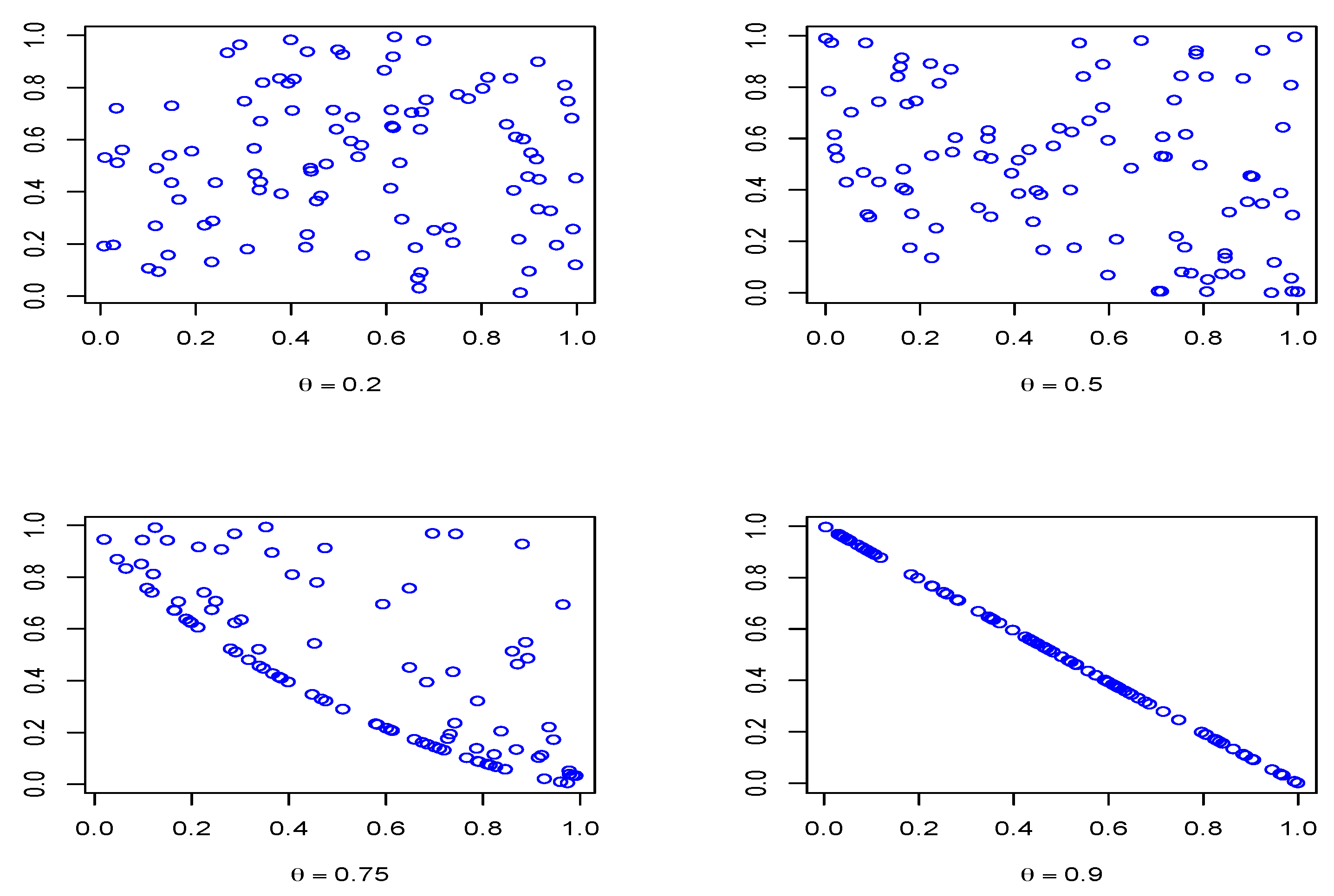
Figure 2 illustrates scatterplots for simulations of the proposed family of copulas C θ , each using 100 pairs of points generated by the above algorithm for different values of θ .
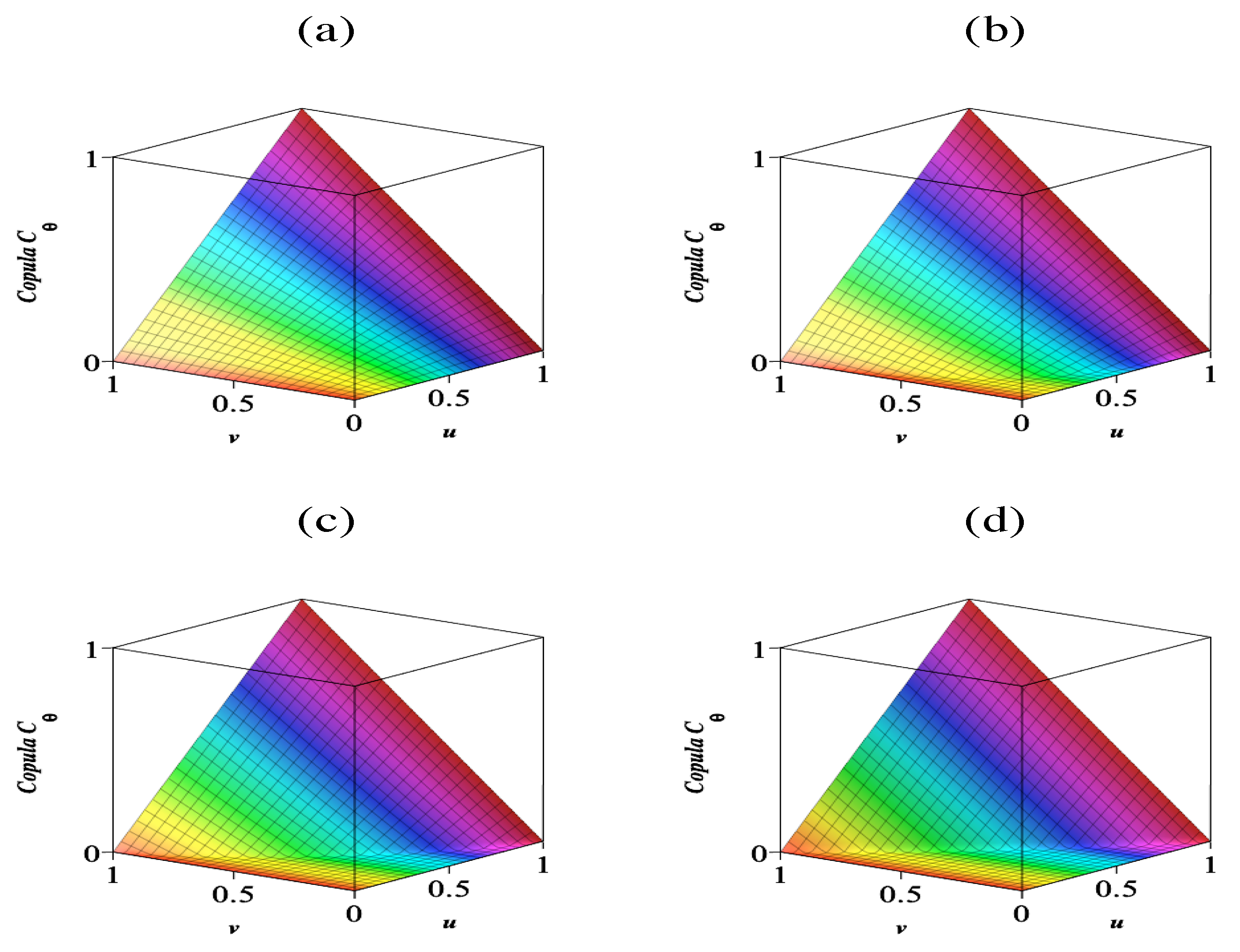
Proposed copula C θ ( u , v ) based on different values of θ is displayed in Figure 3.

3. Properties of the Copula C θ

The following section will be devoted to investigating the properties of the family of copulas C θ . We first present the singular and the absolutely continuous components of the copula and then derive the corresponding copula density function. The concordance measures of C θ , namely Spearman’s rho and Kendall’s tau, will be addressed and expressed succinctly in terms of the beta function. We conclude by analyzing the product moments of the copula that will be exploited in the next section.

3.1. Singularity

Analogously to the Marshall–Olkin copula, the proposed copula C θ is neither absolutely continuous nor singular, but rather has both absolutely continuous and singular components. These two parts involved the incomplete beta function B ( x , a , b ) defined by
B ( x , a , b ) = 0 x t a 1 ( 1 t ) b 1 d t a , b , x > 0 .
Recall that the incomplete beta function satisfies the following useful equation
B ( x , a + 1 , b ) + B ( x , a , b + 1 ) = B ( x , a , b ) .
Note that the beta function B ( a , b ) is a special case of the incomplete beta function given by B ( 1 , a , b ) . It is well known that the beta function enjoys the following relations
B ( x + 1 , y ) = B ( x , y ) x x + y a n d B ( x , y + 1 ) = B ( x , y ) y x + y .
Thanks to the preceding equations, we will prove that the copula C θ can be decomposed into the sum of a singular component, S θ , and an absolutely continuous component, A θ .
Proposition 2.
The singular and absolutely continuous components of C θ are given by
S θ ( u , v ) = B u θ , 1 θ , 1 θ B 1 v θ , 1 θ , 1 θ i f u θ + v θ 1 > 0 , 0 i f u θ + v θ 1 0 ,
and
A θ ( u , v ) = C θ ( u , v ) S θ ( u , v ) .
In addition, the C θ -measure of the singular component, that is, P ( U θ + V θ 1 = 0 ) where ( U , V ) C θ , is given by
S θ ( 1 , 1 ) = B 1 θ , 1 θ .
Proof. 
The singular component of C θ is expressed by
S θ ( u , v ) = C θ ( u , v ) A θ ( u , v ) ,
where
A θ ( u , v ) = 0 u 0 v 2 C θ ( x , y ) x y d x d y .
Let us begin by showing that A θ ( u , v ) = 0 if u θ + v θ 1 0 . Choose ( x , y ) [ 0 , u ] × [ 0 , v ] and note that x θ + y θ 1 u θ + v θ 1 0 . Thus, C θ ( x , y ) = 0 for all ( x , y ) [ 0 , u ] × [ 0 , v ] and consequently A θ ( u , v ) = 0 .
Next, let us suppose u θ + v θ 1 > 0 and define K u , v = { ( x , y ) [ 0 , u ] × [ 0 , v ] : x θ + y θ 1 > 0 } . Then, we obtain
A θ ( u , v ) = K u , v 2 C θ ( x , y ) x y d x d y = ( 1 v θ ) 1 θ u ( 1 x θ ) 1 θ v ( 1 θ ) x θ + ( 1 θ ) y θ ( 1 θ ) 2 x θ y θ d y d x = J 1 + J 2 + J 3 ,
where
J 1 = ( 1 θ ) ( 1 v θ ) 1 θ u ( 1 x θ ) 1 / θ v x θ d y d x , J 2 = ( 1 θ ) ( 1 v θ ) 1 θ u ( 1 x θ ) 1 / θ v y θ d y d x , J 3 = ( 1 θ ) 2 ( 1 v θ ) 1 θ u ( 1 x θ ) 1 / θ v x θ y θ d y d x .
It could be readily seen that
J 1 = ( 1 θ ) ( 1 v θ ) 1 θ u ( v ( 1 x θ ) 1 θ ) x θ d x = v ( u 1 θ ( 1 v θ ) 1 θ 1 ) ( 1 θ ) ( 1 v θ ) 1 θ u x θ ( 1 x θ ) 1 / θ d x .
Setting z = x θ , it follows that
J 1 = v ( u 1 θ ( 1 v θ ) 1 θ 1 ) ( 1 θ ) θ 1 v θ u θ z 1 / θ 2 ( 1 z ) 1 / θ d z = ( 1 θ ) θ B 1 v θ , 1 θ 1 , 1 θ + 1 B u θ , 1 θ 1 , 1 θ + 1 + v ( u 1 θ ( 1 v θ ) 1 / θ 1 ) .
Similar arguments lead to
J 2 = 1 θ B 1 v θ , 1 θ , 1 θ B u θ , 1 θ , 1 θ + v 1 θ ( u ( 1 v θ ) 1 / θ ) ,
and
J 3 = ( 1 θ ) θ B 1 v θ , 1 θ 1 , 1 θ B u θ , 1 θ 1 , 1 θ v 1 θ ( u 1 θ ( 1 v θ ) 1 / θ 1 ) .
Combining (8)–(10) and making use of the identities (6) and (7) gives
A θ ( u , v ) = C θ ( u , v ) B u θ , 1 θ , 1 θ + B 1 v θ , 1 θ , 1 θ ,
which completes the proof of Proposition 2. □

3.2. Density Function Corresponding to C θ

In the following, denote
K θ = { ( u , v ) [ 0 , 1 ] : u θ + v θ > 1 }
and
K θ * = { ( u , v ) [ 0 , 1 ] : u θ + v θ = 1 } .
Let I A denote the indicator function of the set A. Hence, the density function of the copula C θ can be derived as follows.
Proposition 3.
The density function c θ of the copula C θ is given by
c ( u , v ) = c 1 ( u , v ) I { ( u , v ) K θ } + c 0 ( u ) I { ( u , v ) K θ * } ,
where
c 1 ( u , v ) = ( 1 θ ) ( u θ + v θ ) ( 1 θ ) 2 u θ v θ
and
c 0 ( u ) = θ 1 u θ 1 θ 1 .
Proof. 
The function c 1 represents the absolutely continuous part of the density function. It is then obtained in terms of the continuous part A θ of C θ described in Proposition 2. Specifically, one has, for all ( u , v ) K θ ,
c 1 ( u , v ) = 2 A θ u v = ( 1 θ ) u θ + ( 1 θ ) v θ ( 1 θ ) 2 u θ v θ .
In contrast, the function c 0 describes the positive mass of probability distributed over the curve K θ * . To derive the explicit form of the component c 0 , we adopt the approach developed in Ruiz-Rivas and Cuadras (1998). In other words, c 0 represents the singular component of the density c with respect to the measure ν defined, for any Borel set B in [ 0 , 1 ] 2 ,
ν ( B ) = λ u [ 0 , 1 ] : u , 1 u θ 1 θ B ,
where λ is the Lebesgue measure in [ 0 , 1 ] . In addition, this measure can also be viewed as a product measure defined, for all Borel sets A and B in [ 0 , 1 ] , by
ν ( A × B ) = A I 1 u θ 1 θ B d λ ( u ) .
Standard calculations show for u θ + v θ > 1 ,
0 u 0 v θ 1 x θ 1 θ 1 d ν ( x , y ) = B u θ , 1 θ , 1 θ B 1 v θ , 1 θ , 1 θ = S θ ( u , v ) .
This shows that c 0 ( x ) = θ 1 x θ 1 θ 1 is the singular part of the density c. It can be shown that,
0 1 0 1 c ( u , v ) ( u , v ) d u d v = 0 1 0 1 c 1 ( u , v ) d u d v + 0 1 0 1 c 0 ( u ) d ν ( x , y ) = 1 ,
which completes the proof of the proposition. □
To illustrate, the density of C θ for θ { 0.2 , 0.5 , 0.75 , 0.99 } appears in Figure 4.

3.3. Concordance Measures of C θ

First of all, we will show that the family of copulas { C θ , θ [ 0 , 1 ] } is negatively ordered with respect to concordance order. To do so, let us recall some basic definitions about the point-wise partial ordering of copulas.
Definition 4.
Let C 1 and C 2 be two copulas. We say that C 1 is smaller than C 2 with respect to the concordance ordering, denoted C 1 C 2 , if C 1 ( u , v ) C 2 ( u , v ) , for all ( u , v ) [ 0 , 1 ] 2 .
Definition 5.
A family { C α } of copulas is positively ordered if C α 1 C α 2 whenever α 1 α 2 , and negatively ordered if C α 1 C α 2 whenever α 1 α 2 .
Proposition 4.
The family { C θ , θ [ 0 , 1 ] } is negatively ordered, i.e.,
θ 1 θ 2 C θ 2 C θ 1 ( θ 1 , θ 2 ) [ 0 , 1 ] 2 .
Proof. 
First, note that the case u = 0 or v = 0 is trivial. Otherwise, the copula C θ can be rewritten in the following form
C θ ( u , v ) = u v max { 1 ( 1 u θ ) ( 1 v θ ) , 0 } , ( u , v ) ( 0 , 1 ) 2 .
Therefore, the result is immediately deduced from the fact that, for fixed ( u , v ) ( 0 , 1 ) , θ 1 ( 1 u θ ) ( 1 v θ ) is a decreasing function and u max ( u , 0 ) is an increasing function. □
We remark that the degree of the dependence generated by { C θ } decreases in terms of θ . Another observed consequence of the preceding proposition is that the family { C θ } is negatively quadrant dependent since C θ Π for all θ [ 0 , 1 ] .
We now focus on the most widely used measures of association (concordance), namely Spearman’s rho and Kendall’s tau. We aim to derive explicit expressions for these measures in terms of the beta function.
Proposition 5.
Spearman’s rho and Kendall’s tau of C θ are given by
ρ θ = 3 ( 2 θ ) 2 θ 2 4 B 2 θ , 2 θ ,
and
τ θ = 2 θ 2 ( 2 θ ) 2 1 4 θ 1 B 2 θ , 2 θ .
Proof. 
Let U and V be independent uniform random pairs. Spearman’s rho is expressed in terms of C θ as follows,
ρ θ = 12 E [ C θ ( U , V ) ] 3 = 12 K θ v u 1 θ + u v 1 θ u 1 θ v 1 θ d u d v 3 = 12 0 1 ( 1 u θ ) 1 θ 1 v u 1 θ + u v 1 θ u 1 θ v 1 θ d v d u 3 = 3 θ 2 ( 2 θ ) 2 12 1 2 I 1 + 1 2 θ I 2 1 2 θ I 3 ,
where
I 1 = 0 1 u 1 θ ( 1 u θ ) 2 θ d u , I 2 = 0 1 u ( 1 u θ ) 2 θ 1 d u and I 3 = 0 1 u 1 θ ( 1 u θ ) 2 θ 1 d u .
The above integrals can be calculated in terms of the beta function using the next formula.
By setting x = u θ , it is straightforward to verify that
0 1 u a ( 1 u θ ) b d u = 1 θ 0 1 x a + 1 θ 1 ( 1 x ) b d x = 1 θ B a + 1 θ , b + 1 .
Therefore,
ρ θ = 3 θ 2 ( 2 θ ) 2 12 2 θ B 2 θ 1 , 2 θ + 1 12 θ ( 2 θ ) B 2 θ , 2 θ + 12 θ ( 2 θ ) B 2 θ 1 , 2 θ .
By virtue of (7), one can express B 2 θ 1 , 2 θ + 1 and B 2 θ 1 , 2 θ in terms of B 2 θ , 2 θ
B 2 θ 1 , 2 θ = 4 θ 2 θ B 2 θ , 2 θ ,
B 2 θ 1 , 2 θ + 1 = 2 2 θ B 2 θ , 2 θ .
Putting (13)–(15) together, we have the desired expression of ρ θ
ρ θ = 3 ( 2 θ ) 2 θ 2 4 B 2 θ , 2 θ .
We are now going to address τ θ using its tractable expression
τ θ = 1 4 [ 0 , 1 ] 2 C θ ( u , v ) u C θ ( u , v ) v d u d v = 1 4 K θ ψ θ ( u , v ) ϕ θ ( u , v ) d u d v ,
where
ψ θ ( u , v ) = v 1 θ + ( 1 θ ) u θ v ( 1 θ ) u θ v 1 θ , ϕ θ ( u , v ) = u 1 θ + ( 1 θ ) u v θ ( 1 θ ) u 1 θ v θ .
It follows that
τ θ = 1 4 i = 1 9 I j ,
where
I 1 = K θ u 1 θ v 1 θ d u d v = 1 ( 2 θ ) 2 1 θ ( 2 θ ) B 2 θ 1 , 2 θ , I 2 = K θ ( 1 θ ) u v 1 2 θ d u d v = 1 4 1 2 θ B 2 θ , 2 θ 1 , I 3 = K θ ( 1 θ ) u 1 θ v 1 2 θ d u d v = 1 2 ( 2 θ ) + 1 2 θ B 2 θ 1 , 2 θ 1 , I 4 = K θ ( 1 θ ) u 1 2 θ v d u d v = 1 4 1 θ 2 θ B 2 θ 2 , 2 θ + 1 , I 5 = K θ ( 1 θ ) 2 u 1 θ v 1 θ d u d v = ( 1 θ ) 2 ( 2 θ ) 2 ( 1 θ ) 2 θ ( 2 θ ) B 2 θ 1 , 2 θ , I 6 = K θ ( 1 θ ) 2 u 1 2 θ v 1 θ d u d v = 1 θ 2 ( 2 θ ) + ( 1 θ ) 2 θ ( 2 θ ) B 2 θ 2 , 2 θ , I 7 = K θ ( 1 θ ) u 1 2 θ v 1 θ d u d v = 1 2 ( 2 θ ) + 1 θ θ ( 2 θ ) B 2 θ 2 , 2 θ , I 8 = K θ ( 1 θ ) 2 u 1 θ v 1 2 θ d u d v = 1 θ 2 ( 2 θ ) + 1 θ 2 θ B 2 θ 1 , 2 θ 1 , I 9 = K θ ( 1 θ ) 2 u 1 2 θ v 1 2 θ d u d v = 1 4 1 θ 2 θ B 2 θ 2 , 2 θ 1 .
The previous integrals can be expressed in terms of B 2 θ , 2 θ using the next relations
B 2 θ 1 , 2 θ = B 2 θ , 2 θ 1 = 4 θ 2 θ B 2 θ , 2 θ , B 2 θ 2 , 2 θ = 4 θ 1 θ B 2 θ , 2 θ , B 2 θ 1 , 2 θ 1 = 2 ( 4 θ ) 2 θ B 2 θ , 2 θ , B 2 θ 2 , 2 θ + 1 = 4 θ ( 1 θ ) ( 2 θ ) B 2 θ , 2 θ , B 2 θ 2 , 2 θ 1 = ( 4 θ ) ( 4 3 θ ) ( 1 θ ) ( 2 θ ) B 2 θ , 2 θ ,
and the conclusion follows upon substitution in (16). □
Another measure of dependence is Blomqvist’s beta which can be defined for a random pair ( X , Y ) with copula C by β ( C ) = 4 C ( 1 / 2 , 1 / 2 ) 1 .
Proposition 6.
For the copula C θ , Blomqvist’s beta is given by
β θ = 2 θ + 1 2 2 θ 1 for all θ [ 0 , 1 ] .
Proof. 
The proof is straightforward, and therefore omitted. □
It is noteworthy that the above-stated formulas of ρ θ , τ θ and β θ coincide exactly with the lower bounds expressed in Proposition 7 of Dolati et al. (2014).
Remark 1.
It is ensured by means of Proposition 4 that the measures of dependence Kendall’s tau, Spearman’s rho and Blomqvist’s beta are nonincreasing functions with respect to the dependence parameter θ. In fact, if θ 1 θ 2 , then C θ 2 C θ 1 . Hence, we obtain ρ θ 2 ρ θ 1 , τ θ 2 τ θ 1 and β θ 2 β θ 1 (Dolati et al. 2014; Nelsen 2006). Furthermore, one observes from Proposition 5 that ρ θ = τ θ = 1 when θ = 1 since B ( 2 , 2 ) = 1 / 6 . Additionally, ρ θ and τ θ are linearly linked; that is,
τ θ = θ 2 2 + θ ( 4 θ ) 6 ρ θ .
Recall (Capéraà and Genest 1993; Lehmann 1966; Nelsen 2006) that the random variable Y is said to be left-tail increasing in X, denoted LTI ( Y | X ) , if P ( Y y | X x ) is nondecreasing in x for all y. Similarly, Y is said to be right-tail decreasing in X, denoted RTD ( Y | X ) , if P ( Y > y | X > x ) is nonincreasing in x for all y. Capéraà and Genest (1993) proved, for continuous random variables X and Y, that if LTI ( Y | X ) and RTD ( Y | X ) both hold, then ρ τ 0 . A simpler proof can be found in Fredricks and Nelsen (2007). This result was extended to a discrete case by Mesfioui and Tajar (2005).
The family of copulas, C θ , possesses this property. In fact, let ( U , V ) be uniform random pair with distribution C θ . One can see that, for all ( u , v ) ( 0 , 1 ) 2 ,
P ( V v | U u ) = C θ ( u , v ) u = v 1 θ max ( 1 ( 1 v θ ) u θ , 0 ) ,
which is obviously nondecreasing in u for all v, so LTI ( V | U ) is in force. Similarly, one observes that for all ( u , v ) ( 0 , 1 ) 2 ,
P ( V > v | U > u ) = 1 u v + C θ ( u , v ) 1 u = 1 u v + u 1 θ v 1 θ max ( u θ + v θ 1 , 0 ) 1 u .
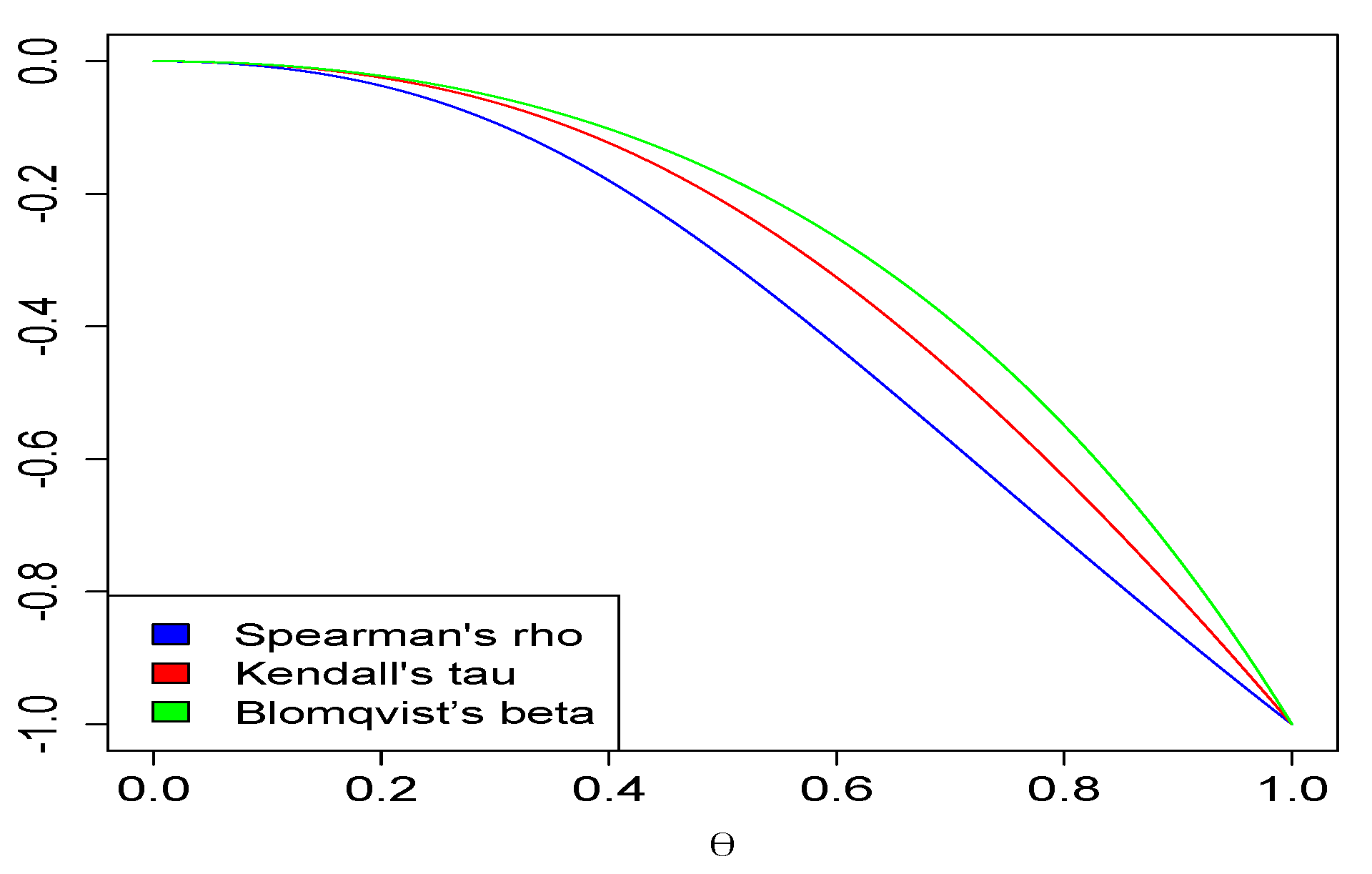
Easy calculations show that the latter is nonincreasing in u for all v, which ensures that RTD ( V | U ) holds. Therefore, Spearman’s rho and Kendall’s tau of C θ described in Proposition 5 are such that ρ θ τ θ 0 . This fact is illustrated in Figure 5.

3.4. Convexity Properties of C θ

In this subsection we address some convexity properties of the copula C θ . We start by recalling the Schur-concavity and the submigrativity properties.
Definition 6.
A bivariate copula C is called Schur concave if for all u, v and γ in [ 0 , 1 ] ,
C ( u , v ) C ( γ u + ( 1 γ ) v , γ v + ( 1 γ ) u ) .
Definition 7.
A bivariate copula C is called submigrative if it is symmetric and satisfies
C ( γ u , v ) C ( u , γ v ) ,
for 0 v u 1 and 0 γ 1 .
Proposition 7.
The copula C θ defined by (3) is Schur concave.
Proof. 
It is clear, after some elementary algebra, that W is Schur concave. The result follows immediately as a consequence of Proposition 9 of Dolati et al. (2014). □
Proposition 8.
The copula C θ defined by (3) is submigrative.
Proof. 
It is easy to show that W is submigrative. We then make use of Proposition 10 of Dolati et al. (2014) to end the proof. □

3.5. Mixed Moment of C θ

In what follows, we derive the expression of the mixed moment corresponding to copula C θ . This result will be of great use in studying the asymptotic behaviour of the estimator of the dependence parameter that will be explored in the next section.
Proposition 9.
If ( U , V ) is a random pair distributed as a copula C θ , then for any nonnegative integers i and j,
E U i V j = α ( i , j , θ ) + β ( i , j , θ ) B i + 1 θ , j + 1 θ ,
where
α ( i , j , θ ) = ( i θ + 1 ) ( j θ + 1 ) i j θ 2 ( i + 1 ) ( j + 1 ) ( i θ + 1 ) ( j θ + 1 )
and
β ( i , j , θ ) = i j ( i θ + 1 ) ( j θ + 1 ) .
Proof. 
Let ( U , V ) be a uniform random pair distributed as a copula C θ . Then one has,
E U i V j = 0 1 0 1 i j u i 1 v j 1 P ( U > u , V > v ) d u d v = 0 1 0 1 i j u i 1 v j 1 ( 1 u v + C θ ( u , v ) ) d u d v = K 1 + K 2 ,
where
K 1 = 0 1 0 1 i j u i 1 v j 1 ( 1 u v ) d u d v = 1 i j ( i + 1 ) ( j + 1 )
and
K 2 = 0 1 0 1 i j u i 1 v j 1 C θ ( u , v ) d u d v = 0 1 0 1 i j u i θ v j θ max ( u θ + v θ 1 , 0 ) d u d v = s 1 + s 2 s 3 .
Straightforward calculations lead to
s 1 = i j 0 1 u i ( 1 u θ ) 1 θ 1 v j θ d v d u = i j j θ + 1 1 i + 1 1 θ B i + 1 θ , j + 1 θ , s 2 = i j 0 1 v j ( 1 v θ ) 1 θ 1 u i θ d u d v = i j i θ + 1 1 j + 1 1 θ B i + 1 θ , j + 1 θ , s 3 = i j 0 1 v j θ ( 1 v θ ) 1 θ 1 u i θ d u d v = i j ( i θ + 1 ) ( j θ + 1 ) 1 i + 1 θ + j + 1 θ 1 B i + 1 θ , j + 1 θ .
Expression (9) can now be derived in a routine manner. □

4. Parameter Estimation

We are now in a position to estimate the parameter of dependence θ by the method of moments and investigate its asymptotic behaviour. Indeed, a consistent estimator of θ can be determined by means of Equation (11).
g ( θ ) = ρ θ = 3 ( 2 θ ) 2 θ 2 4 B 2 θ , 2 θ .
Let ( U 1 , V 1 ) , , ( U n , V n ) be mutually independent copies of ( U , V ) with copula C θ . The estimator θ ^ can be deduced by solving
g ( θ ^ ) = ρ ^ ,
where ρ ^ denotes the sample Spearman’s rho expressed, in terms of ( U 1 , V 1 ) , , ( U n , V n ) , as follows
ρ ^ = 12 n i = 1 n U i V i 3 .
Since the function h is strictly decreasing, the desired estimator is uniquely obtained by
θ ^ = g 1 ( ρ ^ ) .
Note that ρ coincide with the Pearson correlation coefficient of the uniform random vector ( U , V ) distributed as C θ . This means that
g ( θ ) = cor ( U , V ) = 12 cov ( U , V ) .
Consider the covariance sample S 12 expressed in terms of ( U 1 , V 1 ) , , ( U n , V n ) by
S 12 = 1 n 1 i = 1 n U i V i n U ¯ V ¯ ,
where U ¯ and V ¯ denote the sample means of U 1 , , U n and V 1 , , V n , respectively. Clearly, ρ ^ is expressed in terms of S 12 as follows
g ( θ ^ ) = ρ ^ = 12 n 1 n S 12 + U ¯ V ¯ 1 4 .
It is well known (see, e.g., Theorem 8 on p. 52 of Ferguson 1996) that S 12 is a consistent and asymptotically Gaussian estimator of the population covariance cov ( U , V ) , namely
n S 12 cov ( U , V ) N ( 0 , σ ˜ 2 ( θ ) ) as n ,
where σ ˜ 2 ( θ ) ) = var U 1 2 V 1 2 . It follows from (19)–(21) that, as n ,
n g ( θ ^ ) g ( θ ) N ( 0 , σ 2 ( θ ) ) ,
with σ 2 ( θ ) = 144 σ ˜ 2 ( θ ) = 9 var 2 U 1 2 V 1 . A direct application of the Delta Method and Slutsky’s Lemma applied to θ ^ = g 1 ( ρ ^ ) yields the asymptotic law of θ ^ . The following proposition has been proved.
Proposition 10.
For all θ ( 0 , 1 ) , one has
n θ ^ θ N 0 , g ( θ ) 2 σ 2 ( θ ) as n ,
where σ 2 ( θ ) = 9 v a r 2 U 1 2 V 1 for a uniform random vector ( U , V ) with copula C θ .
In order to derive an explicit expression of the asymptotic variance, one can easily see that
σ 2 ( θ ) = 9 E 2 U 1 2 2 V 1 2 E 2 U 1 2 V 1 2 = 144 E U 2 V 2 288 E U V 2 + 216 E U V 144 E U V 2 12 .
Using Proposition 9, one can deduce that
E U V = 1 θ ( 2 θ ) 2 + 1 ( 2 θ ) 2 B 2 θ , 2 θ ,
and
E U V 2 = 6 5 θ θ 2 6 ( 2 θ ) ( 3 θ ) + 2 ( 2 θ ) ( 3 θ ) B 2 θ , 3 θ , E U 2 V 2 = 3 2 θ θ 2 3 ( 3 θ ) 2 + 4 ( 3 θ ) 2 B 3 θ , 3 θ .
This in turn implies that
σ 2 ( θ ) = T 1 ( θ ) B 2 2 θ , 2 θ + T 2 ( θ ) B 2 θ , 2 θ + T 3 ( θ ) B 3 θ , 2 θ + T 4 ( θ ) B 3 θ , 3 θ + T 5 ( θ ) ,
where
T 1 ( θ ) = 144 ( 2 θ ) 4 , T 2 ( θ ) = 72 ( 3 θ 2 8 θ + 8 ) ( 2 θ ) 4 , T 3 ( θ ) = 576 ( 2 θ ) ( 3 θ ) , T 4 ( θ ) = 576 ( 3 θ ) 2 , T 5 ( θ ) = 12 ( θ 6 4 θ 5 θ 4 + 22 θ 3 34 θ 2 + 32 θ 12 ) ( 2 θ ) 4 ( 3 θ ) 2 .
On the other hand, the derivative of g is given by:
g ( θ ) = 12 θ ( 2 θ ) 3 + 24 ( 2 θ ) 3 B 2 θ , 2 θ 48 θ 2 ( 2 θ ) 2 B 1 , 0 2 θ , 2 θ ,
with B 1 , 0 ( x , y ) being the partial derivative of B ( x , y ) defined, for x > 0 and y > 0 , by
B 1 , 0 ( x , y ) = B x ( x , y ) = 0 1 ln ( t ) t x 1 ( 1 t ) y 1 d t = B ( x , y ) ( ψ ( x ) ψ ( x + y ) ) ,
where ψ ( x ) is the Digamma function. This completes the discussion on the asymptotic variance.

5. Simulation Study

In the following, we will examine the performance of θ ^ , the estimator of the dependence parameter θ established previously, and then provide an asymptotic confidence interval for θ . To do this, we will consider different values of Spearman’s rho for the copula C θ . Theoretical values of θ can thereby be obtained by solving
g ( θ ) = ρ θ = 3 ( 2 θ ) 2 θ 2 4 B 2 θ , 2 θ .
Let ( U 1 , V 1 ) , , ( U n , V n ) be mutually independent copies of the vector of unit uniform random variables ( U , V ) with copula C θ . The estimator of the dependence parameter θ is then uniquely obtained by solving θ ^ = h 1 ( ρ ^ ) , where ρ ^ denotes the sample version of Spearman’s rho. Different sample sizes, n, are considered with 500 replications of each possible scenario.
The results of the estimator θ ^ , bias, mean squared error (MSE) and 95 % asymptotic confidence interval estimations of θ are reported in the next tables. In each of the scenarios under investigation, simulations demonstrate that θ ^ provides a good estimator for the dependence parameter θ . Not surprisingly, the effectiveness of our estimator θ ^ increases as n becomes larger: bias and MSE of θ ^ decrease while the confidence intervals become narrower. This can be seen upon looking at the behaviour of the estimator θ ^ in three different scenarios, weak, moderate and strong dependence in Table 1.

6. Real Data Study

This section is devoted to analyzing a data set based on the proposed copula and estimation methodology described earlier. In our study, “airquality”, which refers to a data set on the daily quality of air, will be considered. The data collected are based on 153 successive days in the New York Metropolitan Area. The two variables explored here are average wind speed (in miles per hour) and mean ozone level (in parts per billion). See (Chambers et al. 1983, Appendix, Data set 2) for a thorough description of the data. This data set is also available in the R package “datasets”.
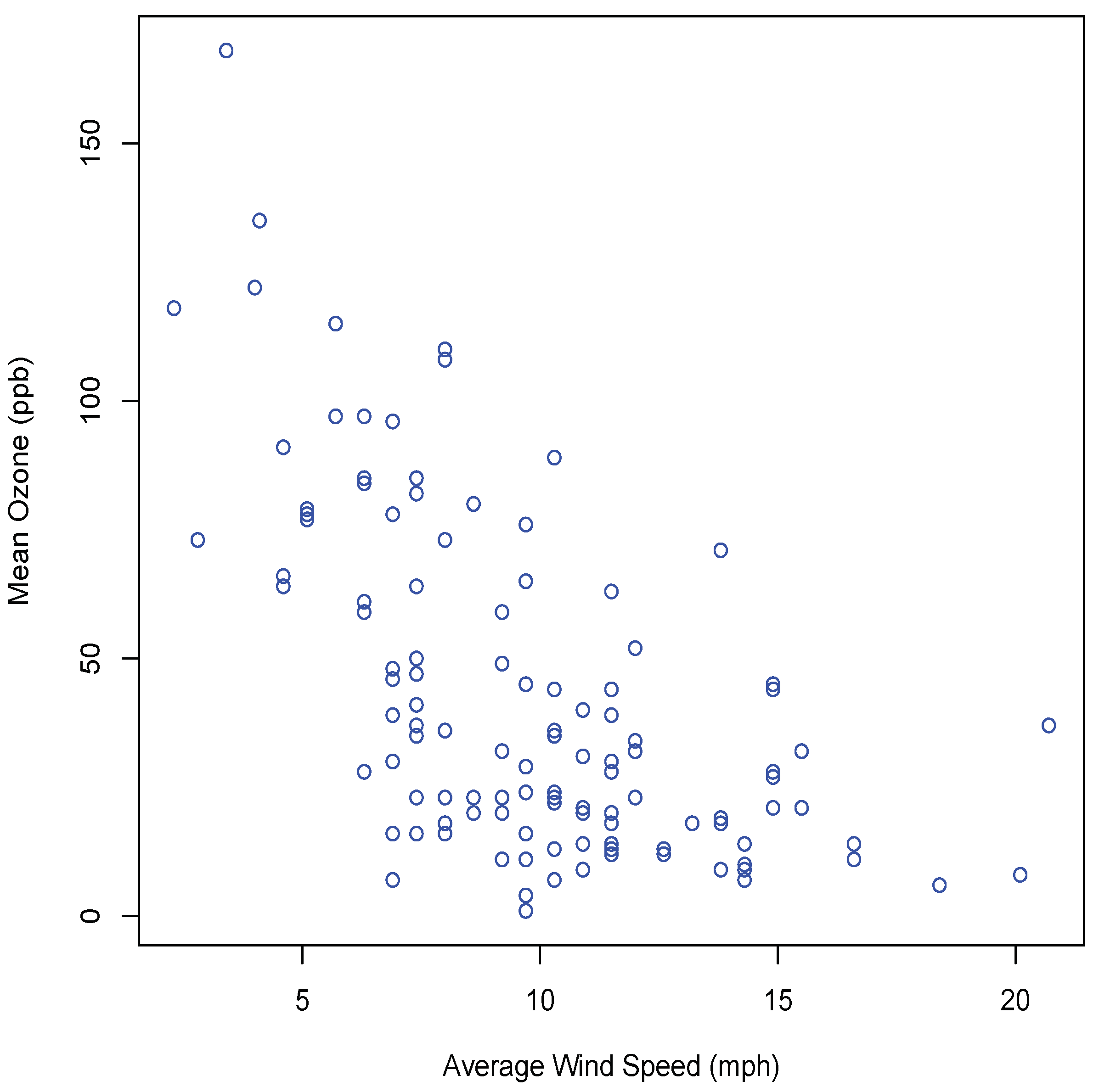
In this analysis, 116 observations are inspected, ignoring the missing values. The following scatter plot (Figure 6) indicates a negative dependence between average wind speed and mean ozone level which is supported by negative values of Spearman’s rho and Kendall’s tau coefficients, 0.59 and 0.43, respectively. To analyze this phenomenon, we fit the proposed copula using the method of moments. To do this, we propose five models, commonly used in the field of engendering and environmental science: Weibull, lognormal Gamma, Beta four parameters (Beta4) and Generalized Extreme Value distribution (GEVD) for modeling average wind speed and mean ozone level. Based on the Akaike information criterion (AIC) and the Bayesian information criterion (BIC), as shown in Table 2 and Table 3, we find that the Gamma distribution fits both marginals better than the other proposed models.
Using the bootstrap technique based on Kolmogorov–Smirnov (KS) and Anderson–Darling (AD) goodness-of-fit (GOF) tests, Table 4 demonstrate that Gamma distribution is a good fit for both marginals. The maximum likelihood estimates (MLEs) of the parameters are shown in the same table.
The estimate of the dependence parameter of the proposed copula is obtained by solving θ ^ = g 1 ( ρ ) for ρ ^ = 0.59 (see (18)). It is found to be θ ^ = 0.711 . Now, we evaluate the GOF tests of the proposed copula C θ , based on Kolmogorov–Smirnov and Cramér–von Mises statistics using the bootstrap algorithm proposed by Genest et al. (2009). Table 5 shows that our proposed model fits the data set reasonably well.

7. Conclusions

We have introduced a new negatively quadrant bivariate family of copulas by means of the counter-monotonic shock method. The properties of this family were derived, and a moment-based estimator for the parameter of dependence was investigated. The usefulness of the copula was illustrated through simulations and a real case study dealing with the daily air quality measurements for the New York Metropolitan Area. We argue that this new approach-based copula is easy to simulate and interpret and will be a great addition to the theory of copulas. A generalization of this family will be explored, in a forthcoming paper, by examining a model with two dependence parameters, θ 1 and θ 2 , to allow for more flexible modeling. Another possible direction of future research could be a a general model describing both positive and negative dependence.

Author Contributions

F.E.K., R.B., N.S. and M.M. contributed equally to this work. All authors have read and agreed to the published version of the manuscript.

Funding

The work of the first three authors is funded by Zayed University. The work of the fourth author is funded by the Natural Sciences and Engineering Research Council of Canada No. 06536-2018.

Acknowledgments

The authors would like to thank the three anonymous referees for their useful comments and suggestions, which helped to improve the manuscript.

Conflicts of Interest

The authors declare no conflict of interest.

References

  1. Almongy, Hisham Mohamed, Ehab Mohamed Almetwally, and Amaal Elsayed Mubarak. 2021. Marshall–Olkin Alpha Power Lomax Distribution: Estimation Methods, Applications on Physics and Economics. Pakistan Journal of Statistics and Operation Research 17: 137–53. [Google Scholar] [CrossRef]
  2. Bentoumi, Rachid, Farid El Ktaibi, and Mhamed Mesfioui. 2021. A New Family of Bivariate Exponential Distributions with Negative Dependence Based on Counter-Monotonic Shock Method. Entropy 23: 548. [Google Scholar] [CrossRef] [PubMed]
  3. Cuadras, Carles M., and Joan Augé. 1981. A continuous general multivariate distribution and its properties. Communications in Statistics-Theory and Methods 10: 339–53. [Google Scholar] [CrossRef]
  4. Chambers, John M., William S. Cleveland, Beat Kleiner, and Paul A. Tukey. 1983. Graphical Methods for Data Analysis. London: Taylor & Francis/CRC. [Google Scholar]
  5. Capéraà, Philippe, and Christian Genest. 1993. Spearman’s is larger than Kendall’s for positively dependent random variables. Journal of Nonparametric Statistics 2: 183–94. [Google Scholar] [CrossRef]
  6. Dolati, Ali, Soheyla Mohseni, and Manuel Úbeda-Flores. 2014. Some results on a transformation of copulas and quasi-copulas. Information Sciences 257: 176–82. [Google Scholar] [CrossRef]
  7. Durante, Fabrizio. 2009. Construction of non-exchangeable bivariate distribution functions. Statistical Papers 50: 383–91. [Google Scholar] [CrossRef]
  8. El-Morshedy, Mahmoud, Ziyad Ali Alhussain, Doaa Atta, Ehab M. Almetwally, and Mohammed. S. Eliwa. 2020. Bivariate Burr X Generator of Distributions: Properties and Estimation Methods with Applications to Complete and Type-II Censored Samples. Mathematics 14: 264. [Google Scholar] [CrossRef] [Green Version]
  9. Eliwa, Mohammed. S., and Mahmoud El-Morshedy. 2020. Bivariate odd Weibull-G family of distributions: Properties, Bayesian and non-Bayesian estimation with bootstrap confidence intervals and application. Journal of Taibah University for Science 8: 331–45. [Google Scholar] [CrossRef] [Green Version]
  10. Ferguson, Thomas S. 1996. A Course in Large Sample Theory. London: Chapman & Hall/CRC. [Google Scholar]
  11. Fredricks, Gregory A., and Roger B. Nelsen. 2007. On the Relationship between Spearman’s Rho and Kendall’s Tau for Pairs of Continuous Random Variables. Journal of Statistical Planning and Inference 137: 2143–50. [Google Scholar] [CrossRef]
  12. Genest, Christian, Bruno Rémillard, and David Beaudoin. 2009. Goodness-of-fit tests for copulas: A review and a power study. Insurance: Mathematics and Economics 44: 199–213. [Google Scholar] [CrossRef]
  13. Genest, Christian, Mhamed Mesfioui, and Juliana Schulz. 2018. A new bivariate Poisson common shock model covering all possible degrees of dependence. Statistics and Probability Letters 140: 202–9. [Google Scholar] [CrossRef]
  14. Haj Ahmad, Hanan, and Ehab M. Almetwally. 2020. Marshall–Olkin Generalized Pareto Distribution: Bayesian and Non Bayesian Estimation. Pakistan Journal of Statistics and Operation Research 16: 21–33. [Google Scholar] [CrossRef] [Green Version]
  15. Khoudraji, Abdelhaq. 1995. Contributions à l’étude des Copules et à la Modélisation des Valeurs Extrêmes Bivariées. Ph.D. thesis, Université de Laval, Québec, QC, Canada. [Google Scholar]
  16. Kole, Erik, Kees Koedijk, and Marno Verbeek. 2007. Selecting copulas for risk management. Journal of Banking & Finance 31: 2405–23. [Google Scholar]
  17. Lehmann, Erich Leo. 1966. Some concepts of dependence. The Annals of Mathematical Statistics 37: 1137–53. [Google Scholar] [CrossRef]
  18. Liebscher, Eckhard. 2008. Construction of asymmetric multivariate copulas. Journal of Multivariate Analysis 99: 2234–50. [Google Scholar] [CrossRef] [Green Version]
  19. Marshall, Albert W., and Ingram Olkin. 1967. A multivariate exponential distribution. Journal of the American Statistical Association 62: 30–44. [Google Scholar] [CrossRef]
  20. Mesfioui, Mhamed, and Abdelouahid Tajar. 2005. On the properties of some nonparametric concordance measures in the discrete case. Nonparametric Statistics 17: 541–54. [Google Scholar] [CrossRef]
  21. Nelsen, Roger B. 2006. An Introduction to Copulas. New York: Springer. [Google Scholar]
  22. Ruiz-Rivas, Carmen, and Carles M. Cuadras. 1988. Inference properties of a one-parameter curved exponential family of distributions with given marginals. Journal of Multivariate Analysis 27: 447–56. [Google Scholar] [CrossRef]
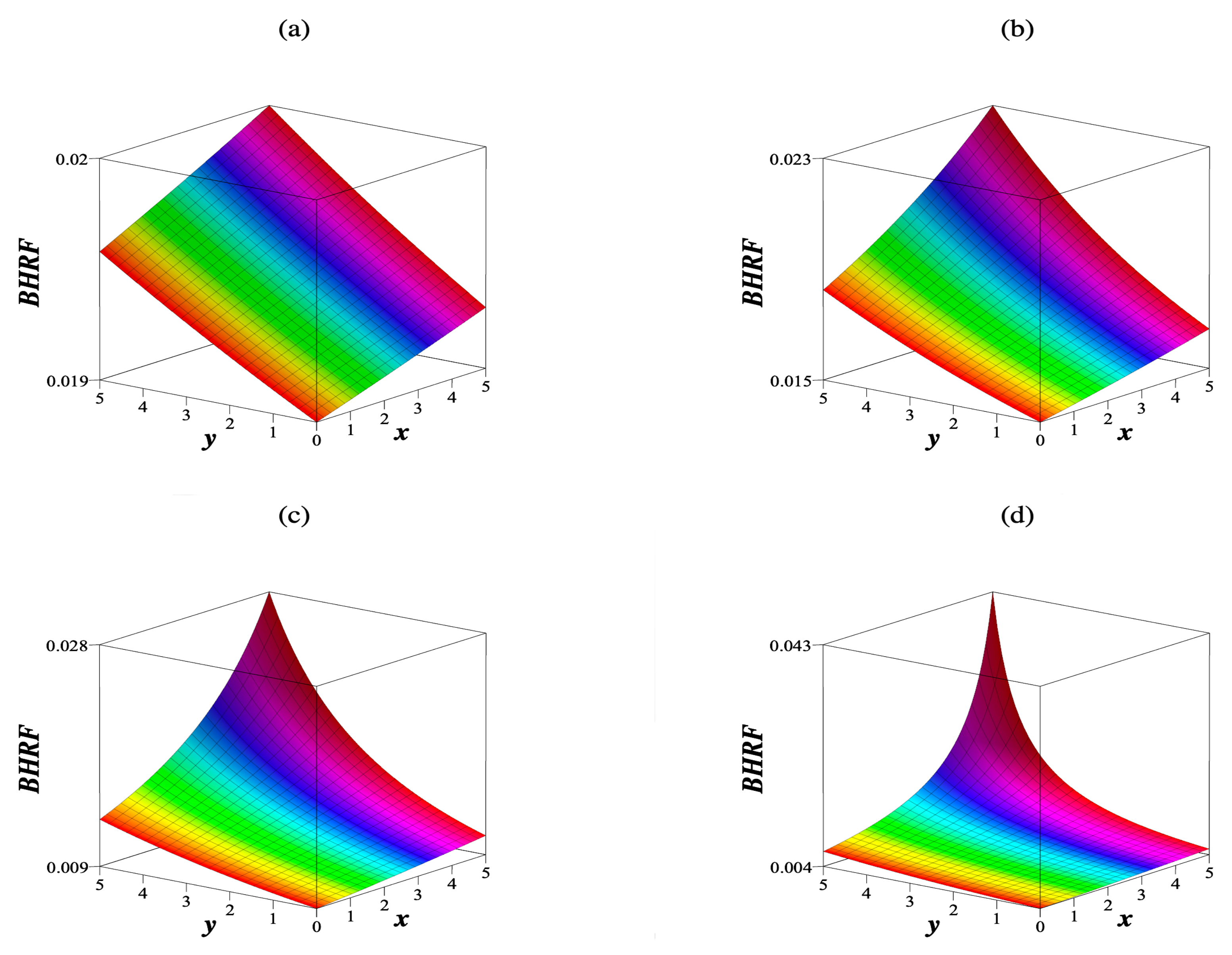
Figure 1. Bivariate hazard rate functions for ( λ 1 , λ 2 ) = ( 0.1 , 0.2 ) and different values of θ : (a) θ = 0.2 , (b) θ = 0.5 , (c) θ = 0.75 and (d) θ = 0.9 .
Risks 10 00202 g001
Figure 2. Scatterplots for C θ .
Risks 10 00202 g002
Figure 3. Copulas C θ for (a) θ = 0.2 , (b) θ = 0.5 , (c) θ = 0.75 and (d) θ = 0.9 .
Risks 10 00202 g003
Figure 4. Copula density for (a) θ = 0.2 , (b) θ = 0.5 , (c) θ = 0.75 and (d) θ = 0.9 .
Risks 10 00202 g004
Figure 5. Graph of Spearman’s rho, Kendall’s tau and Blomqvist’s beta.
Risks 10 00202 g005
Figure 6. Scatter plot of average wind speed versus mean ozone.
Risks 10 00202 g006
Table 1. Moment-based estimation for θ .
n θ ^ Bias( θ ^ )MSE( θ ^ )95% CI
ρ = 0.1 θ = 0.3098 50 0.4717 0.1619 0.0262 ( 0.2202 , 0.7232 )
100 0.4308 0.1209 0.0146 ( 0.2328 , 0.6287 )
200 0.3798 0.0699 0.0049 ( 0.2400 , 0.5195 )
300 0.3563 0.0465 0.0022 ( 0.2407 , 0.4720 )
400 0.3450 0.0352 0.0012 ( 0.2492 , 0.4408 )
ρ = 0.2 θ = 0.4190 50 0.5120 0.0930 0.0087 ( 0.3031 , 0.7209 )
100 0.4653 0.0463 0.0021 ( 0.3146 , 0.6158 )
200 0.4385 0.0195 0.0004 ( 0.3194 , 0.5575 )
300 0.4214 0.0024 5 × 10 6 ( 0.3201 , 0.5227 )
400 0.4210 0.0020 4 × 10 6 ( 0.3332 , 0.5088 )
ρ = 0.3 θ = 0.5038 50 0.5508 0.0470 0.0022 ( 0.3509 , 0.7507 )
100 0.5173 0.0136 0.0002 ( 0.3707 , 0.6640 )
200 0.5055 0.0017 2 × 10 6 ( 0.4000 , 0.6107 )
300 0.5020 0.0017 3 × 10 6 ( 0.4155 , 0.5885 )
400 0.5048 0.0010 10 6 ( 0.4289 , 0.5807 )
ρ = 0.4 θ = 0.5788 50 0.5972 0.0184 0.0003 ( 0.4042 , 0.7902 )
100 0.5761 0.0028 7 × 10 6 ( 0.4377 , 0.7144 )
200 0.5765 0.0023 5 × 10 6 ( 0.4787 , 0.6743 )
300 0.5770 0.0018 3 × 10 6 ( 0.4972 , 0.6569 )
400 0.5791 0.0003 9 × 10 8 ( 0.5101 , 0.6481 )
ρ = 0.5 θ = 0.6494 50 0.6460 0.0034 10 5 ( 0.4571 , 0.8349 )
100 0.6508 0.0014 2 × 10 6 ( 0.5174 , 0.7842 )
200 0.6491 0.0003 10 7 ( 0.5547 , 0.7434 )
300 0.6491 0.0003 8 × 10 8 ( 0.5721 , 0.7261 )
400 0.6496 0.0002 6 × 10 8 ( 0.5816 , 0.7176 )
ρ = 0.6 θ = 0.7181 50 0.7087 0.0093 8 × 10 5 ( 0.5220 , 0.8954 )
100 0.7121 0.0059 4 × 10 5 ( 0.5801 , 0.8441 )
200 0.7159 0.0021 5 × 10 6 0.6226 , 0.8092 )
300 0.7188 0.0007 5 × 10 7 ( 0.6246 , 0.8112 )
400 0.7176 0.0004 2 × 10 7 ( 0.6426 , 0.7926 )
ρ = 0.7 θ = 0.7864 50 0.7529 0.0336 0.0011 ( 0.5664 , 0.9393 )
100 0.7758 0.0106 0.0001 ( 0.6439 , 0.9078 )
200 0.7879 0.0015 2 × 10 6 ( 0.6946 , 0.8812 )
300 0.7861 0.0004 10 7 ( 0.7099 , 0.8623 )
400 0.7866 0.0002 3 × 10 8 ( 0.7104 , 0.8628 )
ρ = 0.8 θ = 0.8556 50 0.8101 0.0455 0.0021 ( 0.6232 , 0.9971 )
100 0.8337 0.0219 0.0005 ( 0.7013 , 0.9661 )
200 0.8540 0.0016 3 × 10 6 ( 0.7603 , 0.9477 )
300 0.8542 0.0015 2 × 10 6 ( 0.7777 , 0.9307 )
400 0.8565 0.0008 6 × 10 7 ( 0.7902 , 0.9227 )
ρ = 0.9 θ = 0.9265 50 0.8654 0.0611 0.0037 ( 0.6779 , 1 )
100 0.8951 0.0314 0.0010 ( 0.7624 , 1 )
200 0.9099 0.0166 0.0003 ( 0.8161 , 1 )
300 0.9187 0.0078 6 × 10 5 ( 0.8421 , 0.9953 )
400 0.9223 0.0042 2 × 10 5 ( 0.8560 , 0.9887 )
Table 2. AIC and BIC criteria for average wind.
WeibullLognormalGammaBeta4GEVD
AIC625.408631.862624.490626.947624.942
BIC630.916637.370629.997637.961633.203
Table 3. AIC and BIC criteria for mean ozone level.
WeibullLognormalGammaBeta4GEVD
AIC1089.2211091.7661087.0751090.8031093.552
BIC1094.7281097.2731092.5831101.8171101.813
Table 4. KS and AD goodness-of-fit tests for Gamma distribution and MLE parameters.
Average WindMean Ozone Level
KSADKSAD
Test statistic0.0730.4810.0800.738
p-value0.5370.7660.4200.527
Shape7.171.70
Scale1.37524.770
Table 5. Goodness-of-fit test for C θ .
KSCramér–von Mises
Test statistic T n = 0.078 S n = 0.120
p-value0.5840.219
Publisher’s Note: MDPI stays neutral with regard to jurisdictional claims in published maps and institutional affiliations.