
A Comparative Analysis of Optimization Algorithms for Gastrointestinal Abnormalities Recognition and Classification Based on Ensemble XcepNet23 and ResNet18 Features

 , ,
, ,  ,
,  and
and 
Abstract
1. Introduction
- ▪
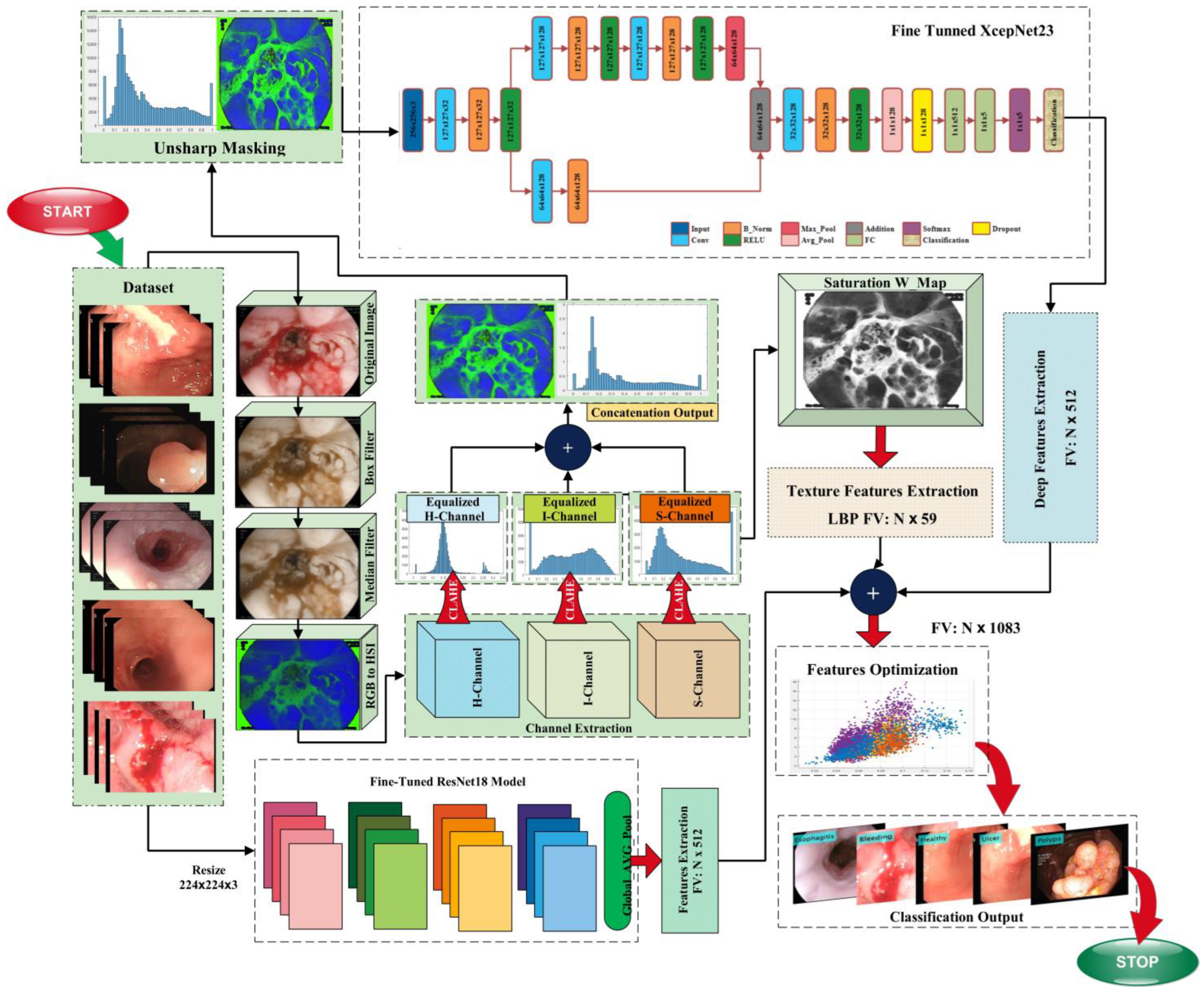
- Contrast enhancement is one of the main contributions of this research work. In the pre-processing step, hybrid contrast enhancement methods are used to improve lesion contrast. The major steps performed in the pre-processing phase are 3D-box filtering, 3D-median filtering, HSI color transformation, and channels extraction. Contrast Limited Adaptive Histogram Equalization (CLAHE) is employed on the extracted channels and gives the output H_CLAHE, S-CLAHE, and I_CLAHE; in the next step, the saturation Weight-Map is applied on the S_CLAHE. In the last step of the pre-processing phase, un-sharp masking is employed on the concatenated output.
- ▪
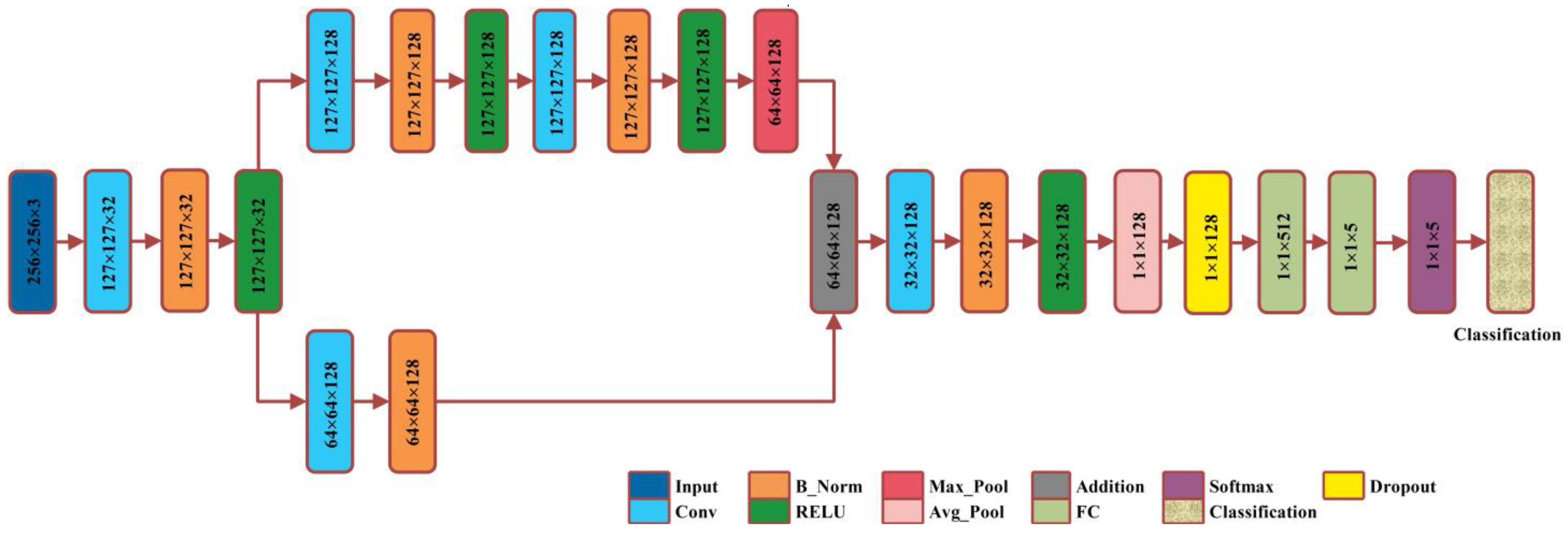
- A CNN model is designed from scratch with 23 layers, named XcepNet23. The proposed CNN model is pretrained on the CIPHER-100 dataset. Features engineering is performed on the extracted deep features.
- ▪
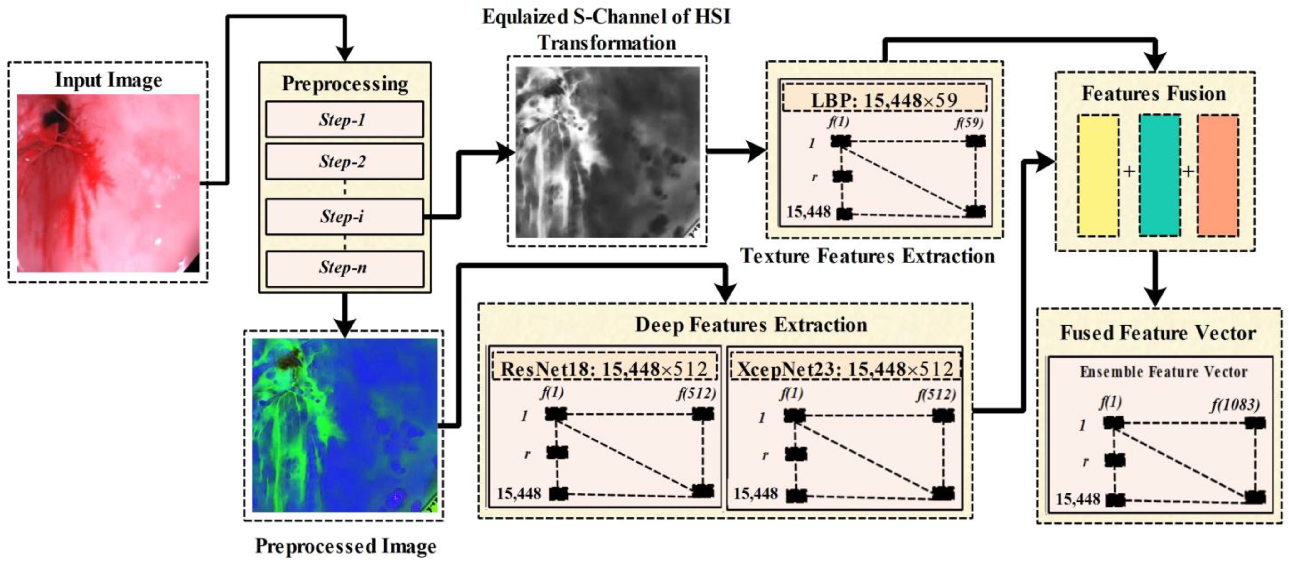
- A hybrid features engineering methodology is proposed. Features vectors are obtained using the fine-tuned ResNet18 model, the proposed XcepNet23, and LBP features. The strong feature vector is created by combining the texture features and the extracted features from the two CNN models. The BDA, MFO, and PSO algorithms are used to optimize the fused feature vector.
2. Related Work
3. Proposed Methodology
3.1. Preprocessing
3.1.1. Data Augmentation
3.1.2. D-Box Filtering
3.1.3. D-Median Filtering
3.1.4. HSI Color Transformation
3.1.5. Contrast Limited Adaptive Histogram Equalization
3.2. Feature Extraction
3.2.1. Local Binary Pattern
3.2.2. Deep Learning Features
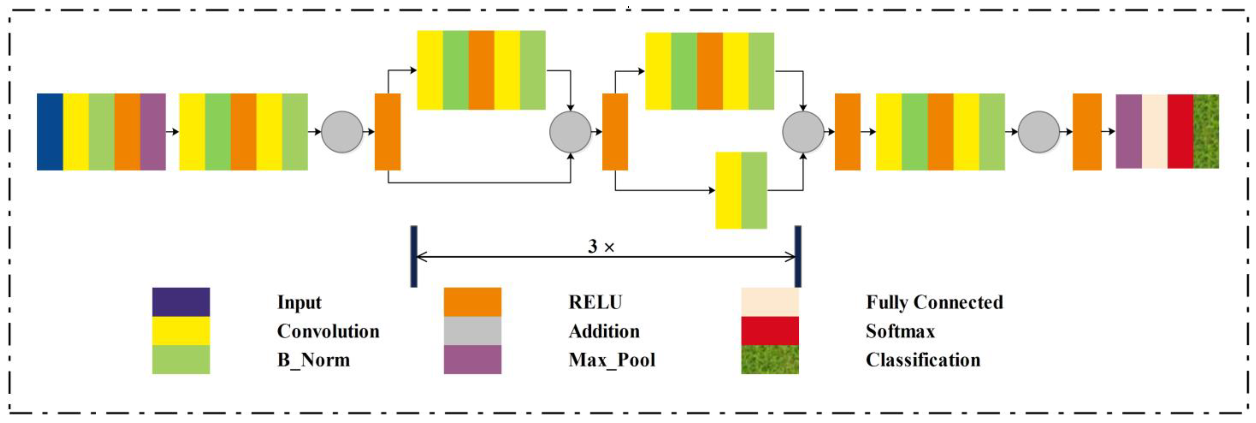
ResNet18
Proposed XcepNet23
3.2.3. Features Optimization
4. Experimental Results and Analysis
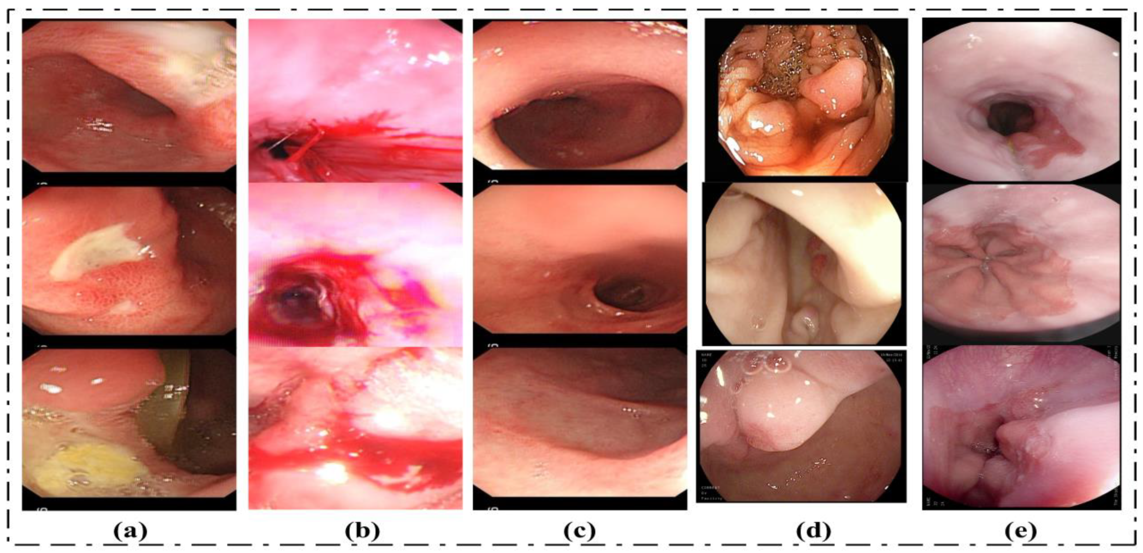
4.1. Dataset
4.2. Performance Measures
4.3. Results
4.3.1. Experiment 1: Results on the Feature Vector
4.3.2. Experiment 2: Results on the Feature Vector
4.3.3. Experiment 3: Results on the Feature Vector
4.3.4. Experiment 4: Results on the Feature Vector
5. Discussion and Comparison with Existing Methods
6. Conclusions
Author Contributions
Funding
Institutional Review Board Statement
Informed Consent Statement
Data Availability Statement
Acknowledgments
Conflicts of Interest
References
- Sharif, M.; Khan, M.A.; Rashid, M.; Yasmin, M.; Afza, F.; Tanik, U.J. Deep CNN and geometric features-based gastrointestinal tract diseases detection and classification from wireless capsule endoscopy images. J. Exp. Theor. Artif. Intell. 2019, 33, 577–599. [Google Scholar] [CrossRef]
- Mohammad, F.; Al-Razgan, M. Deep Feature Fusion and Optimization-Based Approach for Stomach Disease Classification. Sensors 2022, 22, 2801. [Google Scholar] [CrossRef]
- Khan, M.A.; Kadry, S.; Alhaisoni, M.; Nam, Y.; Zhang, Y.-D.; Rajinikanth, V.; Sarfaraz, M.S. Computer-Aided Gastrointestinal Diseases Analysis from Wireless Capsule Endoscopy: A Framework of Best Features Selection. IEEE Access 2020, 8, 132850–132859. [Google Scholar] [CrossRef]
- Kourie, H.R.; Tabchi, S.; Ghosn, M. Checkpoint inhibitors in gastrointestinal cancers: Expectations and reality. World J. Gastroenterol. 2017, 23, 3017–3021. [Google Scholar] [CrossRef] [PubMed]
- Long, J.; Lin, J.; Wang, A.; Wu, L.; Zheng, Y.; Yang, X.; Wan, X.; Xu, H.; Chen, S.; Zhao, H. PD-1/PD-L blockade in gastrointestinal cancers: Lessons learned and the road toward precision immunotherapy. J. Hematol. Oncol. 2017, 10, 146. [Google Scholar] [CrossRef] [PubMed]
- Umar, S.B.; Fleischer, D.E. Esophageal cancer: Epidemiology, pathogenesis and prevention. Nat. Clin. Pract. Gastroenterol. Hepatol. 2008, 5, 517–526. [Google Scholar] [CrossRef]
- Pennathur, A.; Gibson, M.K.; Jobe, B.A.; Luketich, J.D. Oesophageal carcinoma. Lancet 2013, 381, 400–412. [Google Scholar] [CrossRef] [PubMed]
- Bray, F.; Ferlay, J.; Soerjomataram, I.; Siegel, R.L.; Torre, L.A.; Jemal, A. Global cancer statistics 2018: GLOBOCAN estimates of incidence and mortality worldwide for 36 cancers in 185 countries. CA Cancer J. Clin. 2018, 68, 394–424. [Google Scholar] [CrossRef] [PubMed]
- Sivakumar, P.; Kumar, B.M. A novel method to detect bleeding frame and region in wireless capsule endoscopy video. Clust. Comput. 2019, 22, 12219–12225. [Google Scholar] [CrossRef]
- Amin, J.; Sharif, M.; Yasmin, M.; Fernandes, S.L. A distinctive approach in brain tumor detection and classification using MRI. Pattern Recognit. Lett. 2020, 139, 118–127. [Google Scholar] [CrossRef]
- Amin, J.; Sharif, M.; Yasmin, M.; Ali, H.; Fernandes, S.L. A method for the detection and classification of diabetic retinopathy using structural predictors of bright lesions. J. Comput. Sci. 2017, 19, 153–164. [Google Scholar] [CrossRef]
- Liaqat, A.; Khan, M.A.; Shah, J.H.; Sharif, M.; Yasmin, M.; Fernandes, S.L. Automated ulcer and bleeding classification from wce images using multiple features fusion and selection. J. Mech. Med. Biol. 2018, 18, 1850038. [Google Scholar] [CrossRef]
- Lee, N.M.; Eisen, G.M. 10 years of capsule endoscopy: An update. Expert Rev. Gastroenterol. Hepatol. 2010, 4, 503–512. [Google Scholar] [CrossRef] [PubMed]
- Saeed, T.; Loo, C.K.; Kassim, M.S.S. Ensembles of Deep Learning Framework for Stomach Abnormalities Classification. Comput. Mater. Contin. 2022, 70, 4357–4372. [Google Scholar] [CrossRef]
- Rajinikanth, V.; Satapathy, S.C.; Fernandes, S.L.; Nachiappan, S. Entropy based segmentation of tumor from brain MR images—A study with teaching learning based optimization. Pattern Recognit. Lett. 2017, 94, 87–95. [Google Scholar] [CrossRef]
- Rajinikanth, V.; Fernandes, S.L.; Bhushan, B.; Harisha; Sunder, N.R. Segmentation and analysis of brain tumor using Tsallis entropy and regularised level set. In Proceedings of the 2nd International Conference on Micro-Electronics, Electromagnetics and Telecommunications; Springer: Berlin/Heidelberg, Germany, 2018; pp. 313–321. [Google Scholar]
- Bokhari, S.T.F.; Sharif, M.; Yasmin, M.; Fernandes, S.L. Fundus Image Segmentation and Feature Extraction for the Detection of Glaucoma: A New Approach. Curr. Med. Imaging Former. Curr. Med. Imaging Rev. 2018, 14, 77–87. [Google Scholar] [CrossRef]
- Naqi, S.; Sharif, M.; Yasmin, M.; Fernandes, S.L. Lung Nodule Detection Using Polygon Approximation and Hybrid Features from CT Images. Curr. Med. Imaging Former. Curr. Med. Imaging Rev. 2018, 14, 108–117. [Google Scholar] [CrossRef]
- Naz, J.; Khan, M.A.; Alhaisoni, M.; Song, O.-Y.; Tariq, U.; Kadry, S. Segmentation and Classification of Stomach Abnormalities Using Deep Learning. Comput. Mater. Contin. 2021, 69, 607–625. [Google Scholar] [CrossRef]
- Nida, N.; Sharif, M.; Khan, M.U.G.; Yasmin, M.; Fernandes, S.L. A framework for automatic colorization of medical imaging. IIOAB J. 2016, 7, 202–209. [Google Scholar]
- Suman, S.; Hussin, F.A.; Malik, A.S.; Walter, N.; Goh, K.L.; Hilmi, I. Image enhancement using geometric mean filter and gamma correction for WCE images. In Proceedings of the International Conference on Neural Information Processing, Kuching, Malaysia, 3–6 November 2014; Springer: Berlin/Heidelberg, Germany; pp. 276–283. [Google Scholar]
- Rajinikanth, V.; Madhavaraja, N.; Satapathy, S.C.; Fernandes, S.L. Otsu’s multi-thresholding and active contour snake model to segment dermoscopy images. J. Med. Imaging Health Inform. 2017, 7, 1837–1840. [Google Scholar] [CrossRef]
- Lee, Y.-G.; Yoon, G. Real-time image analysis of capsule endoscopy for bleeding discrimination in embedded system platform. Int. J. Biomed. Biol. Eng. 2011, 5, 583–587. [Google Scholar]
- Yuan, Y.; Li, B.; Meng, M.Q.-H. WCE Abnormality Detection Based on Saliency and Adaptive Locality-Constrained Linear Coding. IEEE Trans. Autom. Sci. Eng. 2016, 14, 149–159. [Google Scholar] [CrossRef]
- Fu, Y.; Zhang, W.; Mandal, M.; Meng, M.Q.-H. Computer-aided bleeding detection in WCE video. IEEE J. Biomed. Health Inform. 2013, 18, 636–642. [Google Scholar] [CrossRef]
- Mathew, M.; Gopi, V.P. Transform based bleeding detection technique for endoscopic images. In Proceedings of the 2015 2nd International Conference on Electronics and Communication Systems (ICECS), Coimbatore, India, 26–27 February 2015; IEEE: Piscateville, NJ, USA; pp. 1730–1734. [Google Scholar]
- Yuan, Y.; Meng, M.Q.-H. Polyp classification based on bag of features and saliency in wireless capsule endoscopy. In Proceedings of the 2014 IEEE International Conference on Robotics and Automation (ICRA), Hong Kong, China, 31 May–7 June 2014; IEEE: Piscateville, NJ, USA; pp. 3930–3935. [Google Scholar]
- Ghosh, T.; Bashar, S.K.; Alam, S.; Wahid, K.; Fattah, S.A. A statistical feature based novel method to detect bleeding in wireless capsule endoscopy images. In Proceedings of the 2014 International Conference on Informatics, Electronics & Vision (ICIEV), Dhaka, Bangladesh, 23–24 May 2014; IEEE: Piscateville, NJ, USA; pp. 1–4. [Google Scholar]
- Yuan, Y.; Meng, M.Q.-H. Deep learning for polyp recognition in wireless capsule endoscopy images. Med. Phys. 2017, 44, 1379–1389. [Google Scholar] [CrossRef]
- Yuan, Y.; Wang, J.; Li, B.; Meng, M.Q.-H. Saliency Based Ulcer Detection for Wireless Capsule Endoscopy Diagnosis. IEEE Trans. Med. Imaging 2015, 34, 2046–2057. [Google Scholar] [CrossRef]
- Suman, S.; Hussin, F.A.; Malik, A.S.; Ho, S.H.; Hilmi, I.; Leow, A.H.-R.; Goh, K.-L. Feature Selection and Classification of Ulcerated Lesions Using Statistical Analysis for WCE Images. Appl. Sci. 2017, 7, 1097. [Google Scholar] [CrossRef]
- Sutton, R.T.; Zaïane, O.R.; Goebel, R.; Baumgart, D.C. Artificial intelligence enabled automated diagnosis and grading of ulcerative colitis endoscopy images. Sci. Rep. 2022, 12, 2748. [Google Scholar] [CrossRef] [PubMed]
- Nayyar, Z.; Khan, M.A.; Alhussein, M.; Nazir, M.; Aurangzeb, K.; Nam, Y.; Kadry, S.; Haider, S.I. Gastric Tract Disease Recognition Using Optimized Deep Learning Features. Comput. Mater. Contin. 2021, 68, 2041–2056. [Google Scholar] [CrossRef]
- Zhang, G.; Pan, J.; Xing, C. Computer-aided diagnosis of digestive tract tumor based on deep learning for medical images. Netw. Model. Anal. Health Inform. Bioinform. 2022, 11, 8. [Google Scholar] [CrossRef]
- Naz, J.; Sharif, M.; Raza, M.; Shah, J.H.; Yasmin, M.; Kadry, S.; Vimal, S. Recognizing Gastrointestinal Malignancies on WCE and CCE Images by an Ensemble of Deep and Handcrafted Features with Entropy and PCA Based Features Optimization. Neural Process. Lett. 2021, 55, 115–140. [Google Scholar] [CrossRef]
- Liu, Y. Noise reduction by vector median filtering. Geophysics 2013, 78, V79–V87. [Google Scholar] [CrossRef]
- Chien, C.-L.; Tseng, D.-C. Color image enhancement with exact HSI color model. Int. J. Innov. Comput. Inf. Control. 2011, 7, 6691–6710. [Google Scholar]
- Ibraheem, N.A.; Hasan, M.M.; Khan, R.Z.; Mishra, P.K. Understanding color models: A review. ARPN J. Sci. Technol. 2012, 2, 265–275. [Google Scholar]
- Saalfeld, S. CLAHE (Contrast Limited Adaptive Histogram Equalization). 2009. Available online: https://imagej.nih.gov/ij/plugins/clahe/index.html (accessed on 8 June 2023).
- Ojala, T.; Pietikainen, M.; Harwood, D. Performance evaluation of texture measures with classification based on Kullback discrimination of distributions. In Proceedings of the 12th International Conference on Pattern Recognition, Jerusalem, Israel, 9–13 October 1994; IEEE Computer Society Press: Piscataway, NJ, USA, 1994; pp. 582–585. [Google Scholar]
- He, K.; Zhang, X.; Ren, S.; Sun, J. Deep residual learning for image recognition. In Proceedings of the IEEE Conference on Computer Vision and Pattern Recognition, Las Vegas, NV, USA, 27–30 June 2016; pp. 770–778. [Google Scholar]
- Khan, M.A.; Muhammad, K.; Wang, S.H.; Alsubai, S.; Binbusayyis, A.; Alqahtani, A.; Majumdar, A.; Thinnukool, O. Gastrointestinal diseases recognition: A framework of deep neural network and improved moth-crow optimization with DCCA fusion. Hum.-Cent. Comput. Inf. Sci. 2022, 12, 25. [Google Scholar]
- Khan, M.A.; Majid, A.; Hussain, N.; Alhaisoni, M.; Zhang, Y.-D.; Kadry, S.; Nam, Y. Multiclass Stomach Diseases Classification Using Deep Learning Features Optimization. Comput. Mater. Contin. 2021, 67, 3381–3399. [Google Scholar] [CrossRef]
- Khan, M.A.; Khan, M.A.; Ahmed, F.; Mittal, M.; Goyal, L.M.; Hemanth, D.J.; Satapathy, S.C. Gastrointestinal diseases segmentation and classification based on duo-deep architectures. Pattern Recognit. Lett. 2020, 131, 193–204. [Google Scholar] [CrossRef]
- Too, J.; Mirjalili, S. A Hyper Learning Binary Dragonfly Algorithm for Feature Selection: A COVID-19 Case Study. Knowl.-Based Syst. 2021, 212, 106553. [Google Scholar] [CrossRef]
- Mirjalili, S. Dragonfly algorithm: A new meta-heuristic optimization technique for solving single-objective, discrete, and multi-objective problems. Neural Comput. Appl. 2016, 27, 1053–1073. [Google Scholar] [CrossRef]
- Mirjalili, S. Moth-flame optimization algorithm: A novel nature-inspired heuristic paradigm. Knowl. Based Syst. 2015, 89, 228–249. [Google Scholar] [CrossRef]
- Eberhart, R.; Kennedy, J. Particle swarm optimization. In Proceedings of the IEEE International Conference on Neural Networks, Perth, Australia, 27 November–1 December 1995; Volume 4, pp. 1942–1948. [Google Scholar]
- Brieman, L.; Friedman, J.; Stone, C.J.; Olshen, R. Classification and Regression Tree Analysis; CRC Press: Boca Raton, FL, USA, 1984. [Google Scholar]
- Priyam, A.; Abhijeeta, G.R.; Rathee, A.; Srivastava, S. Comparative analysis of decision tree classification algorithms. Int. J. Curr. Eng. Technol. 2013, 3, 334–337. [Google Scholar]
- Zhong, W.; He, G.; Pi, D.; Sun, Y. SVM with quadratic polynomial kernel function based nonlinear model one-step-ahead predictive control. Chin. J. Chem. Eng. 2005, 13, 373–379. [Google Scholar]
- Li, Y.; Tian, X.; Song, M.; Tao, D. Multi-task proximal support vector machine. Pattern Recognit. 2015, 48, 3249–3257. [Google Scholar] [CrossRef]
- Xu, Y.; Zhu, Q.; Fan, Z.; Qiu, M.; Chen, Y.; Liu, H. Coarse to fine K nearest neighbor classifier. Pattern Recognit. Lett. 2013, 34, 980–986. [Google Scholar] [CrossRef]
- Radhika, K.; Varadarajan, S. Ensemble Subspace Discriminant Classification of Satellite Images; NISCAIR-CSIR: Delhi, India, 2018. [Google Scholar]
- Pogorelov, K.; Randel, K.R.; Griwodz, C.; Eskeland, S.L.; de Lange, T.; Johansen, D.; Spampinato, C.; Dang-Nguyen, D.-T.; Lux, M.; Schmidt, P.T.; et al. Kvasir: A multi-class image dataset for computer aided gastrointestinal disease detection. In Proceedings of the 8th ACM on Multimedia Systems Conference, New York, NY, USA, 20–23 June 2017; pp. 164–169. [Google Scholar]
- Al-Adhaileh, M.H.; Senan, E.M.; Alsaade, F.W.; Aldhyani, T.H.H.; Alsharif, N.; Alqarni, A.A.; Uddin, M.I.; Alzahrani, M.Y.; Alzain, E.D.; Jadhav, M.E. Deep Learning Algorithms for Detection and Classification of Gastrointestinal Diseases. Complexity 2021, 2021, 6170416. [Google Scholar] [CrossRef]
- Kumar, C.A.; Mubarak, D. Classification of Early Stages of Esophageal Cancer Using Transfer Learning. IRBM 2022, 43, 251–258. [Google Scholar] [CrossRef]
- Khan, M.A.; Sahar, N.; Khan, W.Z.; Alhaisoni, M.; Tariq, U.; Zayyan, M.H.; Kim, Y.J.; Chang, B. GestroNet: A Framework of Saliency Estimation and Optimal Deep Learning Features Based Gastrointestinal Diseases Detection and Classification. Diagnostics 2022, 12, 2718. [Google Scholar] [CrossRef] [PubMed]


| Dataset Name | Classifier | ACC (%) | SEN (%) | PRE (%) | SPE (%) | F1 (%) | Kappa Score | MCC | Time (s) |
|---|---|---|---|---|---|---|---|---|---|
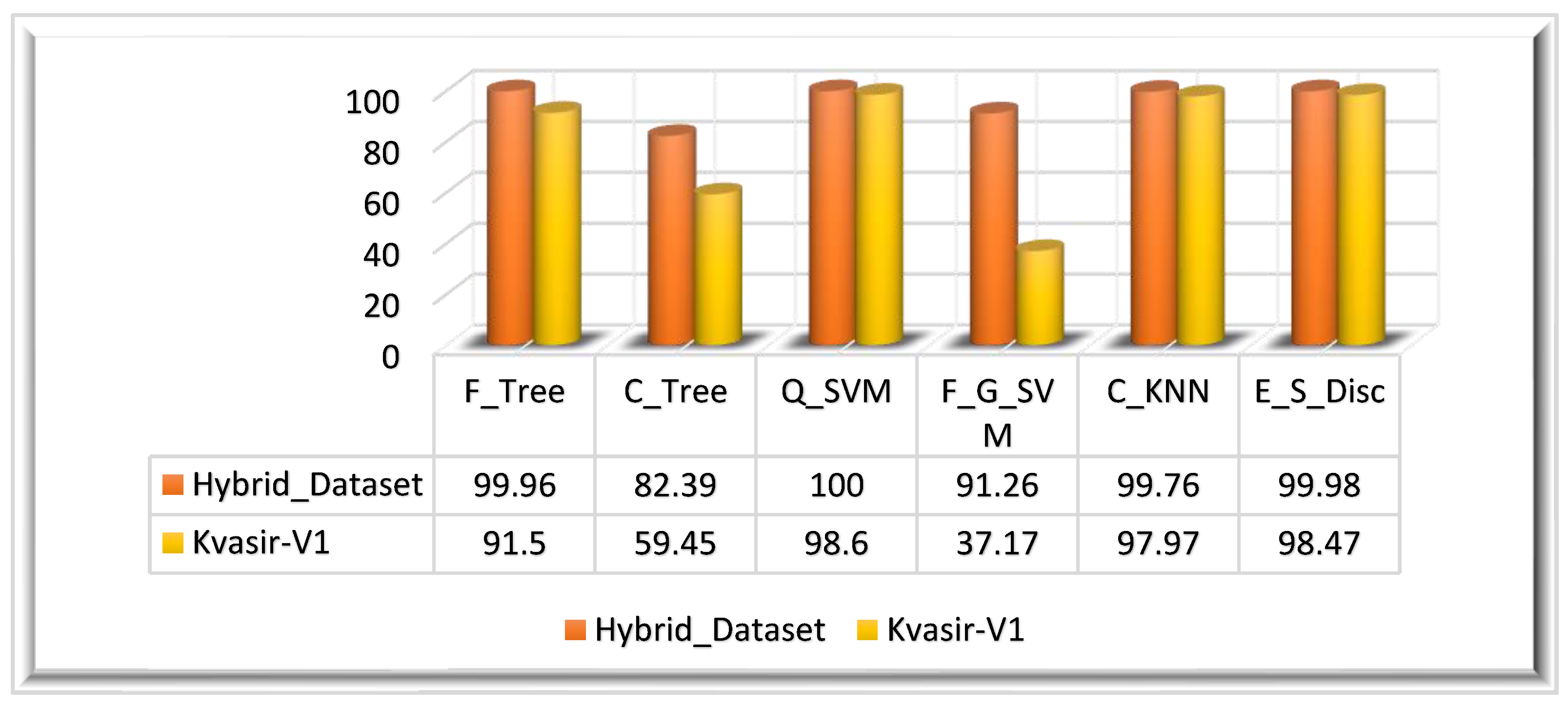
| Hybrid_Dataset | F_Tree | 99.96 | 99.96 | 99.96 | 99.99 | 99.96 | 1.000 | 1.000 | 32.840 |
| C_Tree | 82.39 | 75.45 | 87.64 | 95.66 | 70.22 | 0.75 | 0.790 | 21.435 | |
| Q_SVM | 100.0 | 100.0 | 100.0 | 100.0 | 100.0 | 1.000 | 1.000 | 124.94 | |
| F_G_SVM | 91.26 | 89.04 | 95.34 | 97.54 | 91.25 | 1.000 | 1.000 | 1286.8 | |
| C_KNN | 99.76 | 99.76 | 99.74 | 99.94 | 99.75 | 1.000 | 1.000 | 786.61 | |
| E_S_Disc | 99.98 | 99.98 | 99.98 | 99.99 | 99.98 | 1.000 | 1.000 | 483.66 | |
| Kvasir_V1 | F_Tree | 91.50 | 91.49 | 91.57 | 98.78 | 91.52 | 1.000 | 1.000 | 20.989 |
| C_Tree | 59.45 | 59.45 | 65.68 | 94.2 | 55.35 | 0.7142 | 0.7412 | 17.428 | |
| Q_SVM | 98.60 | 98.60 | 98.60 | 99.80 | 98.60 | 1.000 | 1.000 | 41.758 | |
| F_G_SVM | 37.17 | 37.17 | 76.83 | 91.02 | 37.32 | 0.000 | 0.000 | 232.78 | |
| C_KNN | 97.97 | 97.97 | 98.06 | 99.71 | 97.99 | 1.000 | 1.000 | 56.647 | |
| E_S_Disc | 98.47 | 98.47 | 98.47 | 99.78 | 98.47 | 1.000 | 1.000 | 173.25 |
| Dataset Name | Classifier | ACC (%) | SEN (%) | PRE (%) | SPE (%) | F1 (%) | Kappa Score | MCC | Time (s) |
|---|---|---|---|---|---|---|---|---|---|
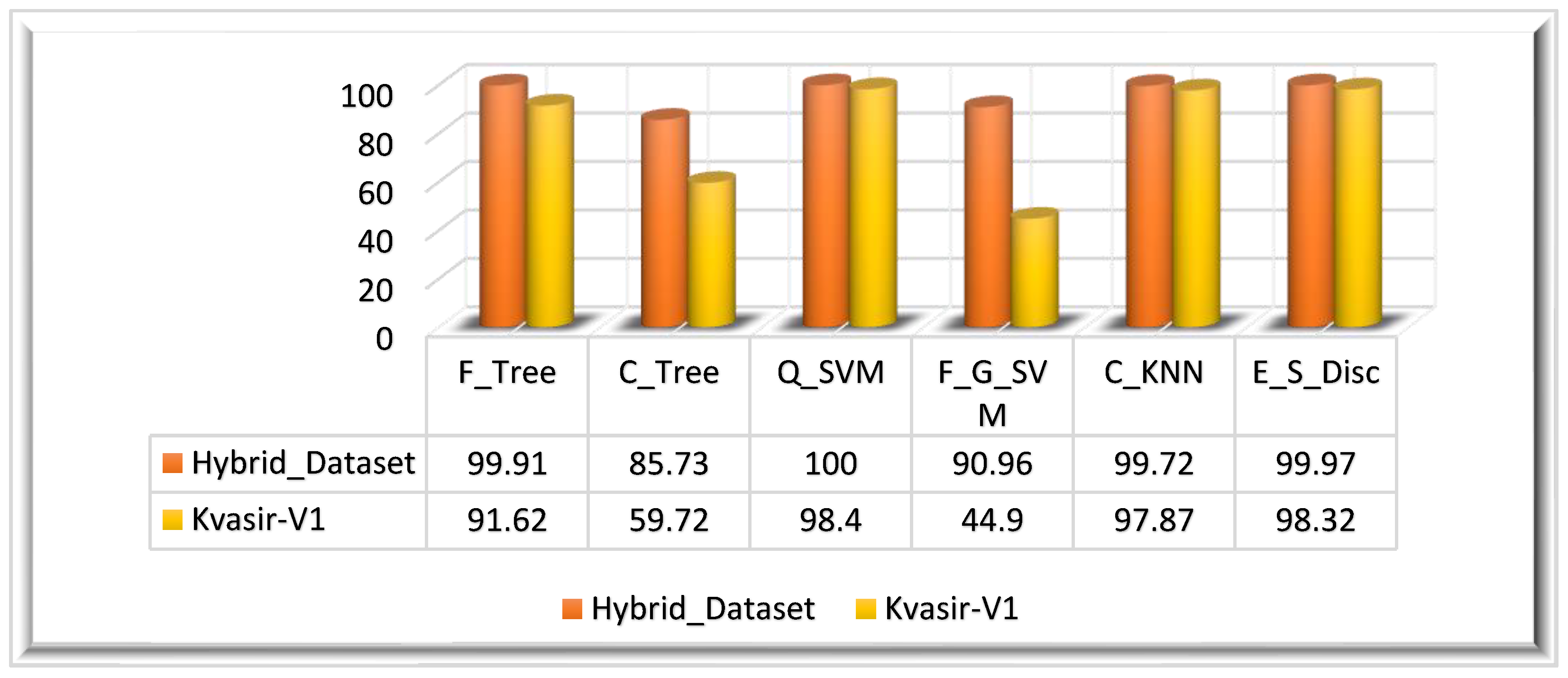
| Hybrid_Dataset | F_Tree | 99.91 | 99.91 | 99.91 | 99.97 | 99.91 | 1.000 | 1.000 | 14.220 |
| C_Tree | 85.73 | 78.75 | 90.95 | 96.45 | 73.94 | 0.750 | 0.791 | 7.8833 | |
| Q_SVM | 100.0 | 100.0 | 100.0 | 100.0 | 100.0 | 1.000 | 1.000 | 58.140 | |
| F_G_SVM | 90.96 | 88.67 | 95.22 | 97.46 | 90.93 | 1.000 | 1.000 | 506.73 | |
| C_KNN | 99.72 | 99.73 | 99.70 | 99.93 | 99.71 | 1.000 | 1.000 | 264.70 | |
| E_S_Disc | 99.97 | 99.97 | 99.97 | 99.99 | 99.97 | 1.000 | 1.000 | 114.66 | |
| Kvasir_V1 | F_Tree | 91.62 | 91.62 | 91.82 | 98.80 | 91.71 | 1.000 | 1.000 | 12.289 |
| C_Tree | 59.72 | 59.72 | 77.70 | 94.24 | 47.16 | 0.571 | 0.604 | 11.308 | |
| Q_SVM | 98.40 | 98.40 | 98.37 | 99.77 | 98.38 | 1.000 | 1.000 | 22.685 | |
| F_G_SVM | 44.90 | 44.90 | 73.70 | 92.12 | 42.78 | 0.428 | 0.495 | 92.103 | |
| C_KNN | 97.87 | 97.89 | 97.97 | 99.69 | 97.92 | 1.000 | 1.000 | 28.063 | |
| E_S_Disc | 98.32 | 98.32 | 98.32 | 99.76 | 98.32 | 1.000 | 1.000 | 66.739 |
| Dataset Name | Classifier | ACC (%) | SEN (%) | PRE (%) | SPE (%) | F1 (%) | Kappa Score | MCC | Time (s) |
|---|---|---|---|---|---|---|---|---|---|
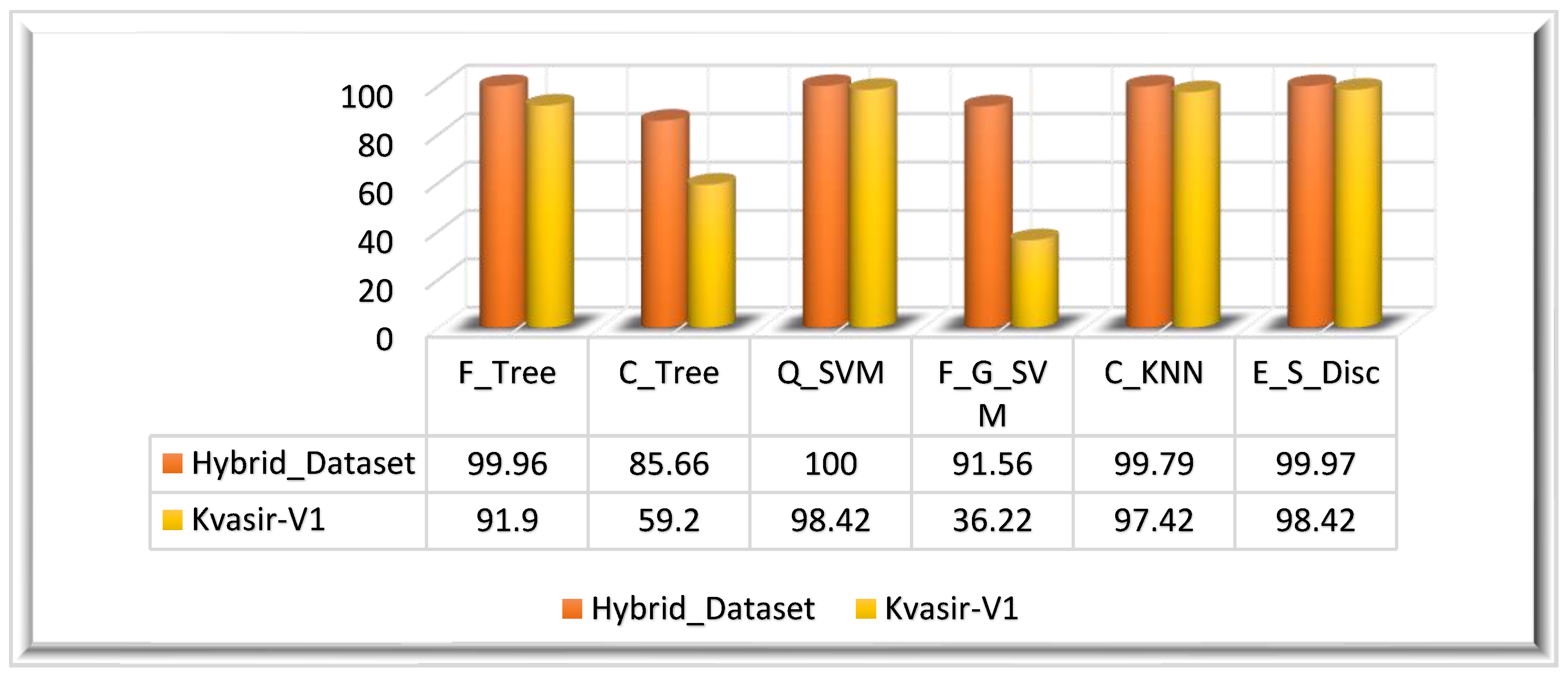
| Hybrid_Dataset | F_Tree | 99.96 | 99.96 | 99.96 | 99.99 | 99.96 | 1.000 | 1.000 | 11.559 |
| C_Tree | 85.66 | 78.68 | 90.82 | 96.44 | 73.85 | 0.750 | 0.791 | 11.000 | |
| Q_SVM | 100.0 | 100.0 | 100.0 | 100.0 | 100.0 | 1.000 | 1.000 | 67.941 | |
| F_G_SVM | 91.56 | 89.31 | 95.46 | 97.63 | 91.45 | 1.000 | 1.000 | 563.31 | |
| C_KNN | 99.79 | 99.8 | 99.76 | 99.94 | 99.78 | 1.000 | 1.000 | 302.73 | |
| E_S_Disc | 99.97 | 99.97 | 99.97 | 99.99 | 99.97 | 1.000 | 1.000 | 135.34 | |
| Kvasir_V1 | F_Tree | 91.90 | 91.90 | 92.02 | 98.84 | 91.95 | 1.000 | 1.000 | 13.461 |
| C_Tree | 59.20 | 59.20 | 74.32 | 94.17 | 50.62 | 0.571 | 0.625 | 5.6968 | |
| Q_SVM | 98.37 | 98.37 | 98.35 | 99.76 | 98.36 | 1.000 | 1.000 | 36.044 | |
| F_G_SVM | 36.22 | 36.22 | 77.41 | 90.88 | 36.23 | 0.000 | 0.000 | 102.24 | |
| C_KNN | 97.42 | 97.45 | 97.58 | 99.63 | 97.47 | 1.000 | 1.000 | 28.223 | |
| E_S_Disc | 98.42 | 98.42 | 98.45 | 99.77 | 98.43 | 1.000 | 1.000 | 60.429 |
| Dataset Name | Classifier | ACC (%) | SEN (%) | PRE (%) | SPE (%) | F1 (%) | Kappa Score | MCC | Time (s) |
|---|---|---|---|---|---|---|---|---|---|
| Hybrid_Dataset | F_Tree | 99.92 | 99.92 | 99.91 | 99.98 | 99.92 | 1.000 | 1.000 | 13.431 |
| C_Tree | 85.81 | 78.87 | 91.13 | 96.47 | 73.98 | 0.750 | 0.791 | 9.9464 | |
| Q_SVM | 100.0 | 100.0 | 100.0 | 100.0 | 100.0 | 1.000 | 1.000 | 64.238 | |
| F_G_SVM | 91.55 | 89.26 | 95.46 | 97.62 | 91.4 | 1.000 | 1.000 | 560.76 | |
| C_KNN | 99.77 | 99.77 | 99.75 | 99.94 | 99.76 | 1.000 | 1.000 | 296.58 | |
| E_S_Disc | 99.93 | 99.93 | 99.93 | 99.98 | 99.93 | 1.000 | 1.000 | 132.16 | |
| Kvasir_V1 | F_Tree | 91.15 | 91.15 | 91.21 | 98.73 | 91.17 | 1.000 | 1.000 | 11.495 |
| C_Tree | 58.82 | 58.82 | 64.93 | 94.11 | 53.31 | 0.704 | 0.7313 | 7.3797 | |
| Q_SVM | 99.24 | 98.69 | 98.69 | 99.87 | 98.69 | 1.000 | 1.000 | 23.957 | |
| F_G_SVM | 39.07 | 39.07 | 78.32 | 91.29 | 39 | 0.142 | 0.285 | 92.005 | |
| C_KNN | 97.62 | 97.62 | 97.71 | 99.66 | 97.65 | 1.000 | 1.000 | 25.571 | |
| E_S_Disc | 98.45 | 98.45 | 98.47 | 99.77 | 98.46 | 1.000 | 1.000 | 66.56 |
| Ref. No. | Year | Dataset | Total Images | Dataset Classes | ACC (%) | SEN (%) | PRE (%) | SPE (%) | F1-Score | Time (s) |
|---|---|---|---|---|---|---|---|---|---|---|
| [3] | 2020 | CUI WAH WCE | 6000 | 3 | 98.40 | 98.33 | 98.36 | - | 98.34 | - |
| [1] | 2021 | CUI WAH WCE | 4500 | 3 | 99.54 | 100.0 | 99.51 | - | - | 31.700 |
| [19] | 2021 | Kvasir-V1 | 4000 | 8 | 87.80 | 87.40 | 87.99 | 98.06 | 87.63 | 50.700 |
| CUI WAH WCE | 2326 | 3 | 99.80 | 99.83 | 99.80 | 99.92 | 99.81 | 17.031 | ||
| [33] | 2021 | CUI WAH WCE | 4000 | 4 | 99.80 | 99.00 | 99.25 | - | 99.12 | 211.90 |
| [35] | 2021 | Kvasir-V1 | 4000 | 8 | 99.25 | 99.30 | 99.89 | 99.25 | - | 24.958 |
| Nerthus | 5524 | 4 | 99.90 | 99.75 | 99.84 | 99.94 | - | 35.033 | ||
| CUI WAH WCE | 2326 | 3 | 100.0 | 100.0 | 100.0 | 100.0 | - | 7.5840 | ||
| [43] | 2021 | Hybrid Dataset | 15,000 | 5 | 99.50 | 99.50 | 96.00 | - | 97.70 | 48.830 |
| [56] | 2021 | Kvasir-V1 | 4000 | 8 | 97.00 | 96.80 | - | 99.20 | - | - |
| [57] | 2022 | Kvasir-V1 | 4000 | 8 | 96.46 | 94.46 | 94.46 | - | 94.46 | - |
| [42] | 2022 | CUI WAH WCE | 4000 | 8 | 99.42 | - | - | - | - | 91.013 |
| Kvasir-V1 | 4000 | 8 | 97.85 | - | - | - | - | 71.031 | ||
| Kvasir-V2 | 8000 | 8 | 97.20 | - | - | - | - | 111.13 | ||
| [58] | 2022 | Kvasir-V1 | 4000 | 8 | 98.20 | - | - | - | - | 52.504 |
| Kvasir-V2 | 8000 | 8 | 98.02 | - | - | - | - | 102.502 | ||
| CUI WAH WCE | - | 3 | 99.61 | - | - | - | - | 69.544 | ||
| Proposed | Hybrid Dataset | 15,448 | 5 | 100.0 | 100.0 | 100.0 | 100.0 | 100.0 | 58.140 | |
| Kvasir-V1 | 4000 | 8 | 99.24 | 98.69 | 98.69 | 99.87 | 98.69 | 23.957 | ||
Disclaimer/Publisher’s Note: The statements, opinions and data contained in all publications are solely those of the individual author(s) and contributor(s) and not of MDPI and/or the editor(s). MDPI and/or the editor(s) disclaim responsibility for any injury to people or property resulting from any ideas, methods, instructions or products referred to in the content. |
© 2023 by the authors. Licensee MDPI, Basel, Switzerland. This article is an open access article distributed under the terms and conditions of the Creative Commons Attribution (CC BY) license (https://creativecommons.org/licenses/by/4.0/).
Share and Cite
Naz, J.; Sharif, M.I.; Sharif, M.I.; Kadry, S.; Rauf, H.T.; Ragab, A.E. A Comparative Analysis of Optimization Algorithms for Gastrointestinal Abnormalities Recognition and Classification Based on Ensemble XcepNet23 and ResNet18 Features. Biomedicines 2023, 11, 1723. https://doi.org/10.3390/biomedicines11061723
Naz J, Sharif MI, Sharif MI, Kadry S, Rauf HT, Ragab AE. A Comparative Analysis of Optimization Algorithms for Gastrointestinal Abnormalities Recognition and Classification Based on Ensemble XcepNet23 and ResNet18 Features. Biomedicines. 2023; 11(6):1723. https://doi.org/10.3390/biomedicines11061723
Chicago/Turabian StyleNaz, Javeria, Muhammad Imran Sharif, Muhammad Irfan Sharif, Seifedine Kadry, Hafiz Tayyab Rauf, and Adham E. Ragab. 2023. "A Comparative Analysis of Optimization Algorithms for Gastrointestinal Abnormalities Recognition and Classification Based on Ensemble XcepNet23 and ResNet18 Features" Biomedicines 11, no. 6: 1723. https://doi.org/10.3390/biomedicines11061723
APA StyleNaz, J., Sharif, M. I., Sharif, M. I., Kadry, S., Rauf, H. T., & Ragab, A. E. (2023). A Comparative Analysis of Optimization Algorithms for Gastrointestinal Abnormalities Recognition and Classification Based on Ensemble XcepNet23 and ResNet18 Features. Biomedicines, 11(6), 1723. https://doi.org/10.3390/biomedicines11061723