Article

Detection of Mackerel Fish Spoilage with a Gas Sensor Based on One Single SnO2 Nanowire

by
Matteo Tonezzer
1,2,3,4
1
Department of Food Quality and Nutrition, Research and Innovation Centre, Fondazione Edmund Mach, via E. Mach 1, 38010 San Michele all’Adige, Italy
2
Dipartimento di Ingegneria Civile Ambientale e Meccanica, University of Trento, Via Mesiano 77, 38123 Trento, Italy
3
Center Agriculture Food Environment, University of Trento/Fondazione Edmund Mach, via E. Mach 1, 38010 San Michele all’Adige, Italy
4
IMEM-CNR, Sede di Trento-FBK, Via alla Cascata 56/C, 38123 Povo-Trento, Italy
Chemosensors 2021, 9(1), 2; https://doi.org/10.3390/chemosensors9010002
Submission received: 1 December 2020 / Revised: 17 December 2020 / Accepted: 21 December 2020 / Published: 23 December 2020
(This article belongs to the Special Issue Nanomaterials-Based Sensors)

Abstract

:
A chemosensor consisting of one single tin oxide nanowire is used to determine the freshness status of mackerel fish (Scomber scombrus) in a quick and non-invasive way. The tiny chemoresistive sensor is first tested with pure ammonia and then used to measure the total volatile basic nitrogen from different samples of fish at different degrees of freshness. The sensor has proved capable of determining the freshness of a sample in few seconds compared to traditional methods such as microbial count and chromatography, which take hours. The sensor response is well correlated with the total viable count (TVC), proving that the total volatile basic nitrogen is a good way to quickly test the bacterial population in the sample. After calibrating the sensor (following the degradation of the fish during almost two days), it has been tested with random double blind samples, proving that it can well discriminate the degree of freshness of the fish preserved at different temperatures.

1. Introduction

Food has a profound impact on people’s health, chronic disease risk, and longevity. Better nutritional quality is achieved also by consuming more fresh products instead of highly processed foods with additives (artificial food colors, preservatives, etc.). Unfortunately, fresh food is subject to deterioration quite rapidly, and this has important repercussions not only on the food industry, but also on the health of consumers, with social and health costs [1,2]. Recently, the globalization and the centralization of many production chains has led to greater distances between the production areas and the consumer and more complex supply chains [3]. Fish is a food that, also thanks to its healthy properties, is consumed more and more all over the world [4]. For these reasons, it is increasingly important to develop cheaper and faster non-invasive methods to assess fish freshness during real time. Until a few years ago, panels of human experts evaluating appearance, smell, and texture were used [5,6], but this type of procedure is laborious and not always reliable, which is why the use of sensors has recently become essential.
The main factor limiting the shelf life of fresh fish is the activity of microorganisms. For this reason, an estimate of total vital counts (TVC) is generally used as a reference and as a definitive index [7]. After the death of the fish, the amount of microorganisms on its surface increases and gradually spreads to various tissues [8]. Several methods have been used to measure the freshness of the fish [5,9]. As microorganisms degrade fish tissues, they convert trimethylamine oxide into (CH3)3N (trimethylamine or TMA) and (CH3)2NH (dimethylamine or DMA). At the same time, NH3 (ammonia) is produced through the decomposition of urea and amino acids by bacteria [10]. These volatiles are collectively referred to as TVB-N (total volatile basic nitrogen), and their concentration is considered a good indicator of fish freshness. Among the most used and accurate systems to analyze volatile compounds are the headspace methods, which consist of extracting the volatiles and then separating them and identifying them with chromatographic techniques [5].
Unfortunately, these methods are time-consuming and require trained personnel and equipment accessible only in the laboratory. So, this type of analysis can only be done on a sample basis, guaranteeing the freshness of only a small part of the products. Therefore, it is important to develop non-invasive sensors that are small, cheap, and fast, in order to be able to extensively monitor the supply chain in real time. A suitable tool for this task, as it is able to distinguish complex gas mixtures, is the electronic nose: an array of sensors whose responses are combined together [11,12]. These devices are able to distinguish complex mixtures of volatile organic compounds that make up the aroma of an agro-food product. Electronic noses are able to distinguish complex mixtures of volatiles and therefore many different agro-food products [13,14,15]. In this case, it is not necessary to evaluate subtle nuances but to measure a very precise marker (the TVB-N), and therefore a single sensor can be smaller, cheaper, and easily integrated. Chemoresistors based on semiconducting metal oxides (SMOs) are ideal candidates for this task: their dimensions are less than one micron, and they are very simple, since they are basically a resistance that varies by reacting to the atmosphere around them. Therefore, they can be easily integrated into portable or wearable devices (mobile phones or smart watches) or into containers used for transporting fish. The mechanism underlying their detection performance was presented by Seyama [16], and the latest generation consists of SMO nanostructures. The enormous surface/volume ratio of the nanostructures (usually nanowires, NWs) greatly improves the detection performance, allowing gases to be detected down to ranges below ppm (parts per million). Nanowires can be used as a porous thin film [17] that is grown directly from the electrodes [18] or even contacted individually [19].
In the present work, the latter method will be used in order to exploit the sensitivity and the speed of response and recovery of a single nanowire. Using the microbial count as a reference, the nanosensor has been shown to be able to measure mackerel freshness non-invasively, quickly, and accurately.

2. Materials and Methods

2.1. Synthesis of SnO2 Nanowires

The tin oxide (SnO2) nanowires were grown in a horizontal quartz tube placed inside a furnace (Lindberg Blue M, Thermo Fisher Scientific, Waltham, MA, USA) by chemical vapor deposition (CVD). An alumina boat filled with pure tin monoxide was used as an evaporation source and placed in the center of the furnace at its maximum temperature. A silicon wafer square (about 1 × 1 cm2) was used as substrate, deposited with a thin gold film (about 5 nm) acting as a catalyst, and positioned 1 cm from the alumina boat. The quartz tube was cleaned by pumping it down to 10−2 mbar and purging it with high-purity (99.999%) argon. This cycle was repeated three times, and finally, the system was pumped down to its limit pressure. Then, the temperature was increased from room temperature (26 °C) to 850 °C with a slope of 25 °C per minute, and the furnace was left for five minutes at 850 °C to thermalize. Then, an oxygen flow of 0.35 standard cubic centimeters (sccm) was flowed into the system, starting the process. Growth of the NWs lasted 30 min; then, the system was shut down and allowed to cool. Once the growth was complete, the samples showed a soft and homogeneous white film.

2.2. Material Characterization

The thin white film grown via CVD was characterized by X-ray diffraction (XRD) using a Philips Xpert Pro (PANalytical, Westborough, MA, USA) working at 40 kV with CuKα radiation. Transmission electron microscopy (TEM) investigation was carried out using a JEM-100CX (JEOL, Tokyo, Japan) operating at 90 kV, and secondary electron microscopy (SEM) images were acquired with a Hitachi S-4800 (Hitachi, Krefeld, Germany).

2.3. Fabrication of the Sensor

Then, a piece of the white thin film (a forest of spaghetti-like nanowires) was sonicated in dimethylformamide for two seconds. The resulting dispersion was dropped onto a Si/SiO2 wafer by spinning it at 6000 rpm in order to obtain the desired NW density. A matrix of Ti/Pt (10/250 nm) electrodes was patterned on the dispersed nanowires using the standard UV lithography technique on the whole wafer.
The pairs of electrodes connected by nanowires were found by combining two tests: resistance measurement and optical microscopy. The best candidates for single nanowire devices were characterized by SEM imaging to verify their morphology, and the best was chosen to be used as a gas sensor.

2.4. Gas Sensor Measurements

The single-nanowire sensor was measured in a home-built system comprising a measuring chamber with heatable sensor holder and micro-probes, gas flow controllers connected to high-purity gas bottles, and a multimeter (Keithely 2410, Keithely, Cleveland, Ohio, USA) connected to a data acquisition program (LabView, National Instruments). The device was first thermally conditioned for 4 h at 500 °C in nitrogen while powered at 1V to stabilize the nanostructures and their base resistance. This is to ensure that the electrical properties of the nanostructures do not change during subsequent measurements [20]. Then, the electrical contact of the SnO2 nanowire with the titanium/platinum electrodes was studied by analyzing the I-V curves. Good linear behavior was found, which demonstrated good ohmic contact. The sensor resistance drops from 4.25 to 1.43 to 0.66 MΩ when measured at 200, 250, and 300 °C.
The sensor was operated under a voltage of 1V, while different temperature values (200, 250, and 300 °C) were set by the heater on the sample holder. Different concentrations of ammonia (10, 5, 2, 1, and 0.5 parts per million, ppm) were tested while maintaining the total gas flow of 400 sccm. The sensor response was defined as S = Rair/Rgas, where Rgas and Rair are the resistance of the sensor with ammonia or in air, respectively. The speed of the single nanowire sensor is measured using the definition of response and recovery times: the time necessary to reach 90% of the maximum response and to get down to 90% of the complete recovery, respectively. The limit of detection (LoD) was calculated as 3·noiserms/slope, where noiserms is the standard deviation of the sensor signal and slope is the derivative of the sensor response as a function of ammonia concentration.

2.5. Mackerel Spoilage Measurements

Several small cubes of mackerel fish weighting 20 g were cut from a fresh fillet using disposable gloves and autoclaved tools. Each cube is kept in a different glass jar until the measurement with the gas sensor (some at room temperature = 25 °C and some in a fridge at 4 °C). Every two hours, a fish sample was inserted into the sensing chamber to determine its TVB-N, and immediately afterwards, it was subjected to microbial analysis in order to compare the two measurements. The total viable count (TVC) was evaluated using a spread plate method [21] on a plate count agar and agar base (Oxoid CM0463 and 0055, Thermo Fisher Scientific, Waltham, MA, USA). Then, the plates were counted after an incubation time of 48 h at 30 °C.

3. Results and Discussion

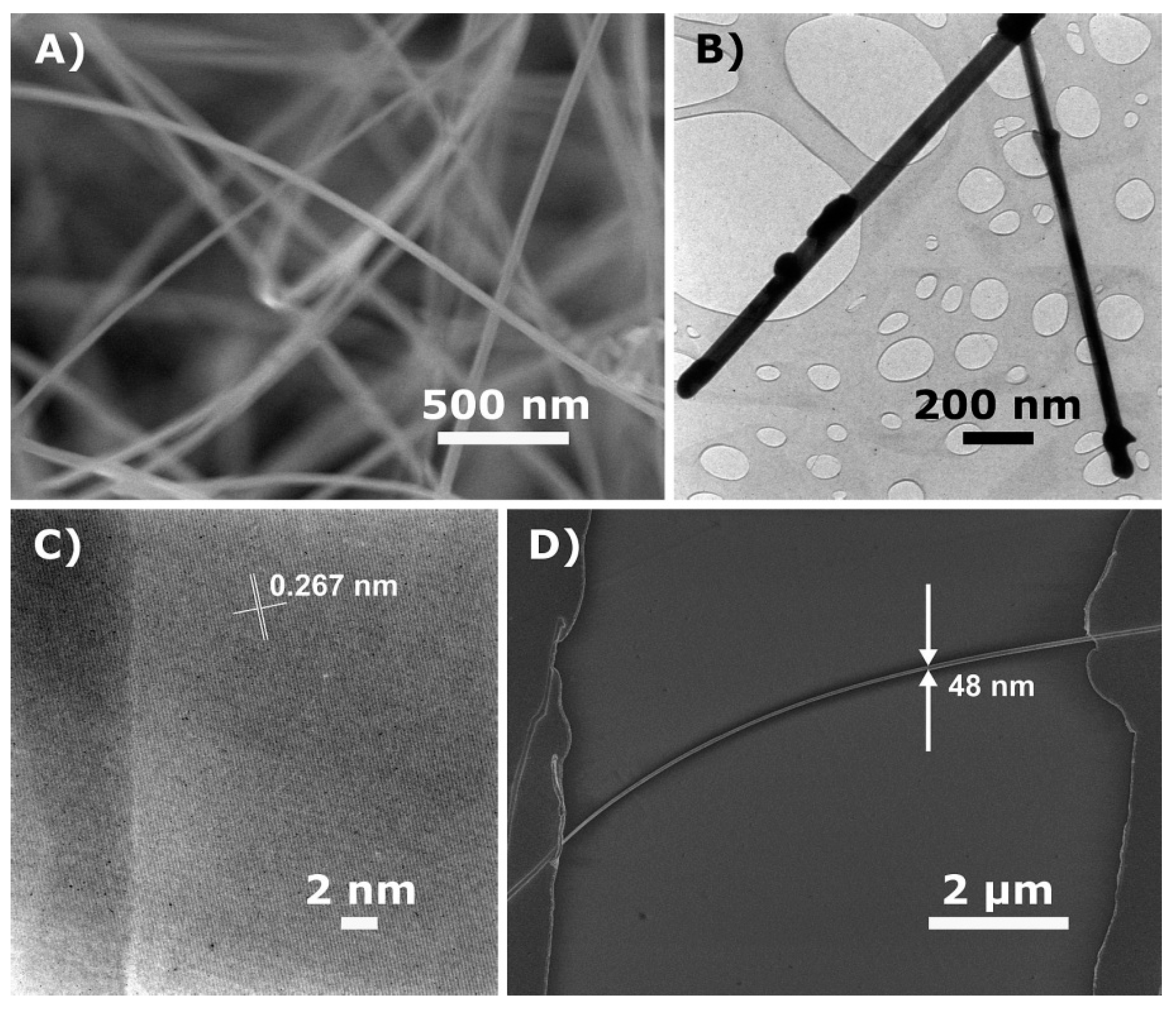
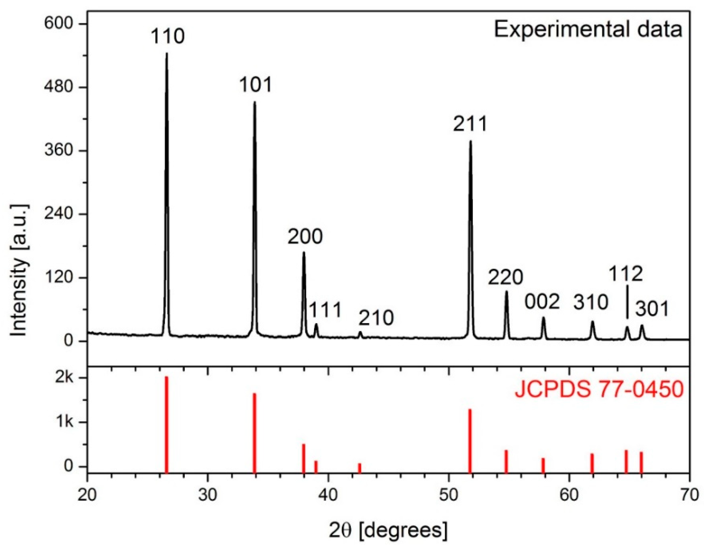
3.1. Nanowires Characterization

The SnO2 nanowires composing the white soft layer obtained by CVD were first investigated by scanning electron microscopy to characterize their morphology. A SEM image of the spaghetti-like nanowires is shown in Figure 1A.
As can be seen, the nanowires are long, smooth, and straight, with an average diameter of 50 nm. Figure 1B shows a TEM image of two nanowires, confirming their smooth and straight shape, their single-crystallinity, and their constant diameter. The HR-TEM of a nanowire in Figure 1C shows inter-planar fringes of 0.269 nm, corresponding to the (101) crystal planes of tetragonal SnO2 structure. Figure 1D illustrates a single nanowire bridging two metal electrodes. The gap between the Ti/Pt pads is 8 μm wide, while the diameter of the nanowire is approximately 48 nm.
The composition and structure of the nanowires were also determined by X-ray diffraction, as shown in Figure 2.
All the diffraction peaks in the pattern can be readily indexed to the tetragonal phase of SnO2 with lattice parameters of a = b = 4.742 Å and c = 3.186 Å, which agree well with the reported values (JCPDS no. 77-0450). No amorphous contributions or impurity peaks can be observed nor other phases of SnO2, confirming the high purity of the nanowires.

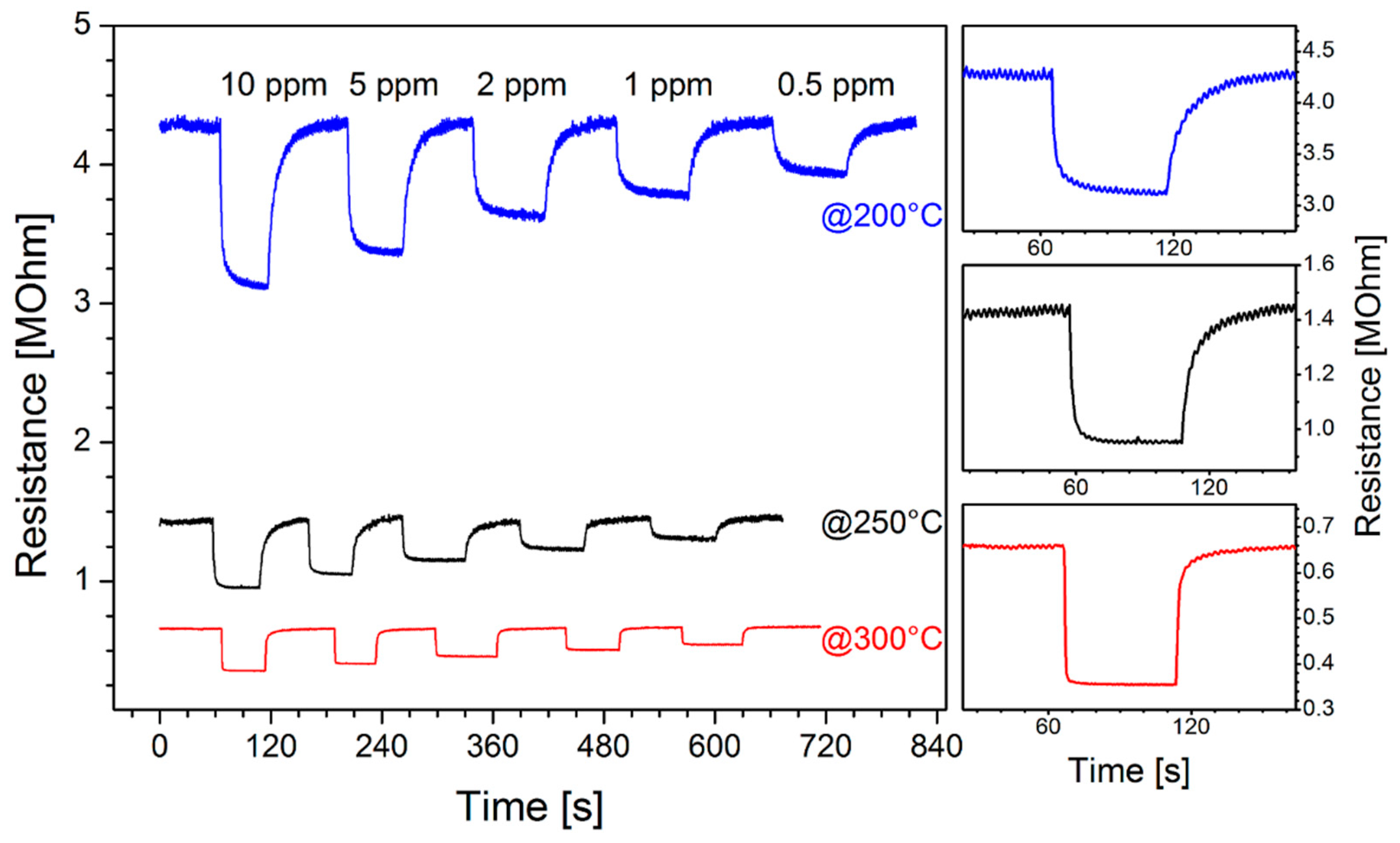
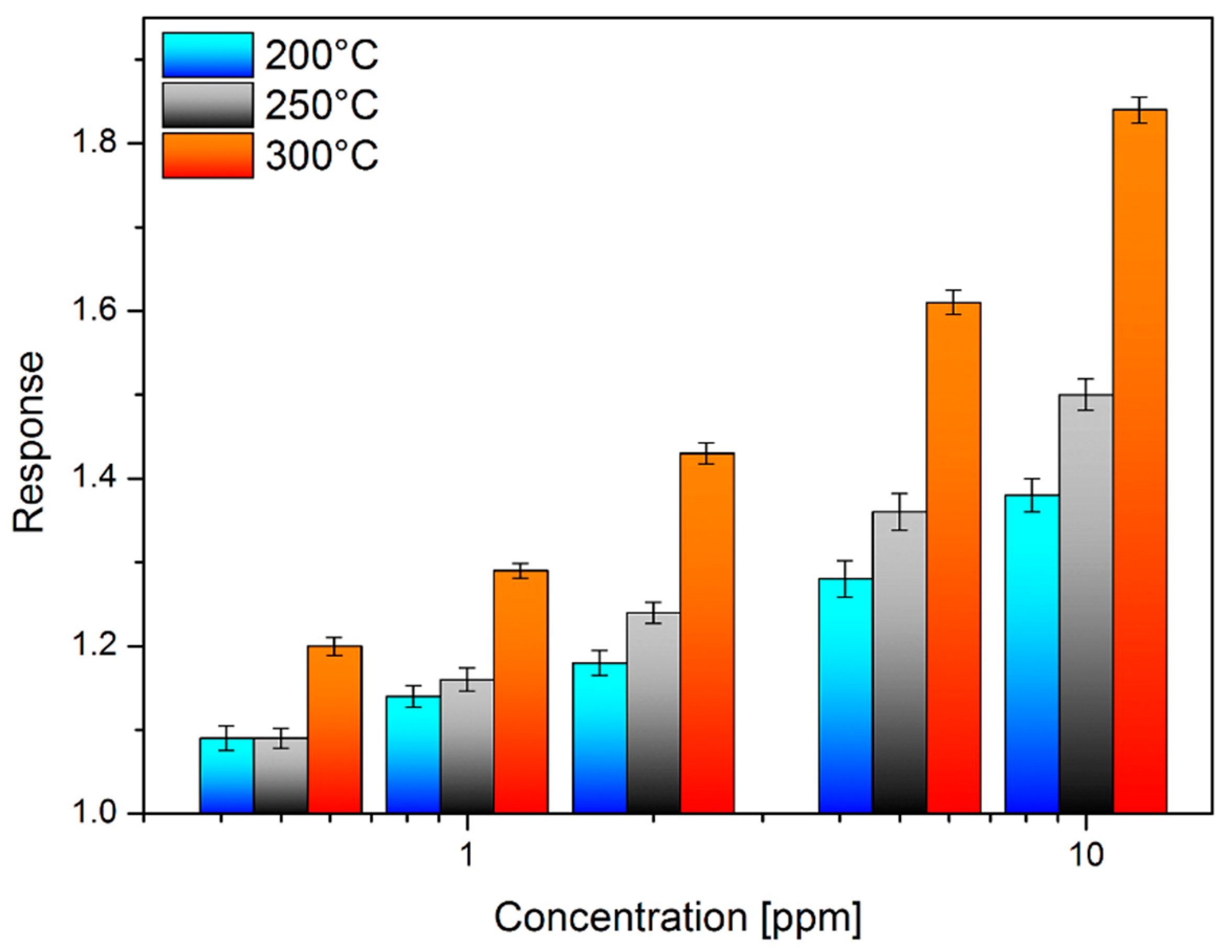
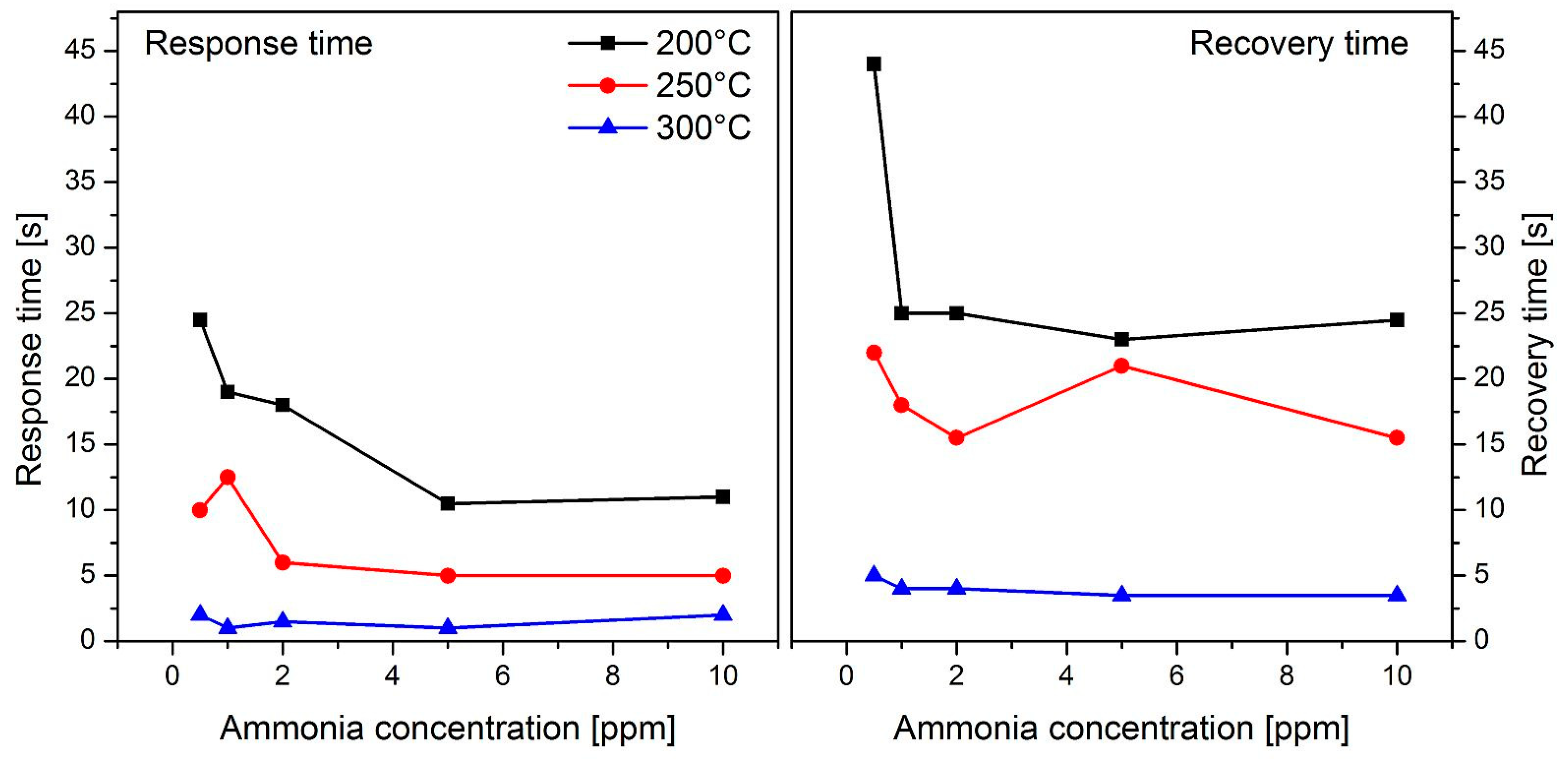
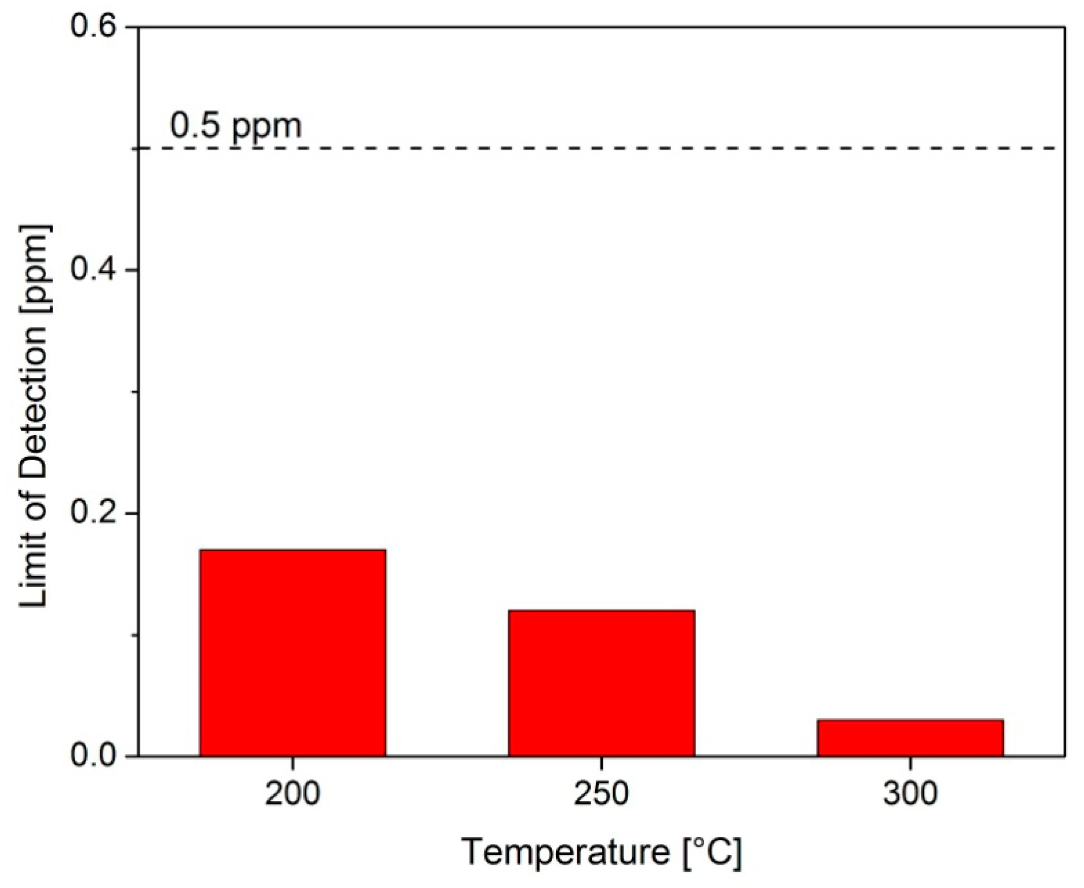
3.2. Ammonia Sensing Performance

In order to check the sensor performance at different working temperatures, the resistance of the single SnO2 nanowire was dynamically measured at three temperature values: 200, 250, and 300 °C. The plots are shown in Figure 3.
The resistance of the nanowire decreases with increasing temperature (from 4.3 MOhm at 200 °C to 0.7 MOhm at 300 °C). Therefore, the power consumed by the sensor is always of the order of μW: 0.23 μW at 200 °C and 1.43 μW at 300 °C.
At any working temperature, the resistance of the nanosensor is constant in the air and decreases sharply when ammonia gas is injected into the system. The resistance returns to its previous value when the ammonia flow is stopped and air is returned to the system. This behavior can be easily explained, as SnO2 is an n-type semiconductor, and it is very reactive to its surroundings [22], mainly to reducing gases such as ammonia [23]. The sensing mechanism is well known: as soon as the nanowire is exposed to air, oxygen is adsorbed on its surface in the form of O and O2−, draining electrons from the NW and increasing its resistance. When ammonia molecules are flowed onto the nanowire surface, they react with the adsorbed oxygen atoms, releasing electrons back to the nanostructure and decreasing the nanostructure resistance:
2NH3 + 3O(ads) → N2 + 3H2O + 3e
It can easily be seen that the intensity of the response decreases with decreasing gas concentration (ammonia is injected at 10, 5, 2, 1, and 0.5 ppm, in order).
The responses were calculated by averaging the values obtained from three measurement runs such as that shown in Figure 3, which were carried out on three different days. The values obtained are shown in Figure 4, where the root mean square error (RMSE) is indicated for each concentration at each temperature.
The response values calculated from the three graphs are shown in Figure 4 in order to be compared. The response is higher when the sensor works at a higher temperature.
Another thing that can be seen in Figure 3 is how both the response and the recovery of the sensor start very abruptly, but then, the behavior changes according to the temperature at which the device is working. These parameters have also been calculated (as explained in Section 2.4.) so that they can be quantitatively compared, and they are shown in Figure 5.
As can be seen, response times are always lower than 25 s, while recovery times are lower than 45 s and in general longer than response times in the same conditions. Both parameters seem to decrease somewhat as the gas concentration increases but without a marked trend. It is clear that the sensor speed increases as the operating temperature increases, and the best conditions are achieved at 300 °C, with response times around 2 s and response times around 4 s. The limit of detection was calculated applying the definition given in Section 2.4, and the obtained results are shown in Figure 6.
The LoD of the single nanowire device is always less than 1 ppm and decreases with increasing temperature: 170, 120, and 30 ppb at 200, 250, and 300 °C, respectively. This results from a higher response (Figure 4) and a higher signal-to-noise ratio (Figure 3).
In light of the performance obtained by the nanosensor by measuring ammonia, a working temperature of 300 °C was chosen for the subsequent measurements. At this temperature, all sensor parameters are optimized: higher response, faster response and recovery, and lower limit of detection.

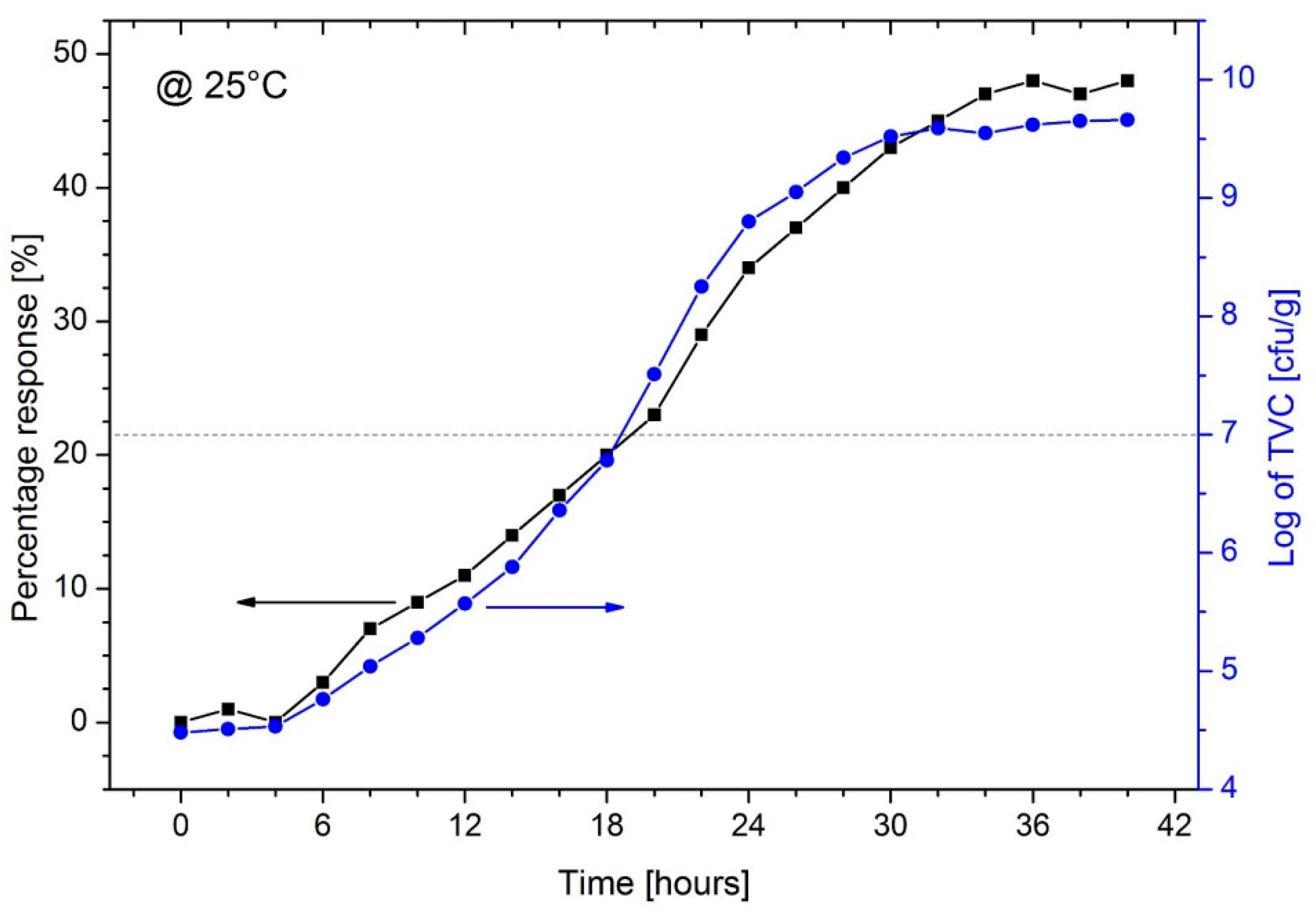
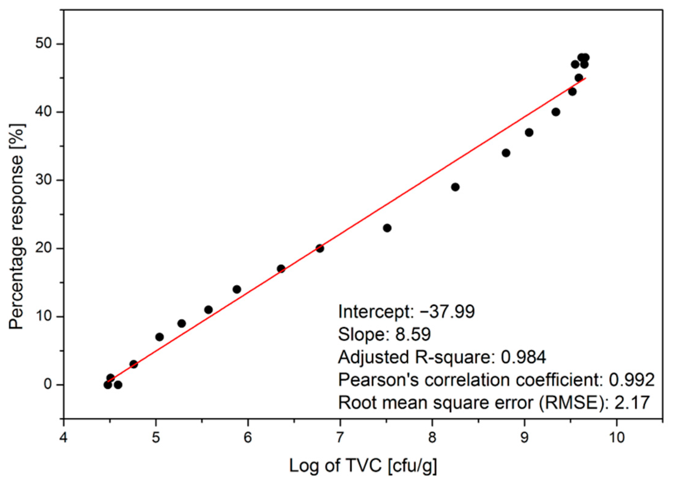
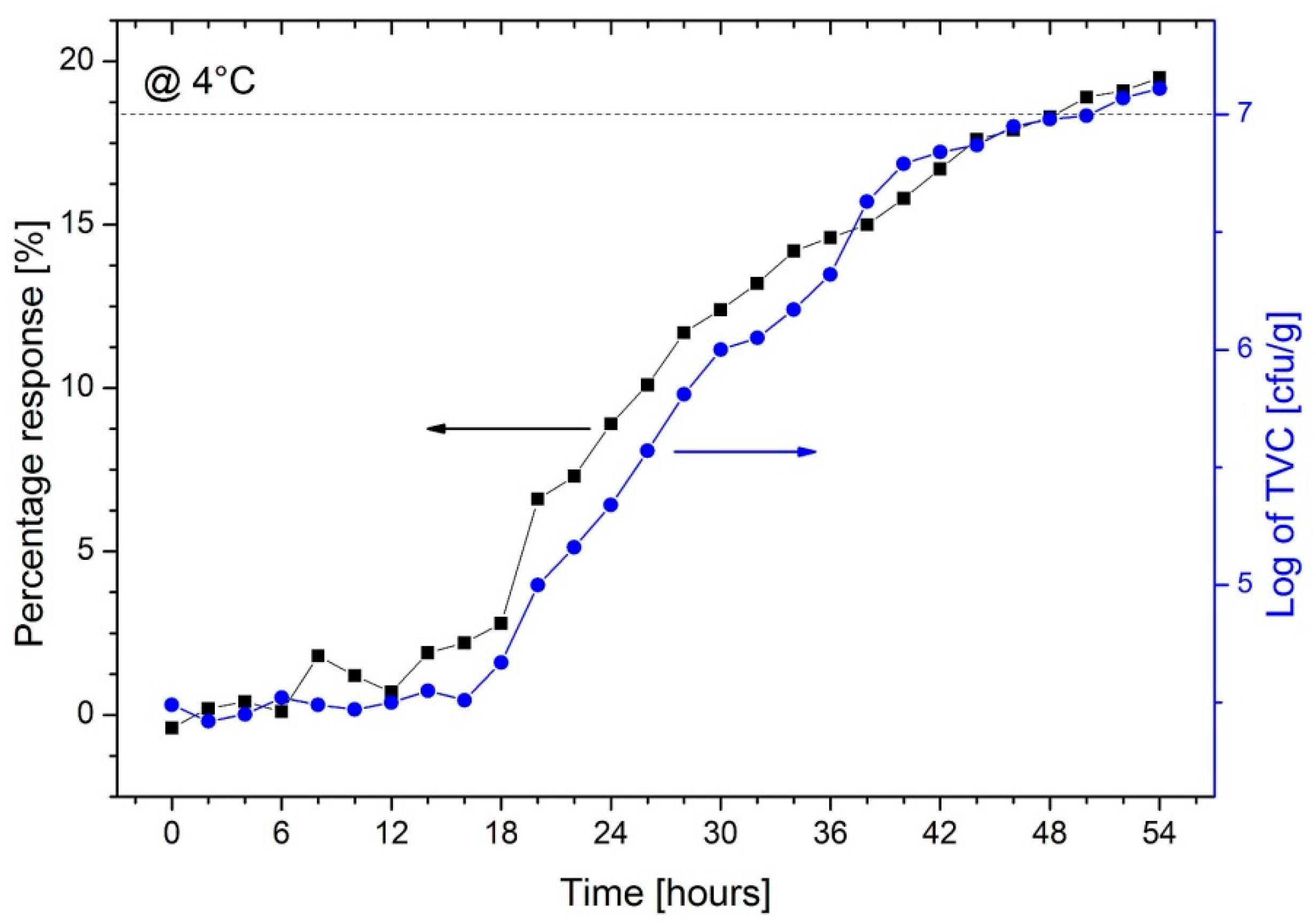
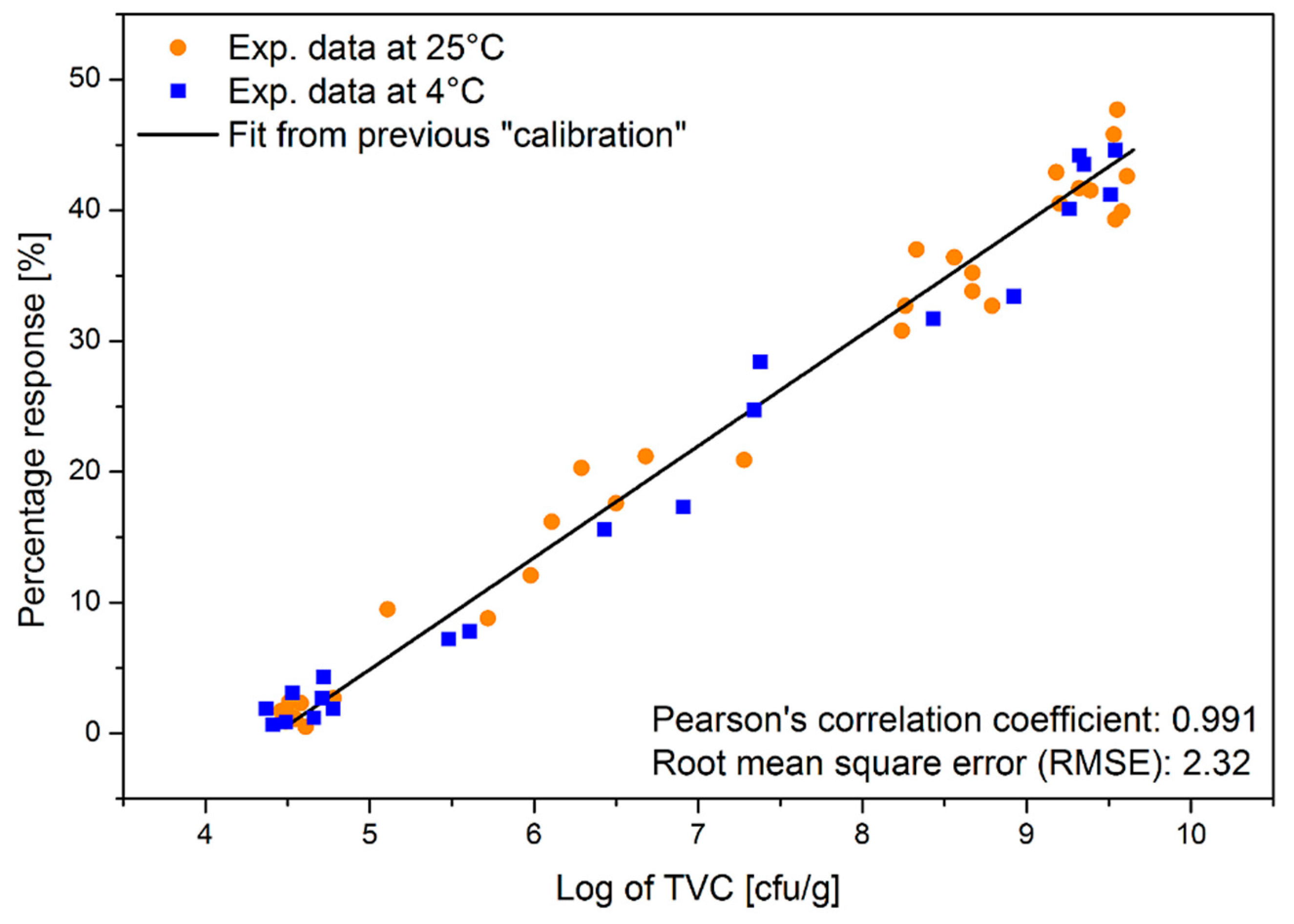
3.3. Mackerel Fish Spoilage Measurements

The response of the gas sensor and the total viable count are plotted together in Figure 7. At the beginning, the TVC starts around 3 × 10⁴ cfu/g and grows slowly; then, it reaches its maximum slope around 18 h, and finally, around 30 h, it seems to stabilize around 3 × 10⁹ cfu/g.
The nanosensor response follows a similar behavior, increasing with a smaller slope and with a less sharp stabilization at the end. It is clear that the sensor response can be considered a good approximation of the total viable count. The horizontal dotted line identifies the threshold considered as the end of the shelf life of the fish both in the literature [5,24] and for institutions [25]. In our case, this limit was reached after 18 h of storage at room temperature. The correlation between the gas sensor response and the total viable count is shown in Figure 8.
As can be seen, the two signals are well correlated (correlation coefficient = 0.992) with a small error (RMSE = 2.17%). The root mean square error increases at log(TVC) values higher than 7.5, while below this value, it is much smaller. In particular, it is minimum for log(TVC) values from 6.4 to 7. Since the standard threshold used to distinguish the end of shelf life in literature is log(TVC) = 7, the sensor is more accurate than the total RMSE indicates, and the gas sensor can be calibrated using the total viable count as a reference.
To check how the shelf life of the fish is prolonged by storing it in a domestic refrigerator, spoilage measurements were repeated on samples stored at 4 °C, and the results are shown in Figure 9.
Comparing the plots in Figure 9 with those in Figure 7, it is clear that the deterioration of the mackerel is going much more slowly. Both the gas response and TVC increase very slowly for up to 18 h; then, the slope increases for both signals. The correlation between the two signals is good also in this case (correlation = 0.991), so that also, in this case, the gas response can be considered a good approximation of the total viable count. It appears evident that in this case, the threshold of 107 cfu/g is reached much later, around 48 h of storage.
To check if the sensor calibration works, mackerel samples stored at both 25 and 4 °C were measured at a random spoilage level. The results obtained are shown in Figure 10.
Figure 10 shows that there is a good correlation between the response obtained from the single-nanowire sensor and the bacterial population obtained from the TVC. The Pearson’s correlation coefficient is 0.991, while the root mean square error on the sensor response is 2.32%. Samples stored at room temperature or in the fridge do not appear to have different trends. This confirms that the response of the resistive nanosensor is a good measure of the level of deterioration of the mackerel.

4. Conclusions

A single SnO2 nanowire was used as resistive gas sensor to assess the spoilage of mackerel fish. Performance was initially tested by measuring ammonia concentrations from 0.5 to 10 ppm at three different operating temperatures. At the optimal temperature (300 °C), the sensor responds and recovers quickly (2 and 4 s, respectively) with a limit of detection of 30 ppb. Then, the nanosensor was used to monitor mackerel deterioration over time. The response of the sensor follows well the concentration of the microorganisms while the fish deteriorates, with a correlation of 0.992. The sensor was tested with double-blind measurements of samples stored at 25 °C and 4 °C, and it was able to assess the mackerel quality in all cases.

Funding

This research received no external funding.

Data Availability Statement

The data presented in this study are openly available in Open Science Framework at doi:10.17605/OSF.IO/83SMW.

Acknowledgments

The author acknowledges F. Rossi for the help with the microbial analysis in the Bio-STE Laboratory.

Conflicts of Interest

The authors declare no conflict of interest.

References

  1. Scharff, R.L. Economic burden from health losses due to foodborne illness in the United States. J. Food Prot. 2012, 75, 123–131. [Google Scholar] [CrossRef] [PubMed]
  2. Sundström, K. Cost of Illness for Five Major Foodborne Illnesses and Sequelae in Sweden. Appl. Health Econ. Health Policy 2018, 16, 243–257. [Google Scholar] [CrossRef] [PubMed] [Green Version]
  3. Boyer, D.; Ramaswami, A. Comparing urban food system characteristics and actions in US and Indian cities from a multi-environmental impact perspective: Toward a streamlined approach. J. Ind. Ecol. 2020, 24, 841–854. [Google Scholar] [CrossRef]
  4. The State of World Fisheries and Aquaculture 2020. Sustainability in Action; FAO: Rome, Italy, 2020; ISBN 978-92-5-132692-3. [CrossRef]
  5. Olafsdóttir, G.; Martinsdóttir, E.; Oehlenschläger, J.; Dalgaard, P.; Jensen, B.; Undeland, I.; Mackie, I.M.; Henehan, G.; Nielsen, J.; Nilseng, H. Methods to evaluate fish freshness in research and industry. Trends Food Sci. Technol. 1997, 8, 258–265. [Google Scholar] [CrossRef]
  6. Wojnowski, W.; Majchrzak, T.; Dymerski, T.; Gębicki, J.; Namieśnik, J. Electronic noses: Powerful tools in meat quality assessment. Meat Sci. 2017, 131, 119–131. [Google Scholar] [CrossRef]
  7. Deisingh, A.K.; Stone, D.C.; Thompson, M. Applications of electronic noses and tongues in food analysis. Int. J. Food Sci. Technol. 2004, 39, 587–604. [Google Scholar] [CrossRef]
  8. Wojnowski, W.; Majchrzak, T.; Dymerski, T.; Gębicki, J.; Namieśnik, J. Portable Electronic Nose Based on Electrochemical Sensors for Food Quality Assessment. Sensors 2017, 17, 2715. [Google Scholar] [CrossRef] [Green Version]
  9. Loutfi, A.; Coradeschi, S.; Mani, G.K.; Shankar, P.; Rayappan, J.B.B. Electronic noses for food quality: A review. J. Food Eng. 2015, 144, 103–111. [Google Scholar] [CrossRef]
  10. Macías, M.M.; Agudo, J.; Manso, A.G.; Orellana, C.J.G.; Velasco, H.M.G.; Caballero, R.G. A compact and low cost electronic nose for aroma detection. Sensors 2013, 13, 5528–5541. [Google Scholar] [CrossRef] [Green Version]
  11. Silva, F.; Duarte, A.M.; Mender, S.; Pinto, F.R.; Barroso, S.; Ganhão, R.; Gil, M.M. CATA vs. FCP for a rapid descriptive analysis in sensory characterization of fish. J. Sens. Stud. 2020, e12605. [Google Scholar] [CrossRef]
  12. Jia, S.; Li, Y.; Zhuang, S.; Sun, X.; Zhang, L.; Shi, J.; Hong, H.; Luo, Y. Biochemical changes induced by dominant bacteria in chill-stored silver carp (Hypophthalmichthys molitrix) and GC-IMS identification of volatile organic compounds. Food Microbiol. 2019, 84, 103248. [Google Scholar] [CrossRef] [PubMed]
  13. Gram, L.; Huss, H.H. Microbiological spoilage of fish and fish products. Int. J. Food Microbiol. 1996, 33, 121–137. [Google Scholar] [CrossRef]
  14. Mustafa, F.; Andreescu, S. Chemical and Biological Sensors for Food-Quality Monitoring and Smart Packaging. Foods 2018, 7, 168. [Google Scholar] [CrossRef] [PubMed] [Green Version]
  15. Dikeman, M.; Devine, C. Encyclopedia of Meat Sciences, 2nd ed.; Academic Press: Amsterdam, The Netherlands, 2004; ISBN 978-0124649705. [Google Scholar]
  16. Seyama, T.; Kato, A.; Fujishi, K.; Nagatani, M. A New Detector for Gasous Components Using Semiconductive Thin Films. Anal. Chem. 1962, 34, 1502. [Google Scholar] [CrossRef]
  17. Tonezzer, M.; Le, D.T.T.; Iannotta, S.; Hieu, N.V. Selective discrimination of hazardous gases using one single metal oxide resistive sensor. Sensor Actuators B Chem. 2018, 277, 121–128. [Google Scholar] [CrossRef]
  18. Ngoc, T.M.; Duy, N.V.; Hung, C.M.; Hoa, N.D.; Nguyen, H.; Tonezzer, M.; Hieu, N.V. Self-heated Ag-decorated SnO2 nanowires with low power consumption used as a predictive virtual multisensor for H2S-selective sensing. Anal. Chim. Acta 2019, 1069, 108–116. [Google Scholar] [CrossRef]
  19. Tonezzer, M. Selective gas sensor based on one single SnO2 nanowire. Sensor Actuators B Chem. 2019, 288, 53–59. [Google Scholar] [CrossRef]
  20. Tischner, A.; Maier, T.; Stepper, C.; Köck, A. Ultrathin SnO2 gas sensors fabricated by spray pyrolysis for the detection of humidity and carbon monoxide. Sensor Actuators B Chem. 2008, 134, 796–802. [Google Scholar] [CrossRef]
  21. López, A.; Baguer, B.; Goñi, P.; Rubio, E.; Gómez, J.; Mosteo, R.; Ormad, M.P. Assessment of the methodologies used in microbiological control of sewage sludge. Waste Manag. 2019, 96, 168–174. [Google Scholar] [CrossRef]
  22. Tsuda, N.; Nasu, K.; Fujimori, A.; Siratori, K. Electronic Conduction in Oxides, 2nd ed.; Springer-Verlag: Berlin, Germany, 2000. [Google Scholar]
  23. Marikutsa, A.; Rumyantseva, M.; Gaskov, A. Selectivity of catalytically modified tin dioxide to CO and NH3 gas mixtures. Chemosensors 2015, 3, 241–252. [Google Scholar] [CrossRef] [Green Version]
  24. Koutsoumanis, K. Predictive Modeling of the Shelf Life of Fish under Nonisothermal Conditions. Appl. Environ. Microbiol. 2001, 67, 1821–1829. [Google Scholar] [CrossRef] [PubMed] [Green Version]
  25. Sciortino, J.A.; Ravikumar, R. Chapter 5: Fish Quality Assurance. In Fishery Harbour Manual on the Prevention of Pollution, Bay of Bengal Programme; Bay of Bengal Programme: Madras, India, 1999. [Google Scholar]
Figure 1. (A) SEM image of the SnO2 nanowires forest; (B) TEM image of two nanowires; (C) HR-TEM image of a nanowire lattice; (D) SEM image of the sensor: a single SnO2 nanowire bridging two metallic electrodes.
Chemosensors 09 00002 g001
Figure 2. XRD patterns. Top: pattern of SnO2 nanowires used as a single-nanowire sensor; bottom (red online): reference pattern of tetragonal SnO2 (JCPDS 77-0450).
Chemosensors 09 00002 g002
Figure 3. Left: dynamic resistance at different temperature values, during the injection of different concentrations of ammonia. Right: magnification of the response to 10 ppm of ammonia at each working temperature.
Chemosensors 09 00002 g003
Figure 4. Sensor response as a function of ammonia concentration at three working temperatures.
Chemosensors 09 00002 g004
Figure 5. Response times (left) and recovery times (right) as a function of the ammonia concentration for three working temperatures.
Chemosensors 09 00002 g005
Figure 6. Limit of detection of the single-nanowire (NW) sensor to ammonia at three working temperatures.
Chemosensors 09 00002 g006
Figure 7. Sensor response (black squares, left scale) and bacterial population (blue circles, right scale) in fresh mackerel fish over a period of 40 h at room temperature (25 °C).
Chemosensors 09 00002 g007
Figure 8. Correlation between the gas sensor response and the total viable count.
Chemosensors 09 00002 g008
Figure 9. Sensor response (black squares, left scale) and bacterial population (blue circles, right scale) in fresh mackerel fish over a period of 40 h at 4 °C.
Chemosensors 09 00002 g009
Figure 10. Correlation between sensor response and total viable count (TVC) for measurements of samples at random spoilage level.
Chemosensors 09 00002 g010
Publisher’s Note: MDPI stays neutral with regard to jurisdictional claims in published maps and institutional affiliations.

