Abstract
Global warming is believed to be caused by increasing amounts of greenhouse gases (mostly CO2) discharged into the environment by human activity. In addition to an increase in environmental temperature, an increased CO2 level has also led to ocean acidification. Ocean acidification and rising temperatures have disrupted the water’s ecological balance, killing off some plant and animal species, while encouraging the overgrowth of others. To minimize the effect of global warming on local ecosystem, there is a strong need to implement ocean observing systems to monitor the effects of anthropogenic CO2 and the impacts thereof on ocean biological productivity. Here, we describe the development of a low-cost fluorescent sensor for pCO2 measurements. The detector was exclusively assembled with low-cost optics and electronics, so that it would be affordable enough to be deployed in great numbers. The system has several novel features, such as an ideal 90° separation between excitation and emission, a beam combiner, a reference photodetector, etc. Initial tests showed that the system was stable and could achieve a high resolution despite the low cost.
1. Introduction
The majority of scientists studying climate changes believe that global warming is caused by the increasing amount of greenhouse gases (mostly CO2) discharged into the environment by human activity. Global warming has numerous deleterious effects, such as rising sea levels, changing the amount and pattern of precipitation, increasing the intensity of extreme weather events and changing agricultural yields. The rise in CO2 levels, while contributing to global warming, is also creating ocean acidification [1,2]. Warming waters and increasingly toxic seas will further change the global ecosystem [3]. Additionally, it has been shown that climate change due to increases in CO2 concentration is largely irreversible for 1,000 years after emissions have stopped [4]. Concerted action is required to minimize the effect of global warming, and most national governments have signed and ratified the Kyoto Protocol aimed at reducing greenhouse gas emissions. Meanwhile, governments are in the process of implementing requirements for systems to monitor pCO2 levels and for alleviating the severity of the effects of global warming.
There are a wide range of sampling methods for environment monitoring, which depend on the type of environment, the material being sampled and the subsequent analysis of the sample. The simplest method is to measure the analyte using a hand-held device on the site or to take samples from the environment being monitored and, then, analyze them in a lab or station. Although very simple, this method is labor intensive and only limited information can be obtained. Autonomous monitors can perform the desired measurements without continuous human guidance. They overcome the drawbacks of conventional sampling methods and can be deployed on seas, rivers, lakes or any other open water bodies. Because of this, autonomous ocean sensors have been a popular topic in the last two decades. Walt et al. [5] developed a multiple-indicator fiber-optic sensor for high-resolution pCO2 seawater measurements in 1993. The sensor had a resolution of 7 µg·mL−1 (equivalent to 7 µatm). They later boosted its resolution to 1 µatm by using a more sensitive dye [6]. To avoid sensor drift caused by photobleaching, DeGrandpre et al. [7] developed a renewable-reagent fiber optic sensor with colorimetric detection for the measurement of seawater pCO2 in 1993. The optimal resolution of this sensor is 0.8 µatm from 300–550 µatm with an average resolution of 3.4 µatm. Because this sensor has diaphragm effects due to the membrane’s ability to expand and contract in response to ambient pressure, they proposed a new SAMI-CO2 sensor design [8,9], and the sensor precision was boosted to 1 µatm. Wolfbeis et al. [10,11] developed a fiber-optic microsensor for high-resolution pCO2 sensing in marine environment by using the ion-pair technique. The sensor had a spatial resolution better than 50 µm and could measure the pCO2 profile in sediments. Wang et al. [12] developed an autonomous multi-parameter flow-through CO2 system with a resolution of 0.9 µatm for pCO2 measurements.
Thanks to the contributions of the above-mentioned and other researchers, several autonomous sensors have been on the market for the measurement of CO2 concentrations (Table 1). This is a substantial improvement over the situation a decade ago, and we are making strides in creating a backbone of sustained carbon system observations. However, the cost and size of the units precludes deployment on smaller platforms, such as the surface drifter array, or integration on existing compact data acquisition systems, like the Seakeeper 1000™. Therefore, there is currently an urgent need for small, low-cost pCO2 sensing systems for ocean monitoring.
For a number of years, our group has pioneered the use of low-cost noninvasive optical sensors for the measurement of O2, pH and CO2 in bioreactors used in biotechnology and pharmaceutical applications [13,14,15,16,17,18,19,20,21,22,23,24,25]. While these sensors have been successfully used in these applications, the CO2 sensor does not have the required sensitivity for ocean monitoring. Our sensor for bioprocess monitoring has a signal-to-noise ratio (S/N) of ~230:1 for a 50 µM 8-hydroxypyrene-1,3,6-trisulfonic acid trisodium salt (HPTS) solution, about the same level as the Varian Cary Eclipse Fluorescence Spectrophotometer (Agilent Technologies, Santa Clara, CA, USA), which has an S/N of ~240:1 for the same dye solution. At this S/N, the sensor has a precision of 0.1% in the range of 0%–25.0% CO2. This is precise enough for bioprocess monitoring, as the CO2 concentration commonly seen in bioprocesses is 5.0%.

Table 1.
Autonomous CO2 sensing systems currently available or under development 1.
| Company | Principle 2 | Size (cm) | Weight (kg) | Price ($) | Platform | Contact 3 |
|---|---|---|---|---|---|---|
| AM | n/a | 50 × 8 | n/a | n/a | n/a | AM |
| Contros | n/a | 55 × 9 | 5.3 | n/a | n/a | Contros |
| FG | n/a | 200 × 4.9 | 1.3 | n/a | n/a | FG |
| GO | IR | 60 × 60 × 20 | 50 | 45 k | Ship | GO |
| Martec | Spec | 150 × 30 | 75 | 50 k | Drifter | Carioca |
| PMEL/MBARI | IR | 80 × 20 | 20 | 40 k | Mooring | Battelle |
| Pro-Oceanus | IR | 60 × 20 | 10 | 12 k | Ship/mooring | Pro-Ocean |
| Sunburst | Spec | 80 × 20 | 15 | 17 k | Ship/mooring | Sunburst |
1 Sizes, weights and prices are estimates and for illustrative purposes only. They will vary depending on the deployment method, power supply and accessories. Not all systems have published specifications or prices and are marked as not available (n/a). 2 Spec = spectrophotometry; IR = infrared analysis; 3 AM = http://www.appliedmicrosystems.com; Contros = http://www.contros.eu/products-services/underway-co2.html; FG = http://www.franatech.com/; GO = http://www.generaloceanics.com/genocean/8050/8050.htm; Carioca = http://www.lodyc.jussieu.fr/carioca/; Battelle = http://www.battelle.org/; Pro-ocean = http://www.pro-oceanus.com/products_CO2.html; Sunburst = http://www.sunburstsensors.com/.
In response to the demand for a low-cost pCO2 sensor for ocean monitoring, we significantly boosted the sensitivity of our current CO2 sensor by optimizing the sensing reagent formula, innovating the optical sensing approach and designing and building a more stable readout device. Like the pCO2 sensor for bioprocess monitoring [15,16], we also used HPTS as the sensing dye for the current sensor. HPTS has two distinct excitation maxima at 405 nm and 460 nm, corresponding to its protonated and deprotonated forms. When the dye is excited at the two excitation maxima wavelengths, the ratio of the two fluorescence intensities at 510 nm will be affected by the pH of the dye solution, which, in turn, will be affected by the CO2 concentration in equilibrium with the dye solution. Like lifetime-based measurements, this radiometric approach is also known to eliminate the drawbacks of intensity-based measurements. To significantly lower the cost of the device, the fluorescence detector was assembled exclusively with low-cost optics and electronics in order to make it affordable enough (<$1,000) to be deployed in greater numbers. Even with low-cost optics and electronics, good sensitivity and stability were achieved due to the strategies used. The system is small enough to be incorporated into existing ocean monitoring platforms, such as the Seakeeper 1000TM. As the system can be made inexpensively, it will be possible to build the system on many satellite-tracked drifters to obtain the concentration patterns in an area. In this paper, the development of the low-cost fluorescent sensor for pCO2 measurements and some initial tests are described.
2. Experimental Section
2.1. Chemicals and Reagents
The fluorescent dye, HPTS, and carboxynaphthofluorescein (CNF) were obtained from Molecular Probes (Eugene, OR, USA). 6,8-dihydroxypyrene-1,3-disulfonic acid disodium salt (DHPDS) was obtained from Fluka (Milwaukee, WI). Sodium chloride, sodium carbonate, dimethyl sulfoxide (DMSO), methanol, 2-propanol and chloroform were purchased from Sigma-Aldrich (St. Louis, MO, USA). All chemicals were used without further purification. The dye solution was prepared by dissolving HPTS, sodium carbonate and sodium chloride in deionized water. After preparation, the dye solution was stored in a large glass bottle, which was optically isolated and refrigerated. Pure nitrogen was produced by Potomac Airgas (Linthicum, MD, USA). A certified gas mixture containing 998 ppm CO2 in nitrogen was obtained from Roberts Oxygen Company (Baltimore, MD, USA). Teflon AF2400 tubing (0.8 mm OD and 0.6 mm ID) was purchased from Biogeneral (San Diego, CA, USA). Poly(methyl methacrylate) (PMMA) sheets were purchased from Professional Plastics (Cheektowaga, NY, USA). PEEK tubing (1.6 mm OD and 0.5 mm ID) was produced by Idex-Upchurch (Oak Harbor, WA, USA).
2.2. The Novel Optical Sensing Approach
Figure 1a shows the ordinary front-face measurement approach to pCO2 measurement from a solid sensor patch (SP) [15]. Since the measurement is excitation radiometric, a violet light emitting diode (LED) with maximum emission at 400 nm (Bivar, Irvine, CA, USA) and a blue LED with a maximum emission at 450 nm (Nichia, Anan, Tokushima, Japan) are used to excite the patch. The “red tail” of the LED emissions is filtered using a common short pass filter BG-12 (Schott, Mainz, Germany). The emission is filtered with a band pass filter (center wavelength 550 nm, 40 nm full-width at half-maximum) and detected by a photodiode. The LED light is modulated at approximately 10 kHz, which helps to suppress the influence of ambient light. The light intensity is converted into a voltage by a transimpedance amplifier, and the fluorescence amplitude is quantified using an on-board synchronous detector. The LEDs are fired sequentially, and the fluorescence intensity is measured. The digital control and the analog-to-digital conversion are performed by a U12 LabJack digital acquisition (DAQ) card (LabJack Corporation, Lakewood, CO, USA). The digital signals are recorded by a computer. The ratio of the emissions is computed and the pCO2 data are recovered from a calibration curve. The geometry employed in this approach is relatively simple. The cost of the optoelectronics is low (under $150 without the DAQ card). The sensor patch can be made very thin. A thin patch results in a very fast response, which is essential for applications with fast changes in concentration. For ocean applications [7,8,9,26,27,28], on the other hand, sterility and response are no longer the most important considerations. Stability, sensitivity and precision now have the highest priority.

Figure 1.
The ordinary front-face measurement approach (a) vs. the new innovative measurement approach (b). B, blue light emitting diode (LED); DM, dichroic mirror; EmF, emission filter; ExF, excitation filter; M, mirror; MC, measurement chamber; SP, sensing patch; PD, photodiode; S, splitter; V, violet LED.
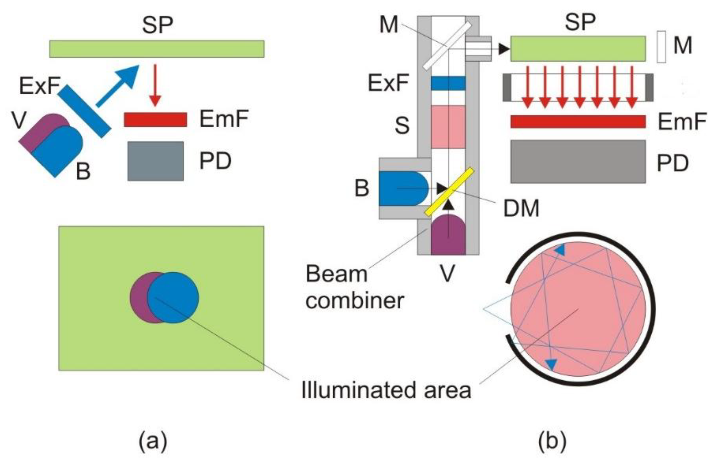
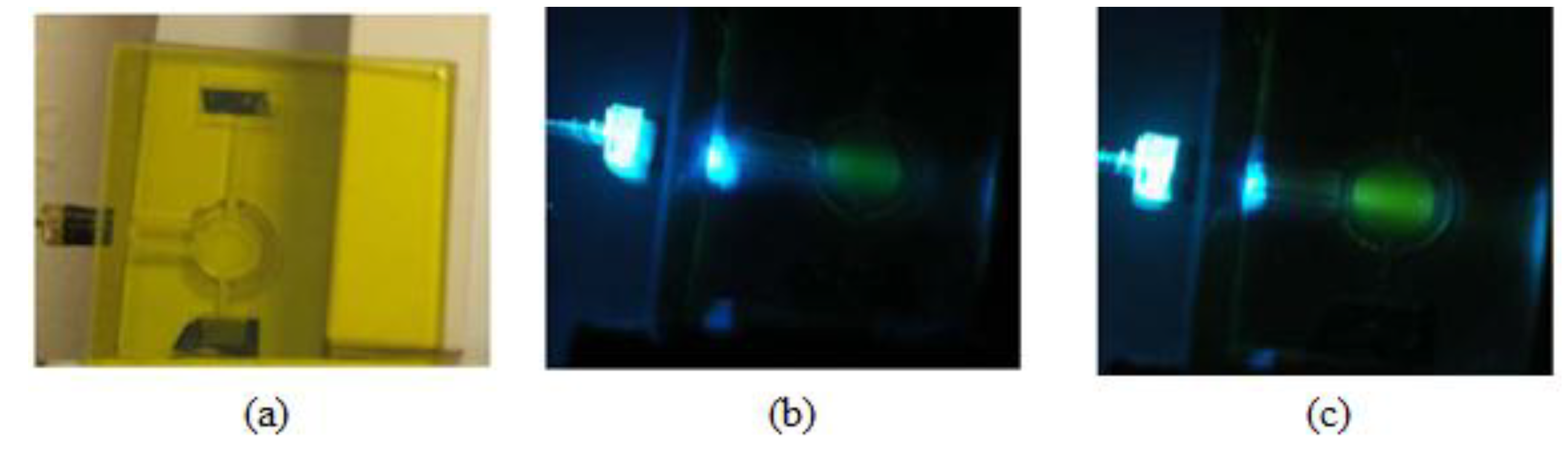
To significantly boost the sensitivity, while preserving the low cost, we used a new sensing scheme shown in Figure 1b. In order to provide more uniform and intense light, a specialized optic device called a beam combiner was developed. Both the blue (Cree, Durham, NC, USA) and violet (Biovar, Irvine, CA, USA) LEDs are mounted inside a block, which also accommodates a dichroic mirror (Andover SP-400). The dichroic mirror transmits the light of the violet LED and reflects the light of the blue LED. Both beams pass through a short pass excitation BG-12 filter (Schott, Mainz, Germany). The beam combiner is also equipped with a 90%/10% splitter (microscope cover glass), which allows 90% of the light to proceed toward the measurement chamber, but directs 10% toward the reference photodiode (S-1223-1, Hamamatsu, Japan; not shown in Figure 1b). In this way, all the optics are housed in a single block, which makes it shock proof and environmentally insensitive. After passing through the short-pass filter, the violet and blue excitations are reflected off a mirror to the side of the measurement chamber, where the CO2-sensitive dye solution is injected. The fluorescence emission is then measured underneath. This 90° separation between excitation and emission minimizes the scattered light that reaches the detector. A dye solution is better than a solid sensor patch in this application, because the former is renewable, and thus, photobleaching, one of the major problems for optical sensors, can be avoided [7,8,9]. The reflective mirror around the measurement chamber increases the capture of the excitation light and the uniform excitation of the dye. Thus, it can significantly increase the fluorescence intensity while not increasing or even lowering the intensity of the scattered light. The photos in Figure 2 provide convincing evidence that this approach will work. The panel on the left is a laser-milled prototype of the measurement chamber. The middle panel shows the blue LED excitation of a fluorescein solution without the reflective mirror, and the final image on the right shows the fluorescence from the mirrored chamber. It can be seen that the fluorescence from the mirrored chamber is much brighter, while the co-planar excitation results in very little blue scattered light normal to the excitation.
2.3. The Design and Construction of More Stable Readout System
Scattered light, one of the major noise sources, was greatly reduced by the novel approach shown in Figure 1b. Except for scattered light, another source of noise is the fluctuations in light source intensity. The LED intensity depends on two factors: the current through the PN junction, as well as the temperature of the junction. As the current through the LED is kept constant by using the negative feedback of the source, the drift of the LED brightness is due to the gradual increase of the junction temperature caused by resistive heating. In theory, it is possible to turn the LED on and wait until it thermally equilibrates. However, this does not prevent ambient thermal drift. The heating decreases the output intensity, which may vary up to 0.1%. As a ratio of the two intensities is being used and the errors in a ratio multiply, the ratio can fluctuate up to 0.4%. This is not adequate for the resolution that we are trying to achieve. Our first attempt to overcome this problem is to introduce analog negative-feedback correction [29]. While it stabilizes the long-term drift, it introduces significant noise in the signal and leads to substantial degradation of the S/N. For this reason, we elected to monitor the LED brightness by adding a reference photodetector and using it to normalize the detected fluorescence intensity. The amplification chains for both detectors were adjusted in such a way that the reference and the sensing signal were roughly the same magnitude, leading to a ratio that exhibited the same sensitivity in both channels.

Figure 2.
Laser-milled measurement chamber (a);blue LED excitation of a fluorescein solution without the reflective mirror (b) and the fluorescence from the mirrored chamber (c).
Figure 2.
Laser-milled measurement chamber (a);blue LED excitation of a fluorescein solution without the reflective mirror (b) and the fluorescence from the mirrored chamber (c).
In addition to the scattered light and drift of LED brightness caused by resistive heating or ambient temperature fluctuation, analog synchronous rectification and averaging are sources of additional noise. As a result, we elected to remove the synchronous rectification switches and the low pass filtering and to implement this functionality in the software. This approach is often termed “software lock-in” and relies on a fast analog to digital converter (ADC). We have selected ADC 8613, a 500 ksps 16-bit successive approximation register ADC, operated twice per period. These measures significantly boosted the instrument performance by more than 10 fold. Of course, the trade-off is the cost, which is approximately doubled in terms of component costs to around $300.
2.4. The Construction of the Microfluidic Chip
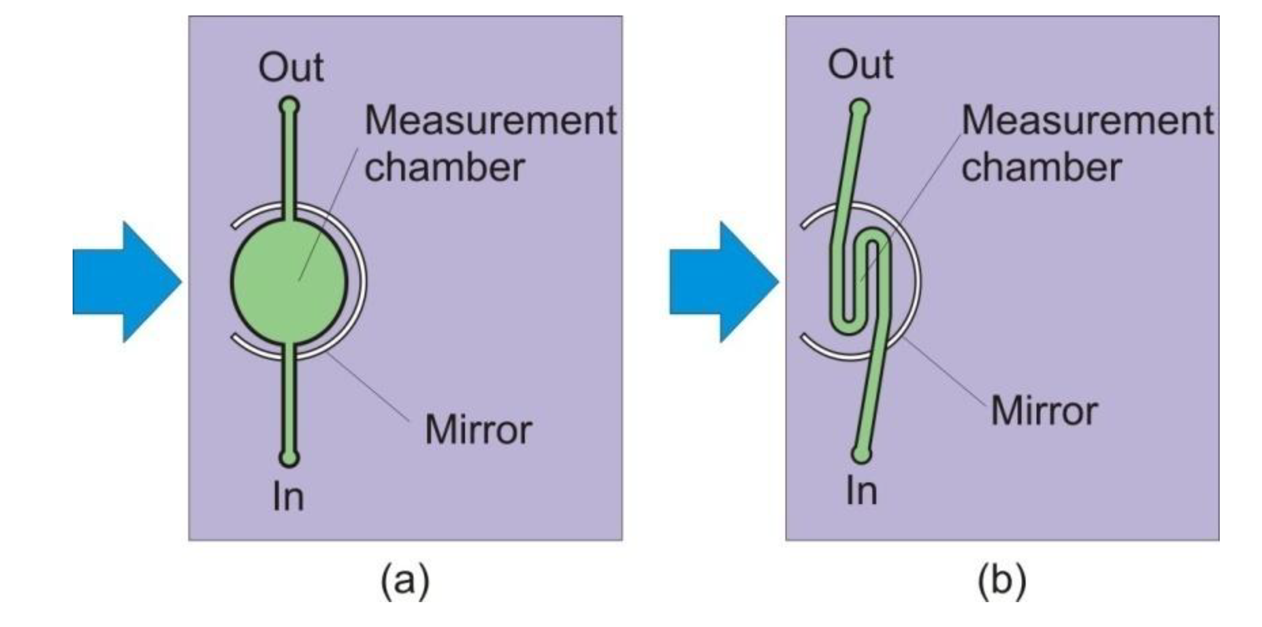
In our first design, the measurement chamber (MC) in Figure 1 is elliptical in shape, as shown in Figure 2 and Figure 3a. To minimize dye retention, the elliptical measurement chamber was replaced by a micro-channel measurement chamber, as shown in Figure 3b. The volume of the measurement chamber was significantly reduced to only 5.0 μL.

Figure 3.
The elliptical measurement chamber (a) in our initial design was replaced by a micro-channel measurement chamber (b); and the volume of the chamber was significantly reduced to only 5.0 µL.
Figure 3.
The elliptical measurement chamber (a) in our initial design was replaced by a micro-channel measurement chamber (b); and the volume of the chamber was significantly reduced to only 5.0 µL.
The microfluidic chip was made of multilayer poly(methyl methacrylate) sheets of different thicknesses (Professional Plastics, Cheektowaga, NY, USA). First, a specific pattern on each sheet was cut with a laser cutter (Universal Laser Systems, Scottsdale, AZ, USA) or a milling machine (Shanghai SIEG Group, Shanghai, China). The sheets were then bonded together. Several bonding techniques, including adhesive bonding with double-sided tape (Adhesives Research, Glen Rock, PA, USA), solvent bonding with chloroform and thermal bonding [30], were tested. Thermal bonding was superior to adhesive or solvent bonding, because the optical and fluorescent properties of the chamber were maintained during construction, and the tiny channel geometries remained intact with minimal distortion or blocking. Dye entrapment at the interface due to the adhesive was also avoided. The chamber made by thermal bonding was capable of >80 psi service without any leaking. It was observed that the optical clarity of the machined channels could be significantly improved by solvent polishing, and annealing the material reduced its internal stress and, thus, could reduce cracks occurring during fabrication or in use. The solvent-assisted thermal bonding procedure used in this research was described in detail elsewhere [31].
Figure 4 shows an assembled detection board, including the electronics board, with USB communication, the beam combiner and the microfluidic chip.
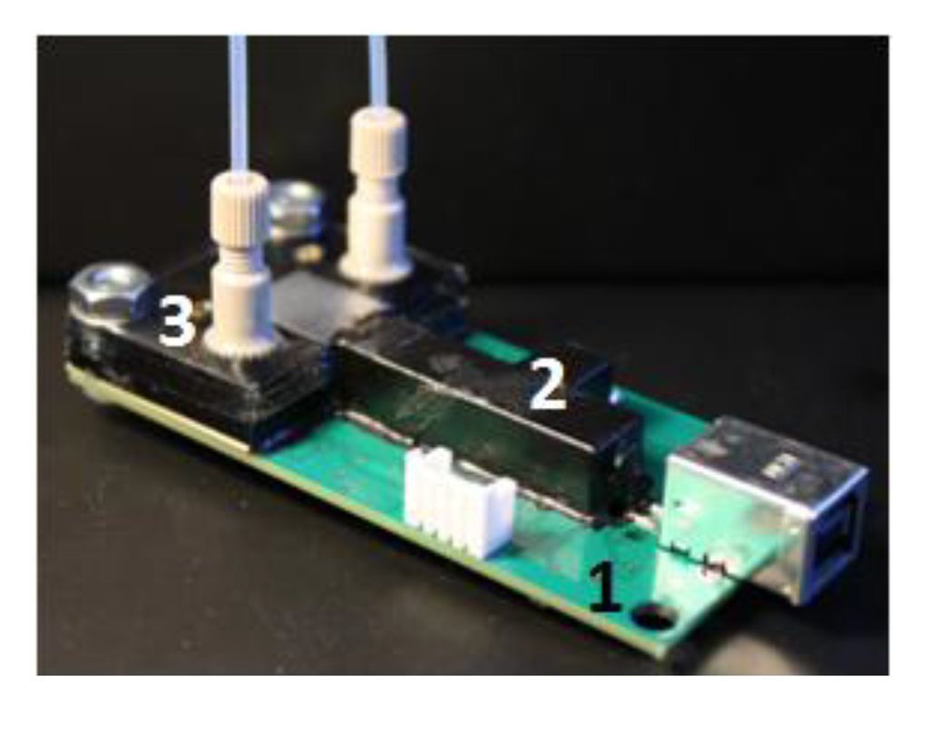
Figure 4.
The assembled detection board with USB communication. 1, electronics board; 2, beam combiner; 3, microfluidic chip.
Figure 4.
The assembled detection board with USB communication. 1, electronics board; 2, beam combiner; 3, microfluidic chip.

2.5. The Test of the System
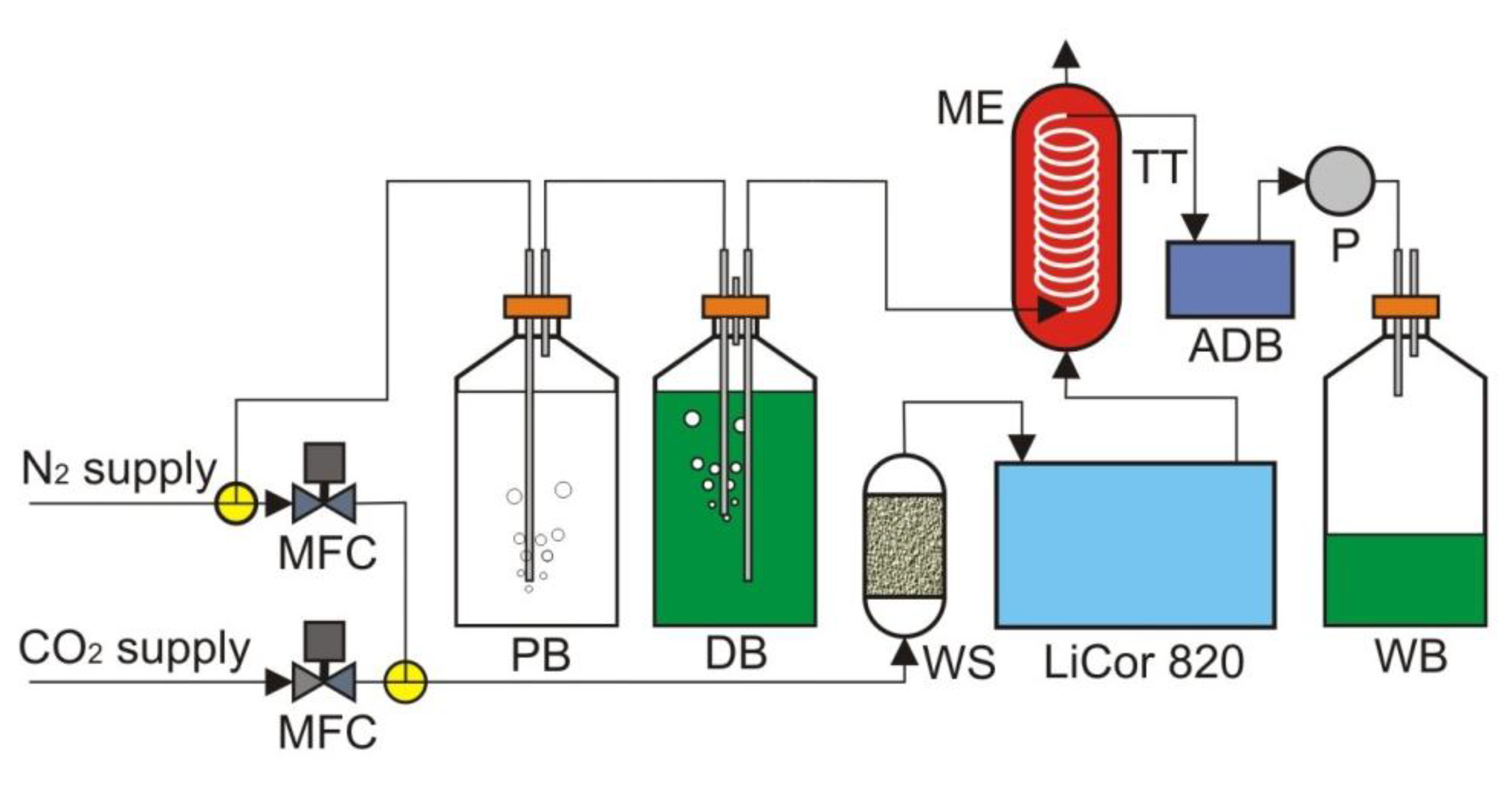
The test setup is shown in Figure 5. Nitrogen from the lab supply was first passed through deionized water before bubbling through the dye solution. Because the gas had a very low moisture content, when it was passed through a liquid, it had the potential to strip moisture out of that liquid. The addition of the pre-saturation bottle helped to mitigate the loss of water and the change in concentration of dye in the following dye bottle. The mass exchanger contained 5 feet of Teflon AF 2400 tubing. Teflon AF 2400 was used as our exchange membrane tubing, due to its exceptional gas permeability. The membrane tubing was wound around a central support structure in such a way that the winding minimized both the contact of the tubing with itself and with the support structure. The assembled detection board with a 5 µL on-chip dye volume was hooked inline between the mass exchanger and a small peristaltic pump. A CO2-free dye was pulled into the Teflon AF 2400 tubing in the mass exchanger, allowed to equilibrate with a flowing gas mixture containing CO2 and then pulled through the detection board by the peristaltic pump to the waste bottle. While the pump was in operation, the detection board was constantly reading the fluorescence ratio of the dye. The flowing gas mixture containing CO2 was produced using two mass flow controllers.
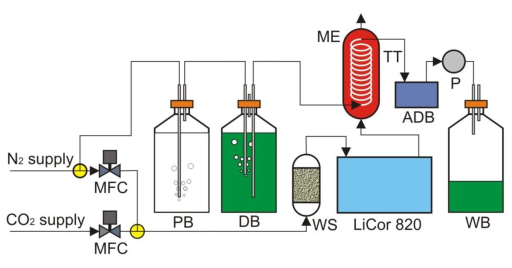
Figure 5.
The test setup. ADB, assembled detection board; DB, dye bottle; ME, mass exchanger; MFC, mass flow controller; P, pump; PB, pre-saturation bottle; TT, Teflon tubing; WB, waste bottle; WS, water scrubber.
Figure 5.
The test setup. ADB, assembled detection board; DB, dye bottle; ME, mass exchanger; MFC, mass flow controller; P, pump; PB, pre-saturation bottle; TT, Teflon tubing; WB, waste bottle; WS, water scrubber.
3. Results and Discussion
We first optimized the sensing reagent formula to find the optimal dye and base concentrations to satisfy the required sensing range. For a diluted dye solution, its fluorescence intensity goes up when its concentration increases. A higher fluorescence intensity gives stronger signals and a higher S/N. However, if the concentration continues to increase beyond a certain point, the inner filtering effect will dominate, and the fluorescence intensity begins to decrease. The optimal dye concentration is such that it has the highest S/N. Measurements conducted in a 3-mL quartz cuvette with a 1-cm optical path length showed that the optimal dye concentration for HPTS was 50 µM. As CO2 is acidic when dissolved in water, an initial basic environment is required for the pH indicator to respond to CO2. At a very low base concentration, the dye solution is very sensitive to low concentrations of CO2, but will be quickly saturated when pCO2 goes up. Higher base concentration can widen the sensing range of the dye solution, but lower its sensitivity. Therefore, the optimal base concentration is such that the dye has the largest signal change when pCO2 changes from 200 µatm to 600 µatm. Tests showed that the optimal base concentration was 20–100 µatm M. To analyze the effect of base concentration on the sensitivity of the detection, mathematical modeling was also performed, which confirmed the experiment results. Other buffering species can lower the sensitivity of the detection and, thus, should be avoided. The working dye solution contains 50 µatm M HPTS, 40 µatm M sodium carbonate and 700 mM NaCl. When the two solutions on both sides of the gas-permeable membrane have different ionic strength, osmotic pressure will force water vapor to diffuse across the membrane and cause the sensor to drift. To minimize any interferences, 700 mM of NaCl was added to the dye solution to match the ionic strength of seawater. Other dyes, like CNF and DHPDS, were also tested. They have similar sensitivity, but HPTS has the highest stability.
The detection board was first tested using a 3-mL quartz cuvette with the above working dye solution. The S/N was calculated to be 1,123:1, more than four times higher than the Varian Fluorescence Spectrophotometer, even though the detection board was built exclusively with low-cost optics and electronics. The response curve of the detection board (Figure 4) to a dye solution equilibrated to a flowing gas stream across a membrane is shown in Figure 6. The lower picture is the response curve of three equilibration cycles at 200 µatm CO2. The top picture shows only the lower part of the response curve of 20 equilibration cycles at different CO2 concentrations. As the detection board read the pulled dye solution stream, the old dye was washed out. The equilibrated dye solution dominated the readings during the plateau phase, and new CO2-free dye was pulled through the detection board before it reached equilibrium in the rising phase. From the same figure, one can see that the dye solution did reach a different equilibrated value at each gas set point.
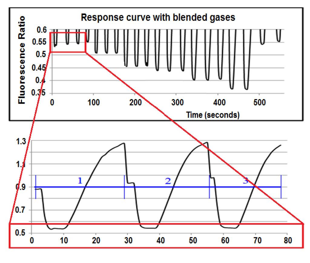
Figure 6.
The response curve of the sensor.
Figure 6.
The response curve of the sensor.

A calibration curve of the fluorescence ratio as a function of the dry gas CO2 fugacity is shown in Figure 7. The square of the correlation coefficient for the power function trend line is close to one, showing that the calibration data can be fitted to the power function very well. The precision at each set point was calculated based on the standard deviation of the three different readings at that point. The precisions at the set points are given in Table 2. It can be seen that the sensor has an average precision of 1.7 µatm pCO2. Although this precision is still lower than the best currently available sensor for pCO2 in seawater, which is about 1 µatm, it is a good result, taking into consideration the small size and low cost of the described system. Measures to further improve the performance of the system are under investigation.

Figure 7.
The calibration curve of the fluorescence intensity ratio vs. the dry gas CO2 fugacity. The error bars are the standard deviation of triplicate measurements.
Figure 7.
The calibration curve of the fluorescence intensity ratio vs. the dry gas CO2 fugacity. The error bars are the standard deviation of triplicate measurements.
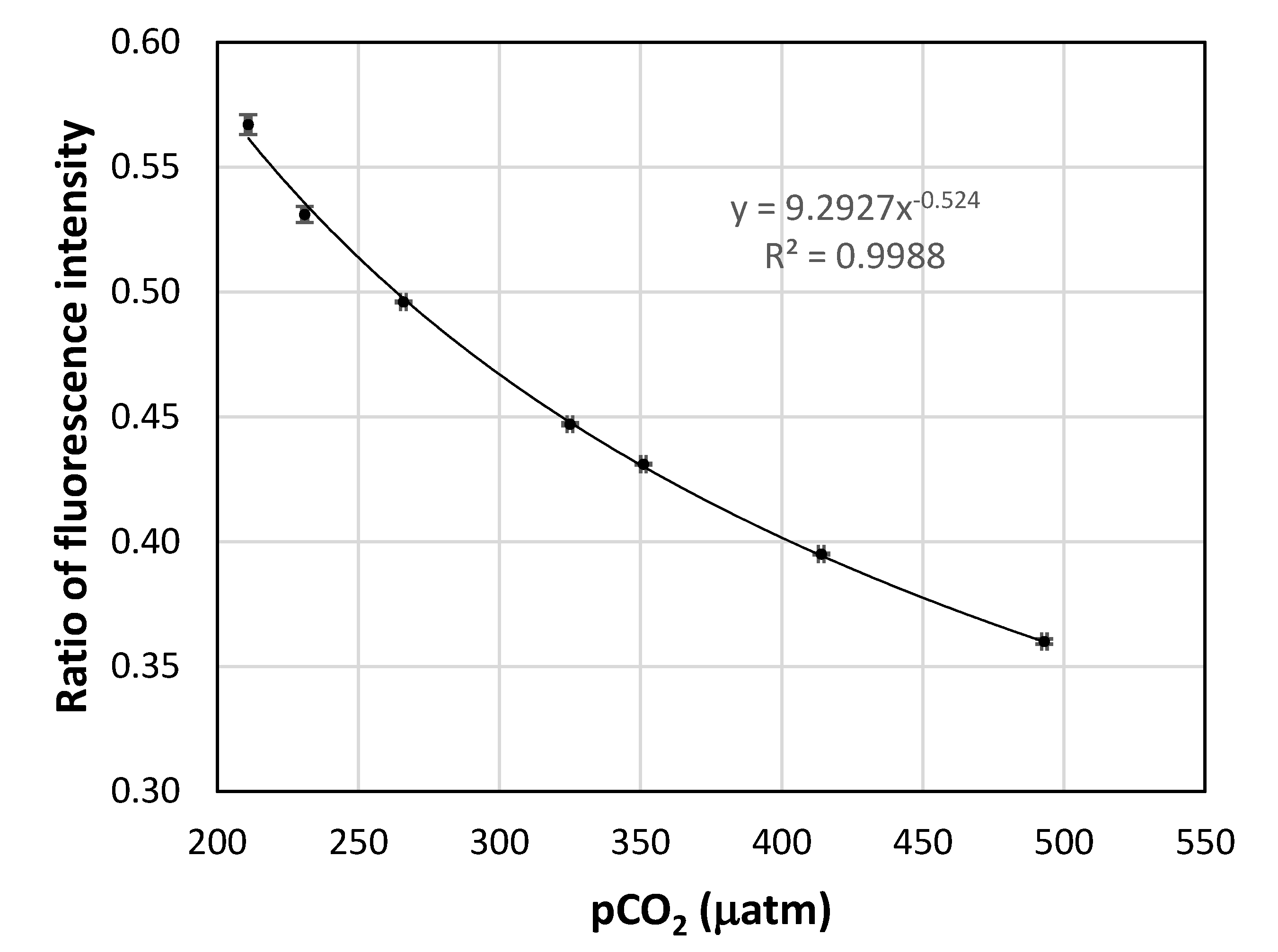
Table 2.
Sensor precision at different set points.
| Set Point (µatm) | Precision (µatm) |
|---|---|
| 211 | ±3.6 |
| 231 | ±3.2 |
| 266 | ±0.4 |
| 325 | ±1.1 |
| 351 | ±0.7 |
| 414 | ±0.8 |
| 493 | ±2.4 |
| Average | ±1.7 |
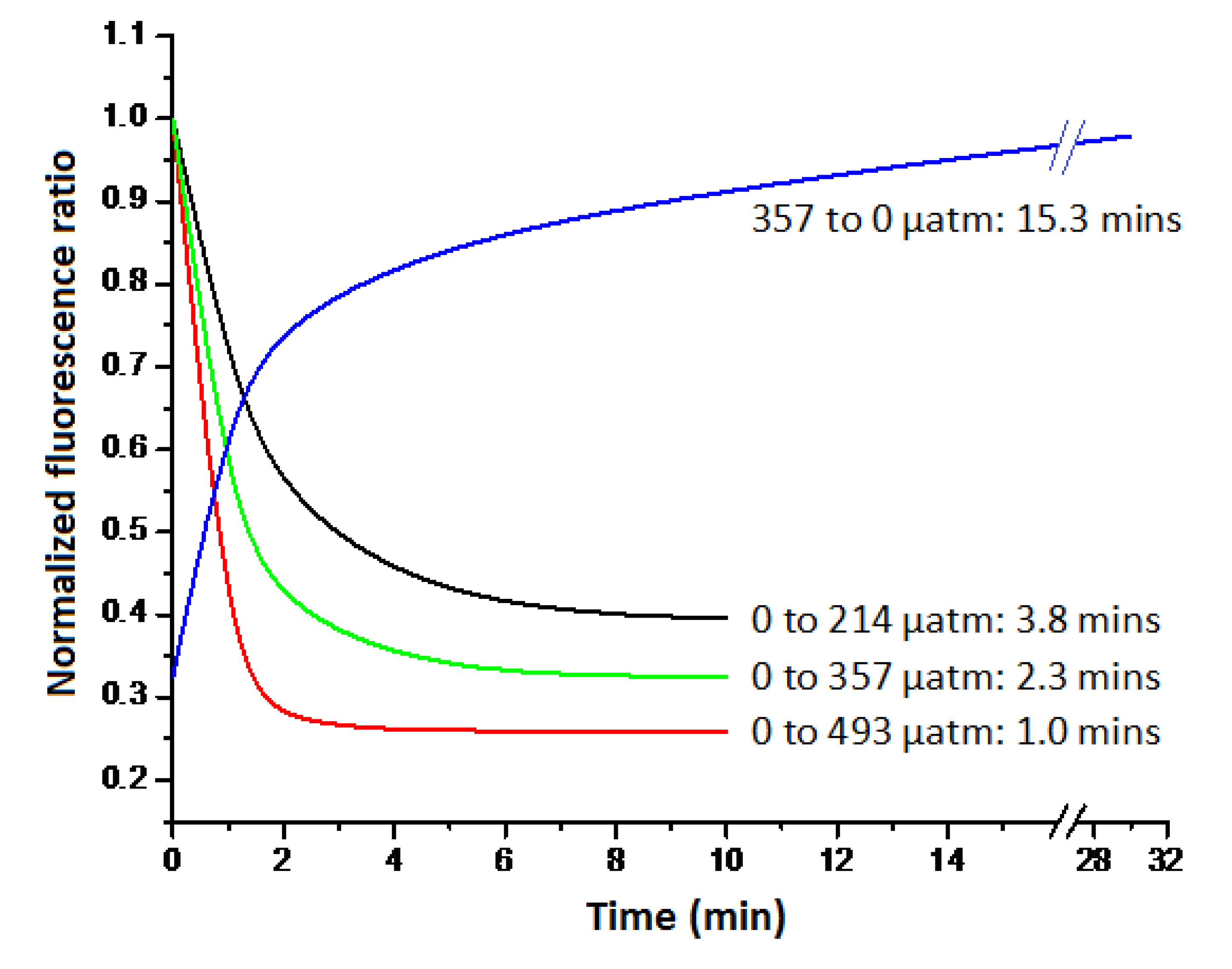
The response time of the sensor to step changes in CO2 fugacity is very rapid, due to the nature of the Teflon AF 2400 membrane tubing and the small geometries involved. The response curves of the sensor to step changes in CO2 fugacity are shown in Figure 8. The 90% response time of a CO2-free dye to a gas phase on the other side with a CO2 fugacity of 214, 357 or 493 µatm is only 1.0, 2.3 and 3.8 min, respectively. It can be seen that the larger the step change in pCO2, the faster the response time. Finally, when a dye is used to measure the fugacity of CO2 across the membrane, the dye kept in its basic state responds to changes in CO2 concentrations more readily. This effect is noted in Figure 8. It is apparent that a change of the same magnitude, from zero to 357 µatm CO2 or from 357 back to 0 µatm CO2, takes a considerably different amount of time. Therefore, from the point of view of response time, it is better to keep the dye solution in a CO2-free or a low CO2 state.

Figure 8.
The responses of the sensor to different step changes in CO2 fugacity.
Figure 8.
The responses of the sensor to different step changes in CO2 fugacity.
4. Conclusions
A low-cost fluorescent sensor for measurements of pCO2 was built. The sensor was exclusively assembled with low-cost optics and electronics. The total cost of the system is less than $1,000, so it is affordable enough to be deployed in great numbers. Several performance-boosting strategies were used in the sensor development, including the 90° separation between excitation and emission, the beam combiner, the reference photodetector, etc. Initial tests showed that the sensor is stable and fast. It can achieve an average resolution of 1.7 µatm, despite the low cost. Further improvement on the precision requires the tuning of the system, which is being investigated.
Acknowledgments
This research is funded by the Office of Naval Research, Award Number N00014-10-1-0243.
Author Contributions
All authors contributed to this work. X.G. built the initial microfluidic chip and wrote the main paper. Y.K. designed and built the electronics and wrote part of the Experimental Section. R.H. and N.S. modified the microfluidic chip, built the experimental setup and performed the experiments. G.R. supervised the project and edited the manuscript. All authors contributed to the data analysis.
Conflict of Interest
The authors declare no conflict of interest.
References
- Doney, S.C.; Anderson, R.; Bishop, J.; Caldeira, K.; Carlson, C.; Car, M.E.; Feely, R.; Hood, M.; Hopkinson, C.; Jahnke, R.; et al. Ocean. Carbon and Climate Change (OCCC): An Implementation Strategy for U.S. Ocean. Carbon Research; UCAR: Boulder, CO, USA, 2004. [Google Scholar]
- Kleypas, J.A.; Feely, R.A.; Fabry, V.J.; Langdon, C.; Sabine, C.L.; Robbins, L.L. Impacts of Ocean. Acidification on Coral Reefs and Other Marine Calcifiers. A Guide for Future Research. Report of a workshop sponsored by NSF, NOAA and the USGS: St. Petersburg, FL, USA, 18–20 April 2005. [Google Scholar]
- Mayhew, P.J.; Jenkins, G.B.; Benton, T.G. A long-term association between global temperature and biodiversity, origination and extinction in the fossil record. Proc. Biol. Sci. 2008, 275, 47–53. [Google Scholar] [CrossRef]
- Solomon, S.; Plattner, G.K.; Knutti, R.; Friedlingstein, P. Irreversible climate change due to carbon dioxide emissions. Proc. Natl. Acad. Sci. USA 2009, 106, 1704–1709. [Google Scholar] [CrossRef]
- Walt, D.R.; Gabor, G. Multiple-indicator fiber-optic sensor for high-resolution pCO2 sea water measurements. Anal. Chim. Acta 1993, 274, 47–52. [Google Scholar] [CrossRef]
- Tabacco, M.B.; Uttamlal, M.; McAllister, M.; Walt, D.R. An autonomous sensor and telemetry system for low-level pCO2 measurements in seawater. Anal. Chem. 1999, 71, 154–161. [Google Scholar] [CrossRef]
- DeGrandpre, M.D. Measurement of seawater pCO2 using a renewable-reagent fiber optic sensor with colorimetric detection. Anal. Chem. 1993, 65, 331–337. [Google Scholar] [CrossRef]
- DeGrandpre, M.D.; Hammar, T.R.; Smith, S.P.; Sayles, F.L. In situ measurements of seawater pCO2. Limnol. Oceanogr. 1995, 40, 969–975. [Google Scholar] [CrossRef]
- DeGrandpre, M.D.; Baehr, M.M.; Hammar, T.R. Calibration-free Optical chemical sensors. Anal. Chem. 1999, 71, 1152–1159. [Google Scholar] [CrossRef]
- Wolfbeis, O.S.; Kovacs, B.; Goswami, K.; Klainer, S.M. Fiber-optic fluorescence carbon dioxide sensor for environmental monitoring. Mikrochim. Acta 1998, 129, 181–188. [Google Scholar] [CrossRef]
- Neurauter, G.; Klimant, I.; Wolfbeis, O.S. Fiber-optic microsensor for high resolution pCO2 sensing in marine environment. Fresenius J. Anal. Chem. 2000, 366, 481–487. [Google Scholar] [CrossRef]
- Wang, Z.A.; Liu, X.; Byrne, R.H.; Wanninkhof, R.; Bernstein, R.E.; Kaltenbacher, E.A.; Pattern, J. Simultaneous spectrophotometric flow-through measurements of pH, carbon dioxide fugacity, and total inorganic carbon in seawater. Anal. Chim. Acta 2007, 596, 23–36. [Google Scholar] [CrossRef]
- Hanson, M.A.; Ge, X.; Kostov, Y.; Brorson, K.A.; Moreira, A.R.; Rao, G. Comparisons of Optical pH and Dissolved Oxygen Sensors with Traditional Electrochemical Probes during Mammalian Cell Culture. Biotechnol. Bioeng. 2007, 97, 833–841. [Google Scholar] [CrossRef]
- Ge, X.; Hanson, M.; Kostov, Y.; Moreira, A.R.; Rao, G. Validation of an optical sensor-based high-throughput bioreactor system for mammalian cell culture. J. Biotechnol. 2006, 122, 293–306. [Google Scholar] [CrossRef]
- Ge, X.; Kostov, Y.; Rao, G. Low-cost noninvasive optical CO2 sensing system for fermentation and cell culture. Biotechnol. Bioeng. 2005, 89, 329–334. [Google Scholar] [CrossRef]
- Ge, X.; Kostov, Y.; Rao, G. High-Stability Non-Invasive Autoclavable Naked Optical CO2 Sensor. Biosens. Bioelectron. 2003, 18, 857–865. [Google Scholar] [CrossRef]
- Kermis, H.R.; Kostov, Y.; Harms, P.; Rao, G. Dual excitation ratiometric fluorescent pH sensor for noninvasive bioprocess monitoring: development and application. Biotechnol. Prog. 2002, 18, 1047–1053. [Google Scholar] [CrossRef]
- Kermis, H.R.; Kostov, Y.; Rao, G. Rapid method for the preparation of a robust optical pH sensor. Analyst 2003, 128, 1181–1186. [Google Scholar] [CrossRef]
- Kostov, Y.; Harms, P.; Pilato, R.S.; Rao, G. Ratiometric oxygen sensing: Detection of dual-emission ratio through a single emission filter. Analyst 2000, 125, 1175–1178. [Google Scholar]
- Harms, P.; Kostov, Y.; Rao, G. Bioprocess monitoring. Curr. Opin. Biotechnol. 2002, 13, 124–127. [Google Scholar] [CrossRef]
- Tolosa, L.; Kostov, Y.; Harms, P.; Rao, G. Noninvasive measurement of dissolved oxygen in shake flasks. Biotechnol. Bioeng. 2002, 80, 594–597. [Google Scholar] [CrossRef]
- Gryczynski, Z.; Rao, G. Polarization oxygen sensor: A template for a class of fluorescence-based sensors. Anal. Chem. 2002, 74, 2167–2171. [Google Scholar] [CrossRef]
- Bambot, S.; Sipior, J.; Lakowicz, J.R.; Rao, G. Lifetime-Based Optical Sensing of pH Using Resonance Energy Transfer in Sol-Gel Sensors. Sens. Actuatos B 1995, 22, 181–188. [Google Scholar]
- Sipior, J.; Bambot, S.; Romauld, M.; Carter, G.M.; Lakowicz, J.R.; Rao, G. A Lifetime-Based Optical CO2 Gas Sensor with Blue or Red Excitation and Stokes or Anti-Stokes Detection. Anal. Biochem. 1995, 227, 309–318. [Google Scholar] [CrossRef]
- Holavanahali, R.; Romauld, M.; Carter, G.M.; Rao, G.; Sipior, J.; Lakowicz, J.R.; Bierlein, J. A Directly-Modulated Diode Laser Frequency-Doubled in a KTP Waveguide as an Excitation Source for CO2 and O2 Phase Fluorometric Sensors. J. Biomed. Opt. 1996, 1, 124–130. [Google Scholar] [CrossRef]
- Yuan, S.; DeGrandpre, M.D. A comparison between two detection systems for fiber optic chemical sensor applications. Appl. Spectrosc. 2006, 60, 465–470. [Google Scholar] [CrossRef]
- Wang, Z.; Wang, Y.; Cai, W.J.; Liu, S.Y. A long pathlength spectrophotometric pCO2 sensor using a gas-permeable liquid-core waveguide. Talanta 2002, 57, 69–80. [Google Scholar]
- US Department of Energy. Handbook of Methods for the Analysis of the Various Parameters of the Carbon Dioxide System in Sea Water, 2nd ed.; Dickson, A.G., Goyet, C., Eds.; US Department of Energy: Washington, DC, USA, 1994; ORNL/CDIAC-74. [Google Scholar]
- Palma, A.J.; Ortigosa, J.M.; Lapresta-Fernandez, A.; Fernandez-Ramos, M.D.; Carvajal, M.A.; Capitan-Vallvey, L.F. Portable light-emitting diode-based photometer with one-shot optochemical sensors for measurement in the field. Rev. Sci. Instrum. 2008, 79, 103–105. [Google Scholar]
- Brown, L.; Koerner, T.; Horton, J.H.; Oleschuk, R.D. Fabrication and characterization of poly(methylmethacrylate) microfluidic devices bonded using surface modifications and solvents. Lab. Chip 2006, 6, 66–73. [Google Scholar] [CrossRef]
- Henderson, R.M.; Selock, N.; Rao, G. Robust and easy microfluidic connections in acrylic. Chips and Tips. 2012. Available online: http://blogs.rsc.org/chipsandtips/2012/04/23/robust-and-easy-macrofluidic-connections-in-acrylic/ (accessed on 27 March 2014).
© 2014 by the authors; licensee MDPI, Basel, Switzerland. This article is an open access article distributed under the terms and conditions of the Creative Commons Attribution license (http://creativecommons.org/licenses/by/3.0/).