Abstract
The resonant frequency of an SAW oscillator can be modulated by varying the signal amplitude, due to non-linear acoustic interactions within the chemoselective layer. In this study, we developed an explicit model to describe the amplitude–frequency behavior of a tunable SAW oscillator. A polymeric layer of variable thickness was deposited in a circular area (radius 1.1 mm) at the center of the piezoactive surface. Increasing the oscillator loop attenuation resulted in a continuous increase in the resonant frequency by up to 1.8 MHz. The layer was modeled as a succession of non-interacting sub-layers of varying thicknesses. As a result, the function model consists of a superposition of terms, each corresponding to a layer region of distinct length and thickness. The maximum difference between the experimental data and function model (also known as residual of the fit) was below 1% (13.02 kHz) of the resonant frequency variation, thus supporting the validity of our approach. While our model proved successful, the results suggest that some interactions are unaccounted for, as evidenced by the periodicity of the residuals of fit and unrealistically large variation in acoustic wave velocity.
1. Introduction
The continuous expansion of human civilization has led to a growing demand for sensing devices that are accurate, affordable, and high-performing—a trend that shows no signs of slowing down. This demand pertains not only to quantity but also to quality. As an example, a complex air chemical composition assessment is needed for the food industry as a means to evaluate the state of perishable food items. In addition, due to the continuous industrial development, environmental pollution has become ubiquitous, posing a problem even in indoor domestic spaces [1]. This is because a plethora of complex chemical compounds is slowly released into the air by furniture and domestic appliances, and many of them are a health hazard even in low concentrations [2]. Air toxins such as formaldehyde, acetaldehyde, 1,4-dichlorobenzene, chloroform, carbon tetrachloride, benzene, and naphthalene have been identified as pollutants of potential concern because of several risk-based analyses [3,4]. Multiple disorders associated with VOC indoor air pollution were amply reported, such as irritation of the eyes and nose, respiratory dysfunctions, sick-building syndrome, and leukemia, especially in children [5,6,7,8,9,10,11,12,13]. As a result, the specialized literature abounds in reports on new developments in this field, most reporting advances in the field of materials used for chemoselective layers. An important aspect limiting the SAW (surface acoustic wave) sensors’ success is the complex interactions governing their functionality, some of which are related to device-layer acoustic interactions. Still, it is due to this complexity that SAW devices are a natural option for complex environmental and material assessment. Sustained efforts have been made to harness the inherent complexity of these acoustic devices. The design and implementation of multi-mode/multi-frequency SAW devices have also been tested for the integration of the functionality of an entire sensor array into one single device. This approach consists of designing an SAW device capable of generating different modes simultaneously [14], multiple-order resonance [15], and both multi-mode and multi-frequency responses [16]. In the same vein, an interesting approach was to probe wavefront scattering by using multiple receiving IDTs [17]. Device-layer acoustic interaction is the basis of our approach to expanding the acoustic wave sensor’s capability. Resonant frequency variation due to non-linear reactions in a chemoselective layer within an SAW loop oscillator has the potential to greatly expand the application area of SAW devices. This technique works best in combination with soft polymeric chemoselective layers. However, proper calibration of the device is necessary in order to extract valid sensing information. Until now, this has proved a difficult task, due to the technique’s sensitivity to the slightest differences in layer morphology. Therefore, the analytical information contained in the SAW sensor’s amplitude–frequency characteristic must be deconvoluted from the effects of the morphological features of the layer. Developing an explicit functional model for the layer reaction would allow for the quantification of its physical properties and therefore account for their changes. Such a model could then be used to calibrate SAW sensors in spite of the differences in the morphology of their chemoselective layers, and it could serve as a foundation for an analytical protocol based on a single SAW sensor. This perspective becomes even more promising in light of recent insights [18] into the physics of SAW propagation, which suggest the potential for implementing hypersensitive SAW sensors using this technique. In our previous article [19], the effect of layer morphology and position on the amplitude–frequency characteristics of a tunable SAW oscillator was qualitatively evaluated. One important result was that the frequency trend appeared to be almost linearly dependent on attenuation. This behavior of the resonant frequency rendered our previous model [20] unusable for the characteristics tested in [19], presumably due to its limited generality. In [20], the layer covers nearly the entire piezoactive area; in the second case, over 90% of it remains exposed. For this type of layer, we propose a new model that accounts for the general case in which the layer partially covers the SAW device and successfully fits the experimental data.
2. Materials and Methods
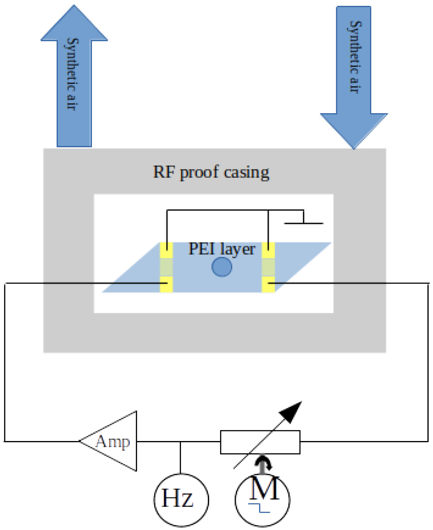
The tunable oscillator consists of an SAW device with a central frequency of 70 MHz connected in a closed-loop configuration with a DHPVA-200 FEMTO amplifier (Messtechnik GmbH, Berlin, Germany). The SAW sensor consists of an ST-X cut quartz substrate with interdigital transducers (IDTs) made of 200 nm thick gold electrodes deposited on a 10 nm chromium adhesion layer, patterned using standard photolithography. A double/double finger design was employed, featuring 50 electrode pairs with a periodicity of 11 µm, resulting in a resonant frequency of approximately 69 MHz. A potentiometer included in the oscillator’s feedback loop allowed resonant frequency control, via non-linear acoustic reaction of the PEI (Polyethylenimine) layer deposited on the SAW device. The SAW was placed in an RF-isolated, closed chamber filled with synthetic air with zero humidity. On the center of the SAW device, a roughly circular, 2.2 mm diameter PEI layer was deposited. This was created by drop casting a 0.2 L 1% by weight PEI solution in ethanol. Visual inspection revealed that the PEI film resulting after solvent evaporation had random variations in thickness, with the thickest point being located close to the center of the layer. Signal attenuation in the feedback loop influences the effective amplitude at the SAW surface, thereby modulating the non-linear response of the polymer layer. Changing the resonant frequency of the SAW oscillator was possible using a rotary potentiometer inserted into the feedback loop. A computer-controlled, high-precision, motorized rotary stage was used to actuate the potentiometer, thus providing fast, precise, and fine-grained frequency control. For maintaining stable experimental conditions, the SAW device was placed on a 87 Watt Peltier element which maintained a constant temperature of 25 ± 0.1 °C. Automated, real-time temperature adjustment was made by a TEC-1089 Meerstetter Peltier controller. A schematic of the setup is presented in Figure 1.

Figure 1.
Experimental setup for the tunable SAW oscillator.
A CNT-90-type frequency counter (Spectracom Corp, Rochester, NY, USA) was used to acquire the resonant frequency values. Custom-made software automated the entire measurement process, consisting of successive potentiometer actuations and frequency data acquisition.
3. Modeling
The most prominent methods for addressing the problem under study are parametric non-linear regression and the finite element method (FEM). Although FEM is a powerful and widely used simulation tool, it presents significant challenges in this context. At the operating frequency (∼60 MHz), FEM requires an extremely fine mesh to accurately resolve wave propagation across the millimeter-scale geometry of the device, resulting in prohibitively high computational demands. Furthermore, the non-linear viscoelastic behavior of the polymer layer is difficult to parameterize due to the lack of precise higher-order material constants. To address a more general case than that of uniform coverage, the polymeric layer in our configuration was intentionally deposited in a localized shape, covering only a portion of the piezoactive SAW region. Additionally, due to the nature of the deposition technique, the layer’s shape was irregular in both contour and thickness. This kind of partial and asymmetric coverage further complicates any FEM-based simulation, as it would require detailed spatial characterization and fine spatial meshing—conditions that are rarely practical in experimental setups. By contrast, the parametric analytical model we developed accounts for such interactions in a simplified yet physically meaningful way. It enables efficient evaluation without the need for fine spatial meshing or exhaustive material data. Moreover, the model captures the non-linear behavior of the polymer layer through fitted parameters, making it well suited for non-linear regression with experimental data.
In an SAW oscillator, the central resonant frequency is the result of interdigital transducers’ spatial frequency and acoustic wave propagation velocity. Besides that, the resonant frequency must fulfill the standing wave condition, i.e., the acoustic and electric path length all across the oscillators loop amounts to an integer number of wavelengths. Depositing a layer on the SAW surface increases the inertia of the material that undergoes acoustic oscillations. With a constant imparted oscillatory energy, the conservation law dictates a reduction in surface wave propagation velocity and wavelength. As a result, the resonant frequency of the oscillator will shift so that it regains the standing wave condition, adjusting for the wavelength reduction due to a decrease in velocity. Also, in an acoustically thick layer, the top surface shear oscillation lags behind the oscillation at the layer–SAW interface. In other words, the shear oscillation reflected by the top surface of the layer exhibits a significant phase difference with respect to the shear waves of the piezoelectric surface. The interference between the two shear waves results in the wavefront at the SAW surface being delayed or advanced, resulting in either a decrease or an increase in wave propagation velocity and a subsequent resonant frequency adjustment. The two effects briefly outlined above are called gravimetric and acoustic effects, and they are both accounted for by the following equation [21]:
where = and . In the above equations, v is the surface wave propagation velocity, Im() represents the imaginary part of the expression, index j gives the oscillation’s polarization, i is the imaginary unit, is the SAW–film coupling parameter [21], tanh() is the hyperbolic tangent function, is the wave pulsation 2πf with f being the oscillation frequency of the SAW, is the surface acoustic wave velocity of an uncoated SAW, is the layer density, and . In this model, phase difference = Re(ih), where Re() represents the real part of the expression in parenthesis.
We will approximate the layer as a succession of m adjacent sub-layers of different lengths (k = 1…m), with constant thicknesses (see Figure 2). Under our experimental conditions, the number of sub-layers yielding the best fit was eleven (m = 11). In the general case, the layer does not cover the entire piezoactive area, so a length of the free SAW surface will be included, where L is the distance between the two IDTs. Accordingly, we approximate the total time T needed for the wavefront to cross the space between the two IDTs as the sum of the times required to traverse all the sub-layers, plus the time needed to cross the uncovered portion of the SAW surface. The total wavefront propagation time is therefore given by
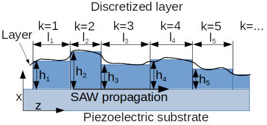
Figure 2.
PEI layer decomposition in sub-layers.
Considering the standing wave condition, the total propagation time is equal to an integer number of wave periods, i.e., T = n, where n is an integer and is the wave period. By substituting wave period with resonant frequency f in Equation (2), we obtain
For the chemoselective layer, we preferred a polymer, for its pronounced non-linear response. Shear thinning is specific to polymeric materials, and consists of viscosity reduction proportional to the shear rate. In our setup, the SAW oscillator resonant frequency shift due to amplitude variation is the effect of the loss coefficient G″ dependence on the oscillation amplitude, i.e., shear thinning [22,23]. For the purposes of this study, both the argument and the scaling factor of the hyperbolic tangent function in Equation (1) are approximated using first-degree complex polynomials in attenuation x. For each oscillation polarization, an independent set of parameters is provided. To alleviate the departure from the non-linearity of the original formula and to account for the differences between them, distinct parameters will be used for the argument and the scaling factor of the hyperbolic tangent function. In addition to varying the purely complex part, we will introduce parameters and to account for non-linear effects in the purely real part of the expressions, thereby enhancing the model’s flexibility. Thus, the multiplicative factor of the tangent function will be represented by a variable complex quantity, with a linear dependence on the signal attenuation x, . This quantity is polarization-mode-specific (indexed by j) in Equation (1), resulting in three sets of parameters. As mentioned, we opted for an independent expression for the argument of the hyperbolic tangent, also with distinct parameters for each oscillation mode j. Due to the energy amount dissipated along the way, the oscillatory amplitude varies across sub-layer locations. This is due to the attenuation of acoustic energy during wave propagation, which leads to a spatially varying amplitude profile. Thus, a parameter will be provided to scale the attenuation x accordingly, with its value constrained within the [0, 1] interval. Although this choice may seem counterintuitive—since attenuation increases with propagation and one might expect a scaling factor greater than 1—it is important to note that part of the attenuation effect is implicitly included in other multiplicative terms such as , , and . Therefore, the [0, 1] range for is effectively equivalent to a higher-than-unity range. We adopted this formulation to enhance computational efficiency. Considering all of the above, the velocity , corresponding to a portion of the sub-layer of thickness , can be written as follows:
The final form of the model used for data fitting is obtained by substituting Equation (4) into Equation (3) and carrying out the summation over eleven sub-layers, indexed from k = 1 to 11.
The goodness of fit will be quantified based on the coefficient of determination (R2) and the maximum of absolute fit residual. The coefficient of determination gives a measure of how close the response function is to experimental results. It is given by subtracting the ratio between the residual sum of squares and the total sum of function response squares from unity. It takes values between 1 and 0, and it reaches unity in the ideal case of perfect fit, i.e., the residual sum of squares is null. Measurement units were normalized to centimeters and seconds by constants and L, with values of 1.4 × cm/s and 1 cm, respectively. Constraints were imposed on sub-layer lengths and thicknesses, such that 0, 0, and 0.22 cm. Additionally, the number of wavelentghs n, corresponding to resonant standing wave mode, was constrained to the interval [150, 200]. All other parameters were left unconstrained.
4. Results
The amplitude–frequency dependence of the SAW oscillator was probed for 245 different attenuation values. Its profile closely resembles those presented in (20) and consists of an increasing resonant frequency from 59.5 MHz to well above 60 MHz. It is characterized by the presence of two sigmoids and a significant number of curvatures and sharp, small-scale variations. Also, an overall slight curvature of the frequency variation can be noted.
We used the NonlinearModelFit function in Wolfram Mathematica to perform the parameter estimation. The model, as defined by Equations (3) and (4), was provided as input along with the corresponding experimental resonance frequencies. The fitting procedure was based on a least-squares minimization of the differences between experimental and theoretical resonance frequencies, returning both the optimal parameters and the goodness-of-fit metrics. Fitting attempts were made for different numbers of component sub-layers. By successive testing, the optimal number of component sub-layers was established to eleven (k = 1 to 11), the optimization criteria being the maximization of the coefficient of determination (R2). In Figure 3, the fitting model and residuals are presented side by side.
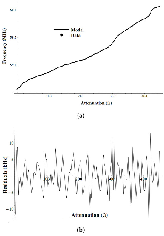
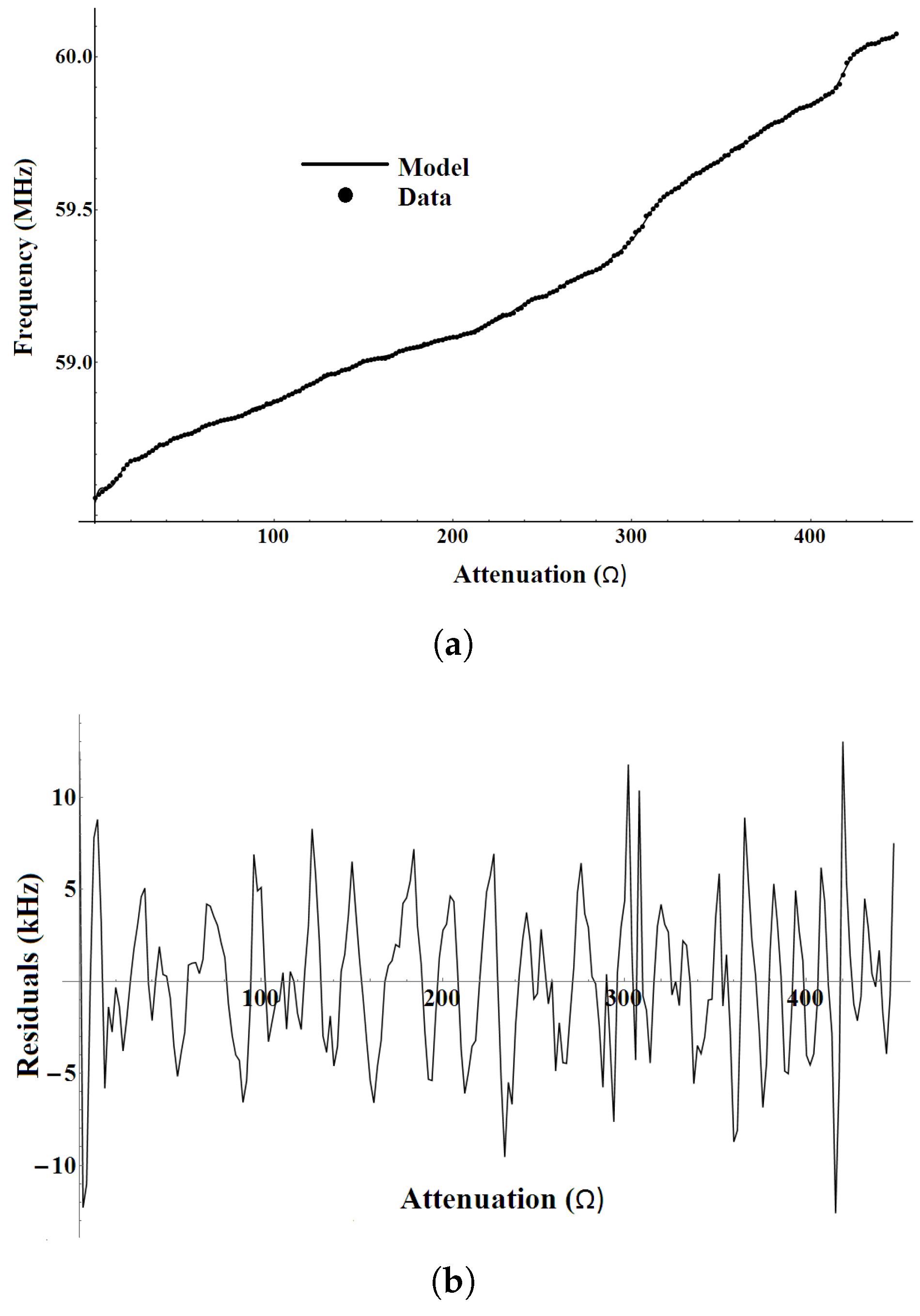
Figure 3.
(a) Model fit and experimental data. (b) Fit residuals.
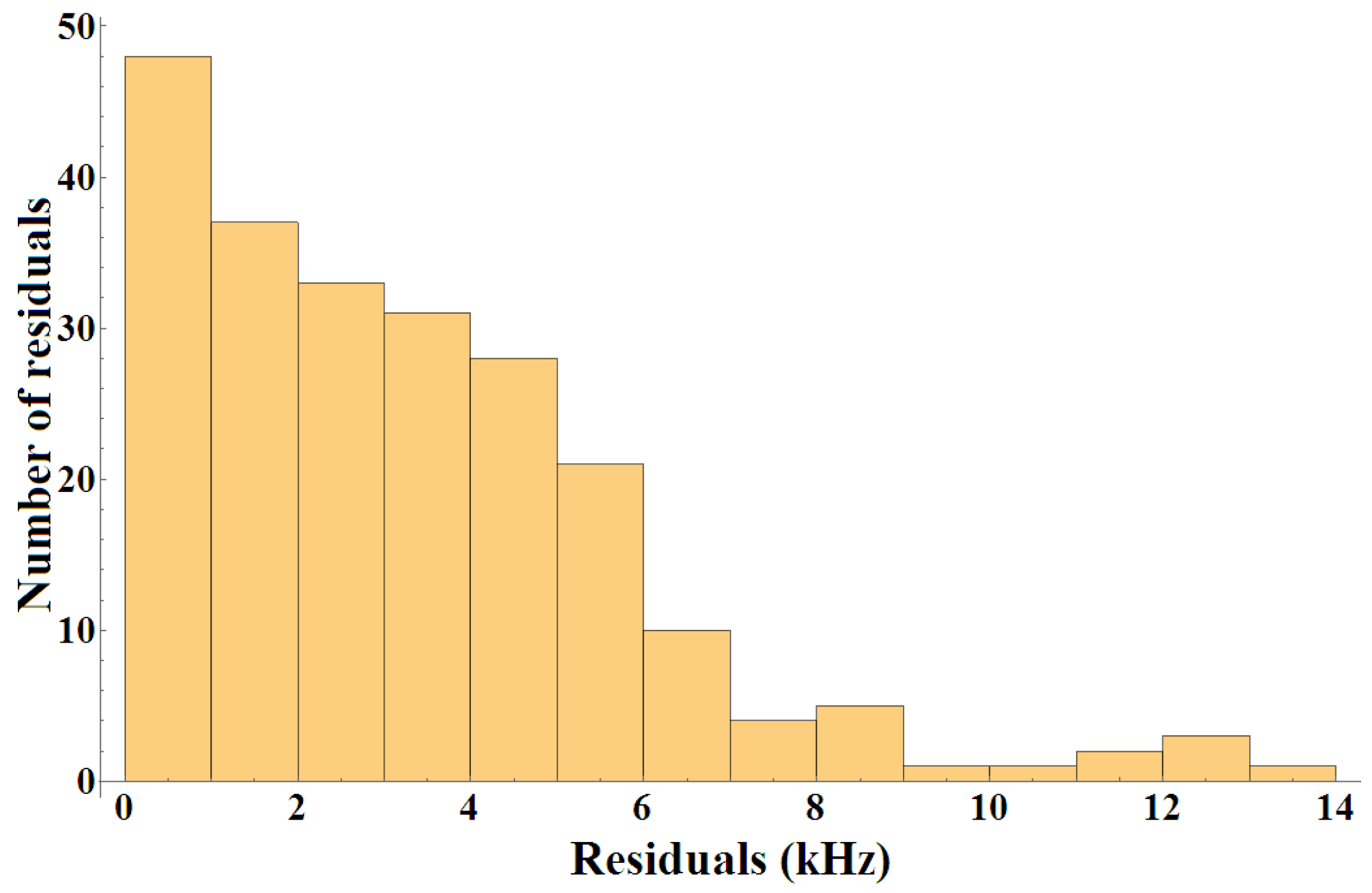
The graphical representation of the model fit versus experimental data in Figure 3 demonstrates the excellent agreement between the model and the measurements. This is also confirmed by the coefficient of determination (), which has a value of more than 0.99997, only marginally less than unity. This value signifies exceptional accuracy of the proposed model. While the large number of parameters certainly played a role, it is still a strong indication that the theoretical reasoning behind the model appears well founded. Additionally, Figure 4 shows the residual histogram. While the maximum residual was 13.020 kHz, the vast majority of residuals were below 7 kHz, and more than 50% of them fell below 5 kHz.
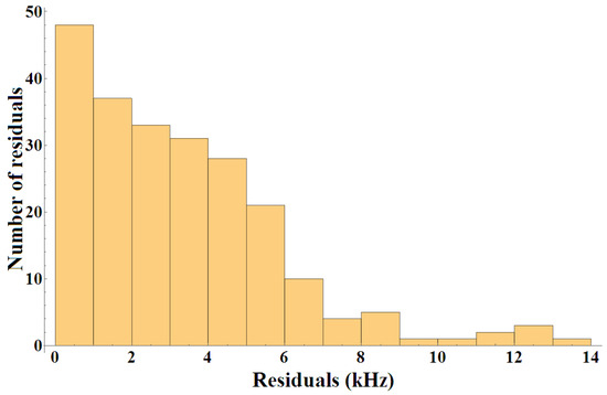
Figure 4.
Histogram of residuals.
As shown in Figure 3, the variation in fit residuals exhibits a discernible oscillatory pattern. A clear peak–valley alternation is observable, which contrasts with the expected random distribution originating from stochastic processes and suggests a systematic origin for the model–data discrepancies. One possible explanation could be unaccounted wave interference between adjacent sub-layers of differing thicknesses. This hypothesis is strongly supported by the periodic nature of the residuals.
In Table 1, oscillation mode (j)-related and sub-layer (k)-related parameters are given. The number of wavelengths, n, is 150.52. The parameters associated with the elasticity module (B and BB) are small, two and three orders of magnitude lower, respectively. Although this may be expected, they are non-zero and contribute partially to amplitude–frequency characteristics. Moreover, it is not necessary to tie its origin to the SAW device, since it could be caused by complex amplification and measurement electronics. This hypothesis can be readily tested, as a detection experiment involving analytes should leave their values unchanged. We emphasize that parameters do not represent sub-layer thicknesses, as they are part of the multiplicative factor within the argument of the hyperbolic tangent function. While, in principle, they could offer a relative measure of sub-layer thicknesses, this is also not the case, due to the implicit approximation of the layer as a PEI strip transverse to the wave propagation direction. It remains to be experimentally tested if their values are valid indicators that could be used in a detection/identification protocol. The lengths , on the other hand, have their units fixed due to the presence of the constants L and in Equation (2), though they are still presumably affected by the approximation of the layer as a transverse strip. Nevertheless, their behavior may provide valuable insights into the model’s limitations. Additionally, it is possible that, even without direct physical significance, they might still function as valid indicators in a detection protocol.

Table 1.
Parameter values. Top: Oscillation mode parameters. Bottom: Sub-layer component parameters.
5. Discussion
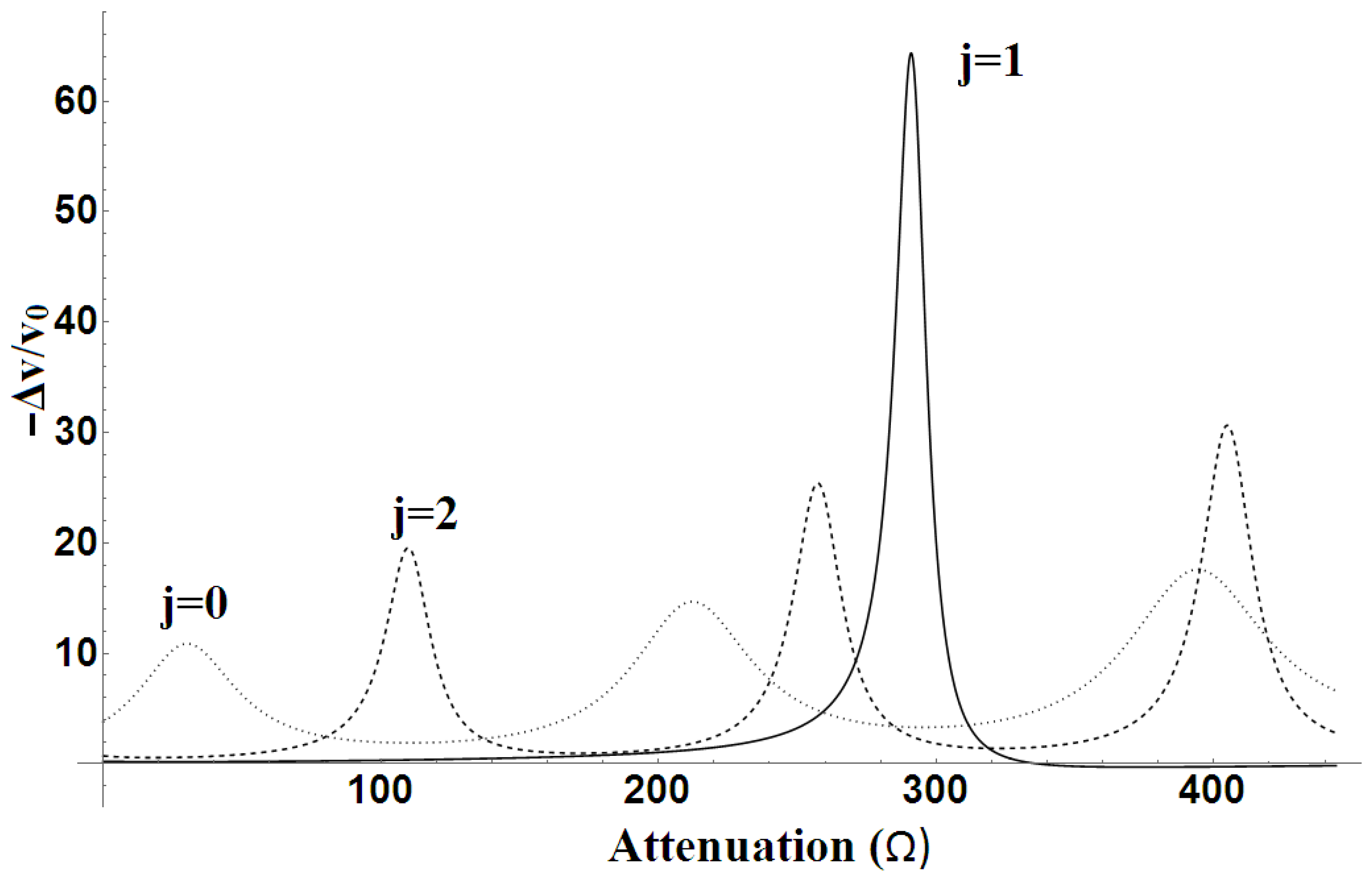
Separate plotting of the relative velocity variation brings unexpected high values to attention, such as the one seen in Figure 5. For comparison purposes, the fitting procedure was also performed using a different model (not included here), featuring a smaller number of components ( to 6) and independent parameter sets (A to ) for each sub-layer, totaling 61 parameters. Although the fitting criteria were acceptable—with a maximum residual of 17.8 kHz—the resulting relative velocity variation was even higher, reaching several hundred. This strongly suggests that the elevated relative velocity values result from the lower number of components. In such a case, high-amplitude/high-frequency components become necessary to reproduce the fine details of the amplitude–frequency profile. Furthermore, the unrealistic propagation velocity excursions might stem from the unaccounted non-linearity in both the hyperbolic tangent argument and its multiplying factor.
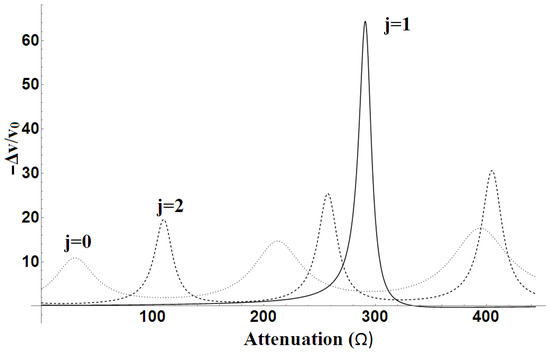
Figure 5.
Relative velocity variation for the sub-layer k = 4.
While the magnitude of the velocity variation might suggest that the oscillatory modes in the model correspond to the x, y, and z polarizations of the acoustic waves, the presence of the PEI layer complicates this interpretation. Z-polarized modes correspond to compression waves, and the large value of the bulk modulus E typically suppresses such resonances. Therefore, it is plausible that the observed resonances are artifacts arising from layer discretization and the limited number of sub-layer components. This interpretation is further reinforced by the presence of multiple-layer resonances.
Although the finite element method (FEM) is a powerful general-purpose simulation tool, it is not well suited for this specific problem. At the operating frequency (60 MHz), FEM requires an extremely fine mesh to resolve wave behavior over the millimeter-scale geometry, resulting in prohibitively large computational loads. Additionally, the non-linear viscoelastic behavior of the polymer layer is difficult to parameterize for FEM because accurate higher-order material constants are unavailable. By contrast, our analytical model captures the non-linearity through fitted parameters and can be evaluated quickly, without the burden of meshing or detailed material data.
In a conventional configuration—where the chemoselective layer covers the entire piezoactive surface—higher-order resonances are highly unlikely due to the strong energy dissipation in viscoelastic polymer films [21]. However, when the layer covers only a small portion of the surface, the dissipated energy is proportionally reduced. This leads to a lower effective loss modulus and, in turn, allows for higher propagation velocity excursions and potentially multiple-layer resonances. At this stage, the precise origin of the modeled relative velocity behavior remains unclear. Another anomaly is the relatively low number of wave cycles, around 150. By comparison, the number of wavelengths corresponding to the uncovered length of the SAW surface at a 60 MHz resonant frequency is 152. This mismatch can be attributed to the anomalously high wave velocity—an effect clearly shown in Figure 4. Again, this supports the hypothesis that the model’s limited number of sub-layers fails to fully capture the actual physical profile of the deposited film. In reality, the PEI layer is not composed of discrete sub-layers but rather exhibits a continuous thickness gradient. A more accurate modeling strategy would involve integrating the propagation velocity across a layer with a continuously varying thickness. Provided that such an approach is mathematically and computationally viable, it represents the intended next step in our model development. On the other hand, significant velocity variations may indeed be required to account for the observed resonance excursion. To better understand this, one should examine Equation (3), where the denominator consists of the total time required for the wavefront to pass through both the covered and uncovered regions of the SAW device. For fixed values of , the time needed to cross the uncovered portion is constant—approximately 0.8/(1.4 × 105) cm/s. Since the resonant frequency is inversely proportional to this total propagation time, the magnitude of the velocity variation is amplified by the ratio between the lengths of the covered and uncovered regions. A smaller covered area (as is the case here) necessitates a larger apparent velocity variation to achieve the same total frequency shift. Thus, the high velocity variation seen in the results might be a necessary consequence of the small surface area of the PEI layer. Nevertheless, even if such variation is mathematically consistent, it is not physically plausible that it arises solely from the interactions modeled by Equation (1). This strongly suggests the presence of additional significant interactions. One such factor may be the acoustic lensing effect caused by the circular geometry of the polymer layer. In this configuration, the layer focuses the incident SAW wavefront, resulting in overlapping waves with differing phases. The resulting interference introduces additional velocity modulation that is not explicitly modeled in Equation (1) and is thus erroneously attributed to the modeled interactions, leading to artificially high velocity values.
6. Conclusions
While the model successfully captured the complex amplitude–frequency characteristics, several key questions remain open. Firstly, the issue of the unexpectedly large variations in propagation velocity is one of them. One of the primary goals of this study was to develop a model with a high degree of generality, which led to a relatively complex experimental and modeling scenario. Future investigations should aim to simplify the experimental setup and reduce the number of model parameters, thereby increasing the robustness and interpretability of the results. It is worth noting that the use of the corresponding expressions derived in Equation (1) yielded no meaningful results in this particular context. From a modeling standpoint, the implementation of a continuous variation in layer thickness is likely to be the most beneficial next step. When combined with polymeric layers that fully cover the piezoactive region, this approach would enable a more accurate estimation of acoustic wave velocity variations. Moreover, by fully covering the piezoactive area, the modeling process becomes less dependent on the exact geometry of the deposited layer. Nevertheless, this approach may still prove useful in representing transversal thickness gradients, though its effectiveness may be limited by the fact that the SAW wavefront expands laterally as it approaches the receiving interdigital transducer (IDT). As a result, only a narrow region of the layer directly influences wave propagation. Finally, an important concern remains: the potential utility of this model in the design and implementation of detection or identification protocols for multiple analytes. Targeted experiments will be developed and carried out to address this question and assess the model’s practical applicability in real-world sensing scenarios.
Author Contributions
Conceptualization, I.N.; methodology, I.N.; formal analysis, I.N.; investigation, I.N.; resources, C.V.; writing—original draft preparation, I.N.; writing—review and editing, I.N. and C.V. All authors have read and agreed to the published version of the manuscript.
Funding
This research was supported (or financed) by the Romanian Ministry of Research, Innovation and Digitalization under the Romanian National Nucleus Program LAPLAS VII, with contract no. 30N/2023 and POCIDIF nr. 390008/27.11.2024.
Institutional Review Board Statement
Not applicable.
Informed Consent Statement
Not applicable.
Data Availability Statement
The data presented in this study are available on request from the corresponding author due to legal reasons.
Conflicts of Interest
The authors declare no conflicts of interest.
References
- Missia, D.A.; Demetriou, E.; Michael, N.; Tolis, E.I.; Bartzis, J.G. Indoor exposure from building materials: A field study. Atmos. Environ. 2010, 44, 4388–4395. [Google Scholar] [CrossRef]
- Air Pollution: Current and Future Challenges. EPA-United States Environmental Protection Agency. Available online: https://www.epa.gov/clean-air-act-overview/air-pollution-current-and-future-challenges (accessed on 23 August 2024).
- Loh, M.M.; Levy, J.I.; Spengler, J.D.; Houseman, E.A.; Bennett, D.H. Ranking Cancer Risks of Organic Hazardous Air Pollutants in the United States. Environ. Health Perspect. 2007, 115, 1160–1168. [Google Scholar] [CrossRef] [PubMed]
- Jia, C.; D’Souza, J.; Batterman, S. Distributions of personal VOC exposures: A population-based analysis. Environ. Int. 2008, 34, 922–931. [Google Scholar] [CrossRef] [PubMed]
- Norbäck, D.; Björnsson, E.; Janson, C.; Widström, J.; Boman, G. Asthmatic symptoms and volatile organic compounds, formaldehyde, and carbon dioxide in dwellings. Ocupational Environ. Med. 1995, 52, 388–395. [Google Scholar] [CrossRef] [PubMed]
- Daisey, J.M.; Angell, W.J.; Apte, M.G. Indoor air quality, ventilation and health symptoms in schools: An analysis of existing information. Indoor Air 2003, 13, 53–64. [Google Scholar] [CrossRef] [PubMed]
- Rumchev, K.; Spickett, J.; Bulsara, M.; Phillips, M.; Stick, S. Association of domestic exposure to volatile organic compounds with asthma in young children. Thorax 2004, 59, 746–751. [Google Scholar] [CrossRef] [PubMed]
- Vanos, J.K.; Hebbern, C.; Cakma, S. Risk assessment for cardiovascular and respiratory mortality due to air pollution and synoptic meteorology in 10 Canadian cities. Environ. Pollut. 2013, 185, 322–332. [Google Scholar] [CrossRef] [PubMed]
- Gao, Y.; Zhang, Y.; Kamijima, M.; Sakai, K.; Khalequzzaman, M.; Nakajima, T.; Shi, R.; Wang, X.; Chen, D.; Ji, X.; et al. Quantitative assessments of indoor air pollution and the risk of childhood acute leukemia in Shangha. Environ. Pollut. 2014, 187, 81–89. [Google Scholar] [CrossRef]
- Gonzalez-Flesca, N.; Bates, M.S.; Delmas, V.; Cocheo, V. Benzene exposure assessment at indoor, outdoor and personal levels. Environ. Monit. Asses. 2000, 65, 59–67. [Google Scholar] [CrossRef]
- Salthammer, T.; Mentese, S.; Marutzky, R. Formaldehyde in the indoor environment. Chem. Rev. 2010, 110, 2536–2572. [Google Scholar] [CrossRef] [PubMed]
- Nielsen, G.D.; Wolkoff, P. Cancer effects of formaldehyde: A proposal for an indoor air guideline value. Arch. Toxicol. 2010, 84, 423–446. [Google Scholar] [CrossRef] [PubMed]
- Panagopoulos, I.K.; Karayannis, A.N.; Kassomenos, P.; Aravossis, K. A CFD simulation study of VOC and formaldehyde indoor air pollution dispersion in an apartment as part of an indoor pollution management plan. Aerosol Air Qual. Res. 2011, 11, 758–762. [Google Scholar] [CrossRef]
- Lamanna, L.; Rizzi, F.; Bhethanabotla, V.R.; De Vittorio, M. GHz AlN-based multiple mode SAW temperature sensor fabricated on PEN substrate. Sens. Act. A 2020, 315, 112268. [Google Scholar] [CrossRef]
- Schmalz, J.; Kittmann, A.; Durdaut, P.; Spetzler, B.; Faupel, F.; Höft, M.; Quandt, E.; Gerken, M. Multi-Mode Love-Wave SAW Magnetic-Field Sensors. Sensors 2020, 20, 3421. [Google Scholar] [CrossRef] [PubMed]
- Seidel, W.; Hesjedal, T. Multimode and multifrequency gigahertz surface acoustic wave sensors. Appl. Phys. Lett. 2004, 84, 1407–1409. [Google Scholar] [CrossRef]
- Pamwani, L.; Habib, A.; Melandsø, F.; Ahluwalia, B.S.; Shelke, A. Single-Input and Multiple-Output Surface Acoustic Wave Sensing for Damage Quantification in Piezoelectric Sensors. Sensors 2017, 18, 67. [Google Scholar] [CrossRef] [PubMed]
- Hamdaoui, M. Uncertainty Propagation and Global Sensitivity Analysis of a Surface Acoustic Wave Gas Sensor Using Finite Elements and Sparse Polynomial Chaos Expansions. Vibration 2023, 6, 610–624. [Google Scholar] [CrossRef]
- Nicolae, I.; Bojan, M.; Viespe, C. Acoustic Effects of Uneven Polymeric Layers on Tunable SAW Oscillator. Processes 2024, 12, 1217. [Google Scholar] [CrossRef]
- Nicolae, I.; Viespe, C.; Miu, D.; Marcu, A. Analyte discrimination by SAW sensor variable loop amplification probing. Sens. Actuators B Chem. 2022, 358, 131493. [Google Scholar] [CrossRef]
- Martin, S.J.; Frye, G.C.; Senturia, S.D. Dynamics and response of polymer-coated surface acoustic wave devices: Effect of viscoelastic properties and film resonance. Anal. Chem. 1994, 66, 2201–2219. [Google Scholar] [CrossRef]
- Shaw, M.T.; MacKnight, W.J. Introduction to Polymer Viscoelasticity, 3rd ed.; John Wiley & Sons: Hoboken, NJ, USA, 2005; pp. 25–27. [Google Scholar]
- Ferry, J.D. Viscoelastic Properties of Polymers, 3rd ed.; John Wiley & Sons: New York, NY, USA, 1980; pp. 51–52. [Google Scholar]

Disclaimer/Publisher’s Note: The statements, opinions and data contained in all publications are solely those of the individual author(s) and contributor(s) and not of MDPI and/or the editor(s). MDPI and/or the editor(s) disclaim responsibility for any injury to people or property resulting from any ideas, methods, instructions or products referred to in the content. |
© 2025 by the authors. Licensee MDPI, Basel, Switzerland. This article is an open access article distributed under the terms and conditions of the Creative Commons Attribution (CC BY) license (https://creativecommons.org/licenses/by/4.0/).