Figure 1.
Study workflow outlining the sequential stages from data acquisition through preprocessing, model development, evaluation, interpretability analysis, and deployment.
Figure 1.
Study workflow outlining the sequential stages from data acquisition through preprocessing, model development, evaluation, interpretability analysis, and deployment.
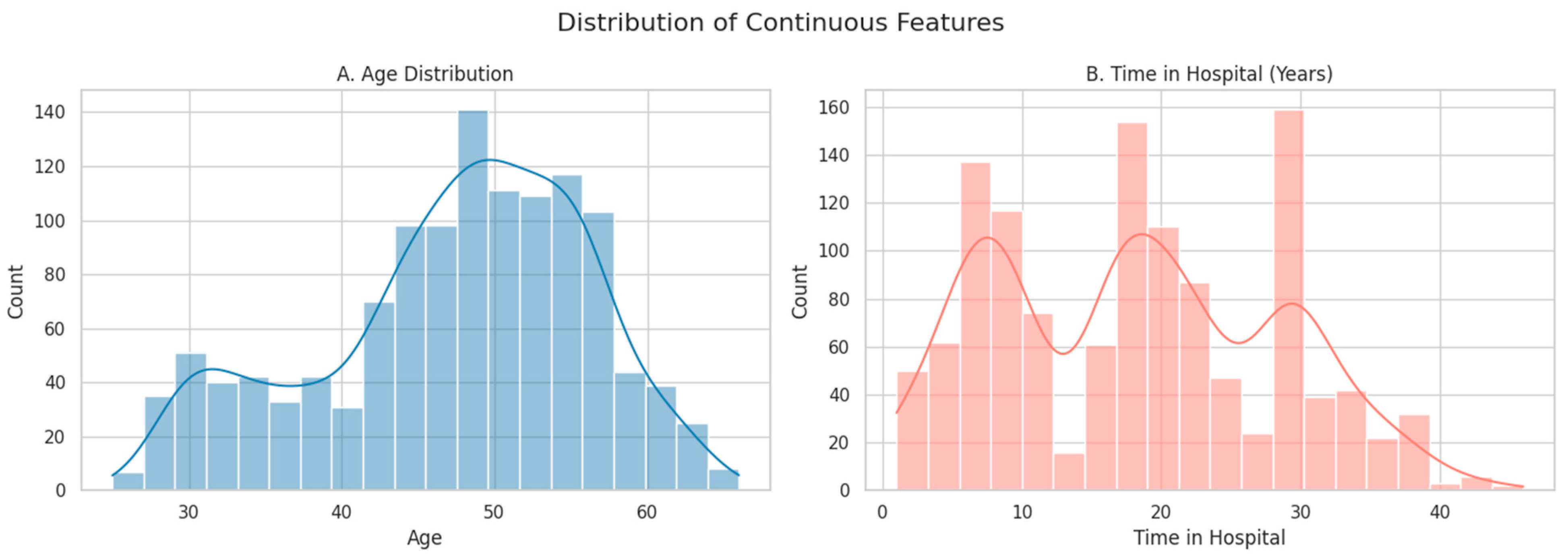
Figure 2.
Histograms showing the distribution of continuous features: (A) Age and (B) Time in Hospital (years). Smooth lines represent kernel density estimates (KDE), which provide a continuous approximation of the underlying distributions.
Figure 2.
Histograms showing the distribution of continuous features: (A) Age and (B) Time in Hospital (years). Smooth lines represent kernel density estimates (KDE), which provide a continuous approximation of the underlying distributions.
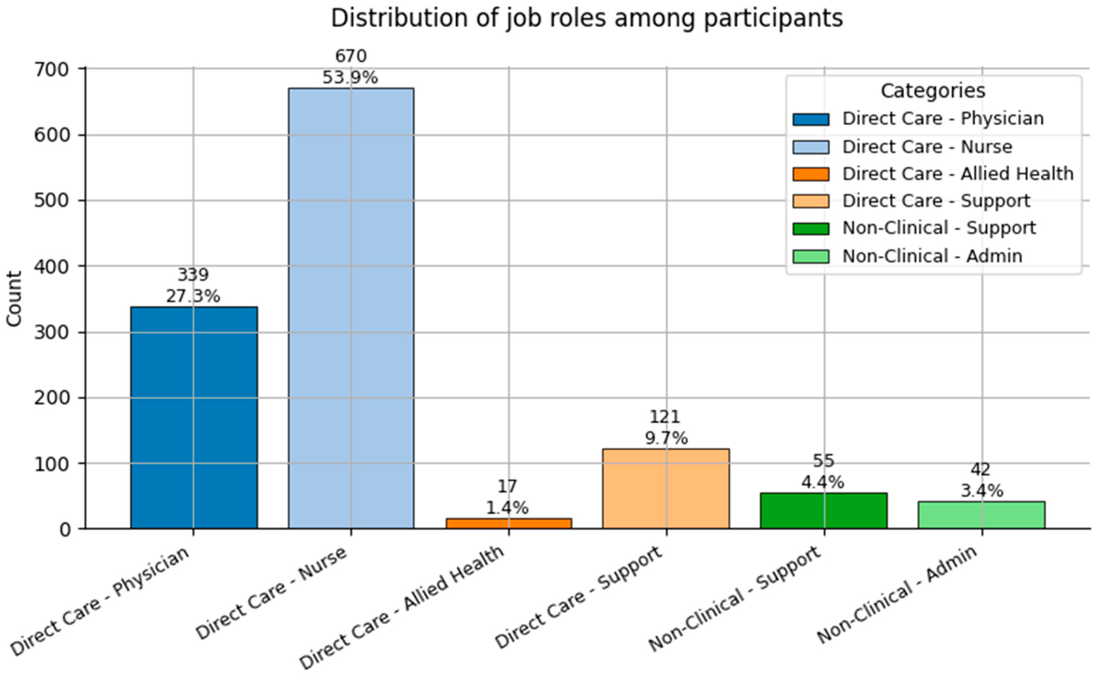
Figure 3.
Distribution of Job Role categories (0 = Direct Care—Physician; 1 = Direct Care—Nurse; 2 = Direct Care—Allied Health; 3 = Direct Care—Support; 4 = Non-Clinical—Support; and 5 = Non-Clinical—Admin) among participants.
Figure 3.
Distribution of Job Role categories (0 = Direct Care—Physician; 1 = Direct Care—Nurse; 2 = Direct Care—Allied Health; 3 = Direct Care—Support; 4 = Non-Clinical—Support; and 5 = Non-Clinical—Admin) among participants.
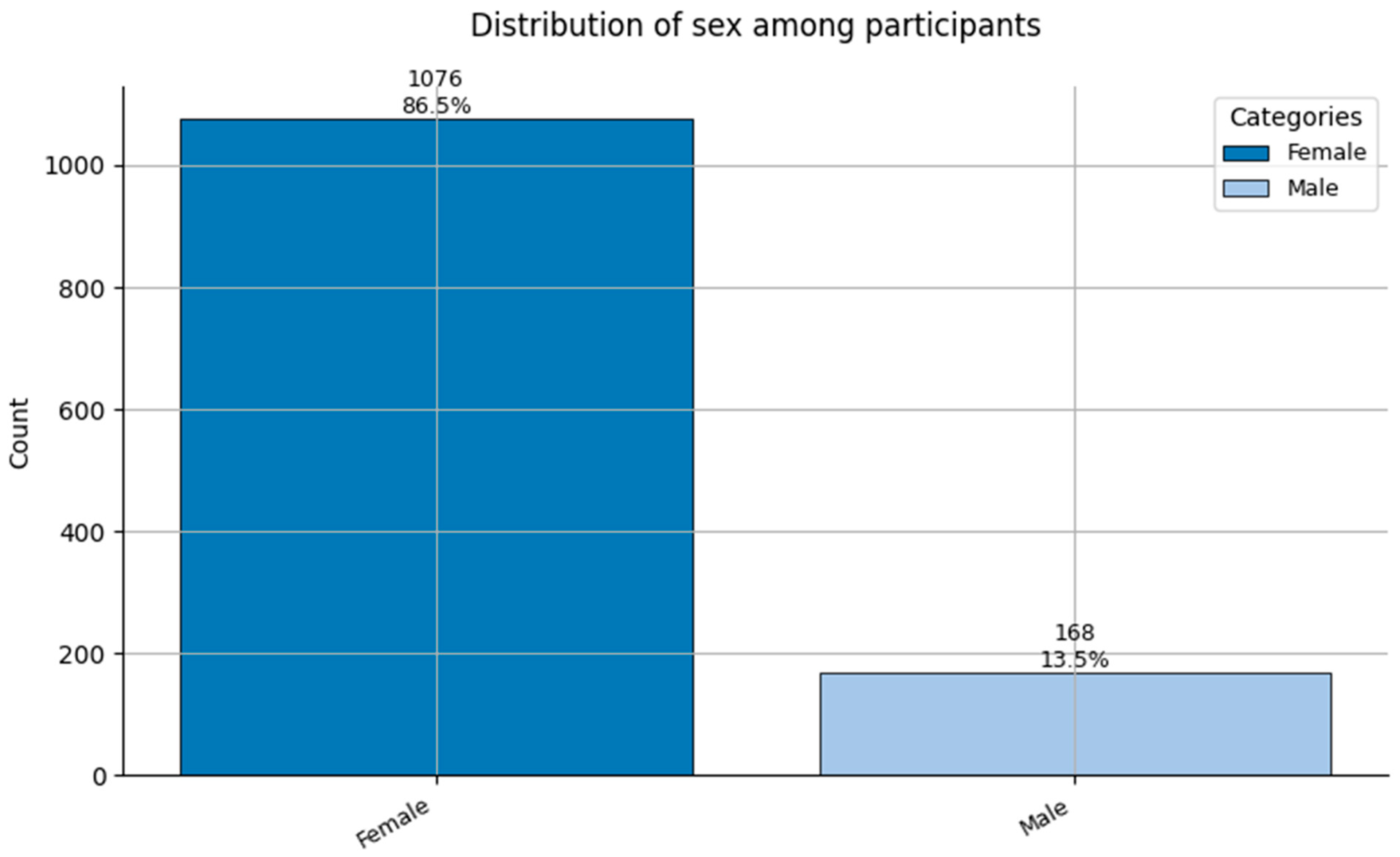
Figure 4.
Distribution of Sex (0 = Female, and 1 = Male) among participants.
Figure 4.
Distribution of Sex (0 = Female, and 1 = Male) among participants.
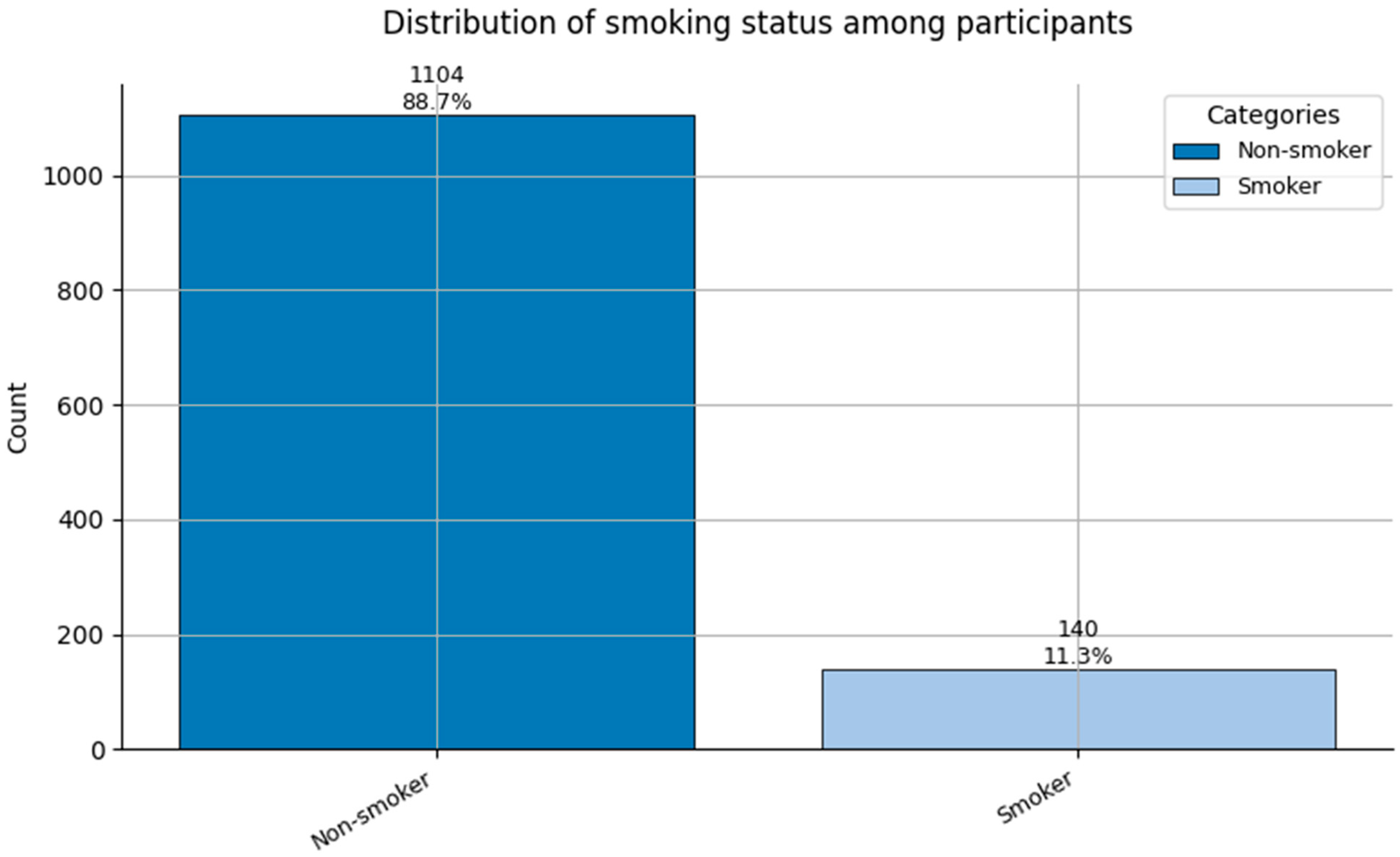
Figure 5.
Distribution of Smoking status (0 = Non-smoker, and 1 = Smoker) among participants.
Figure 5.
Distribution of Smoking status (0 = Non-smoker, and 1 = Smoker) among participants.
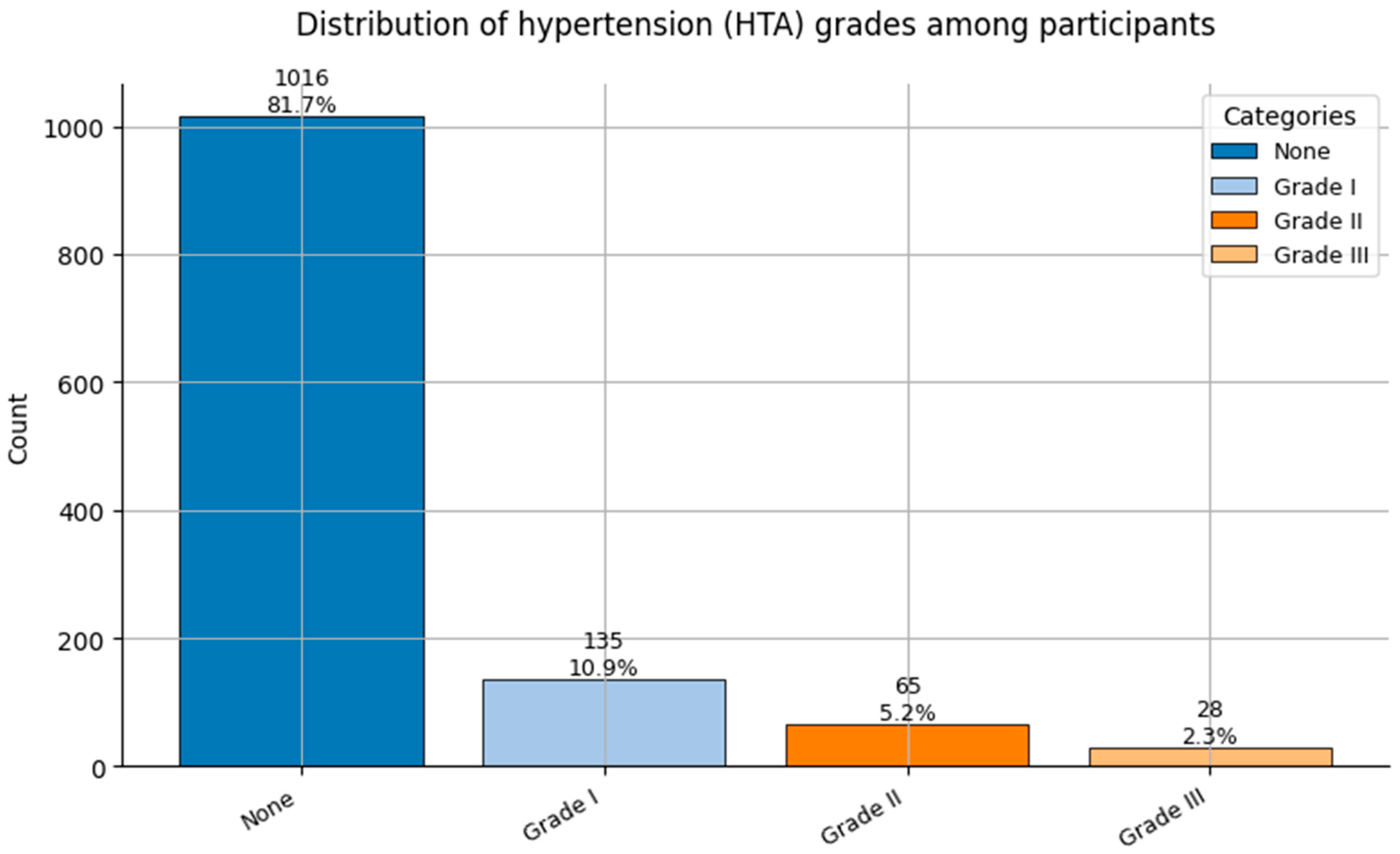
Figure 6.
Distribution of Hypertension grades (HTA; 0 = None, 1 = Grade I, 2 = Grade II, and 3 = Grade III) among participants.
Figure 6.
Distribution of Hypertension grades (HTA; 0 = None, 1 = Grade I, 2 = Grade II, and 3 = Grade III) among participants.
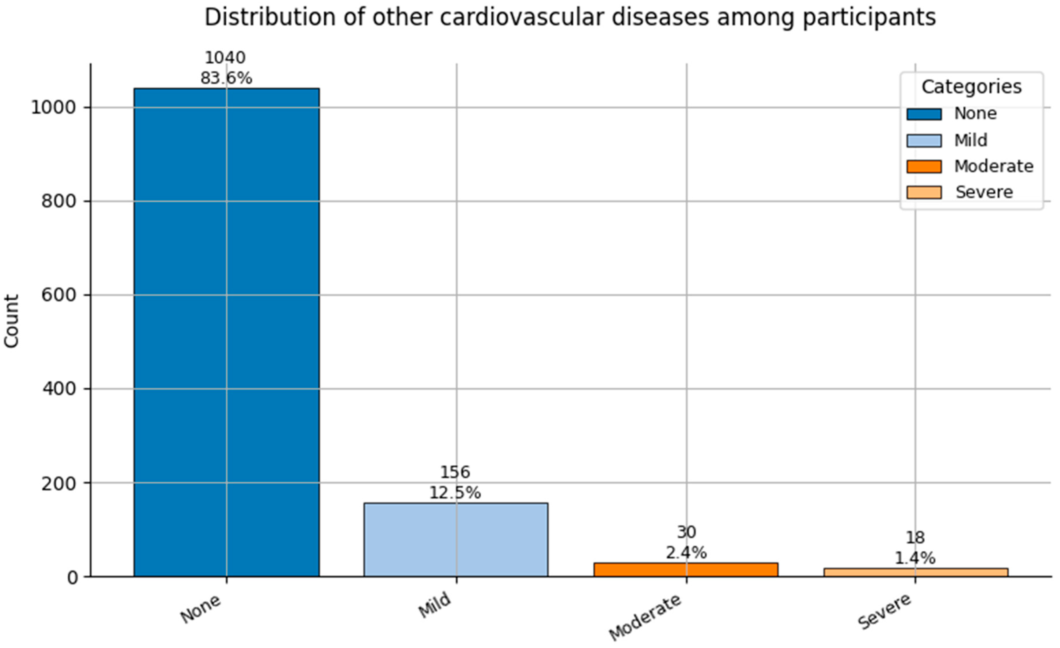
Figure 7.
Distribution of Other Cardiovascular Diseases (0 = None to 3 = Severe) among participants.
Figure 7.
Distribution of Other Cardiovascular Diseases (0 = None to 3 = Severe) among participants.
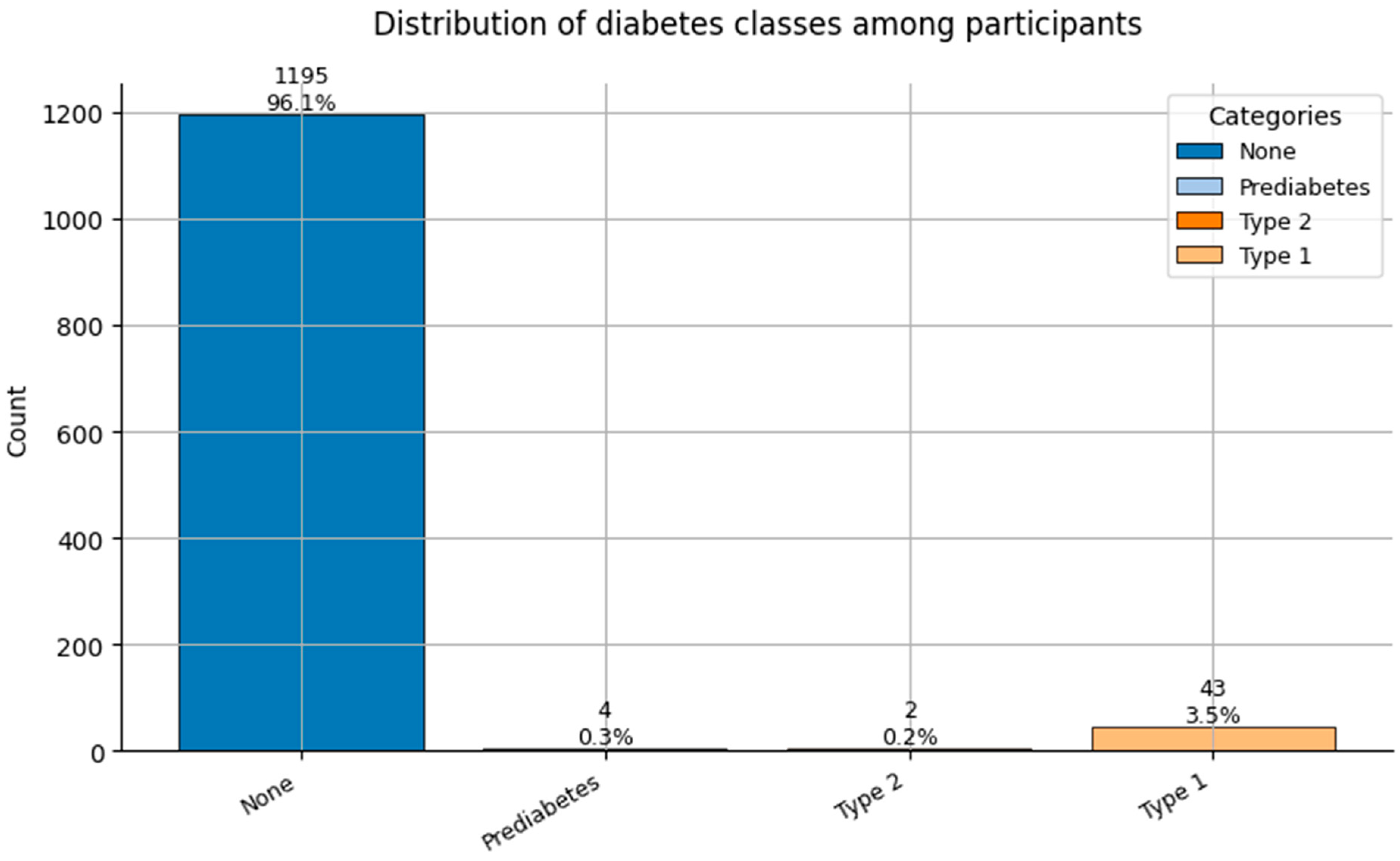
Figure 8.
Distribution of Diabetes classes (0 = None, 1 = Prediabetes, 2 = Type 2, and 3 = Type 1) among participants.
Figure 8.
Distribution of Diabetes classes (0 = None, 1 = Prediabetes, 2 = Type 2, and 3 = Type 1) among participants.
Figure 9.
Distribution of Spinal Conditions (0 = None, 1 = Mild-moderate, and 2 = Surgical/Severe) among participants.
Figure 9.
Distribution of Spinal Conditions (0 = None, 1 = Mild-moderate, and 2 = Surgical/Severe) among participants.
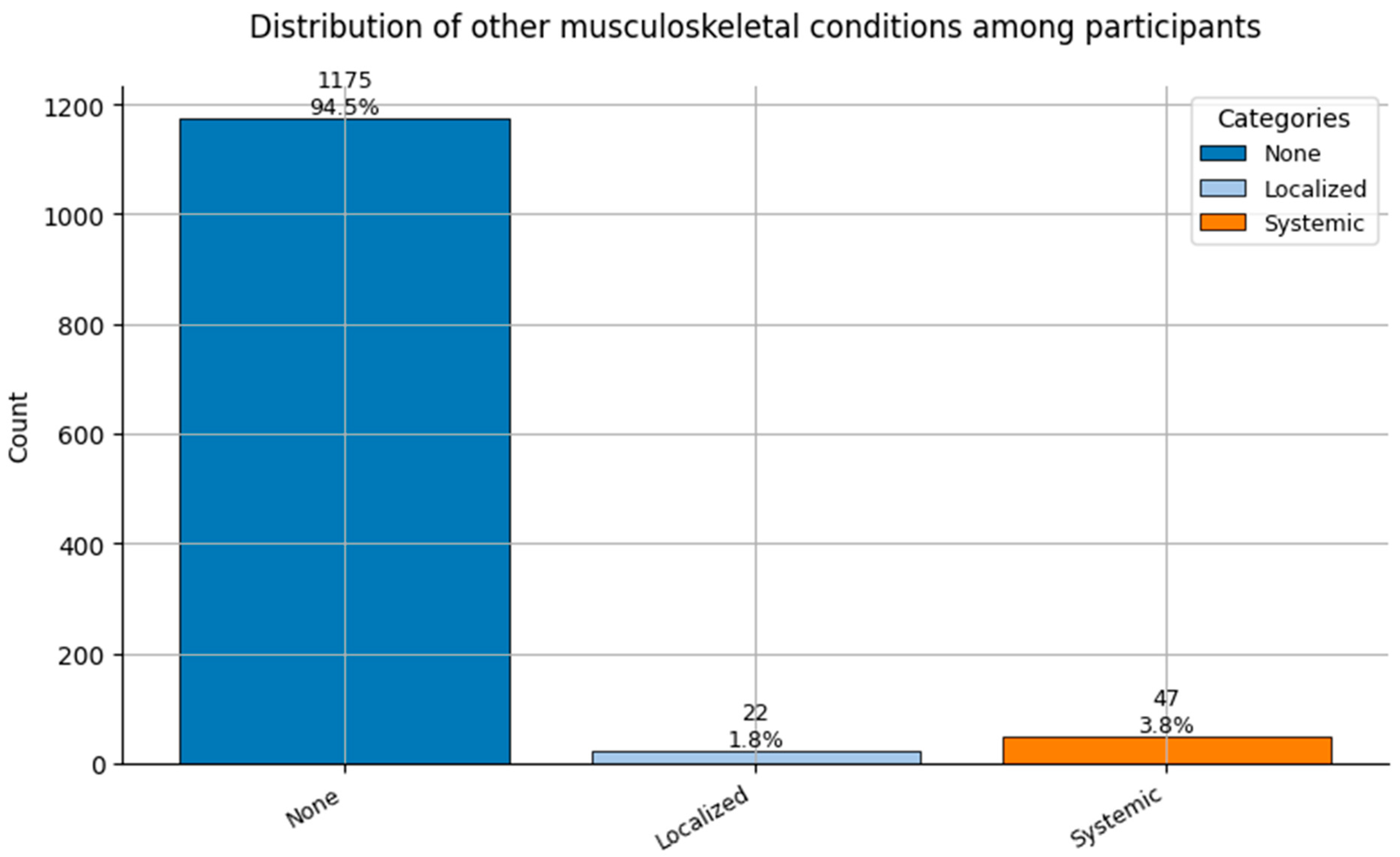
Figure 10.
Distribution of Other Musculoskeletal Conditions (0 = None, 1 = Localized, and 2 = Systemic) among participants.
Figure 10.
Distribution of Other Musculoskeletal Conditions (0 = None, 1 = Localized, and 2 = Systemic) among participants.
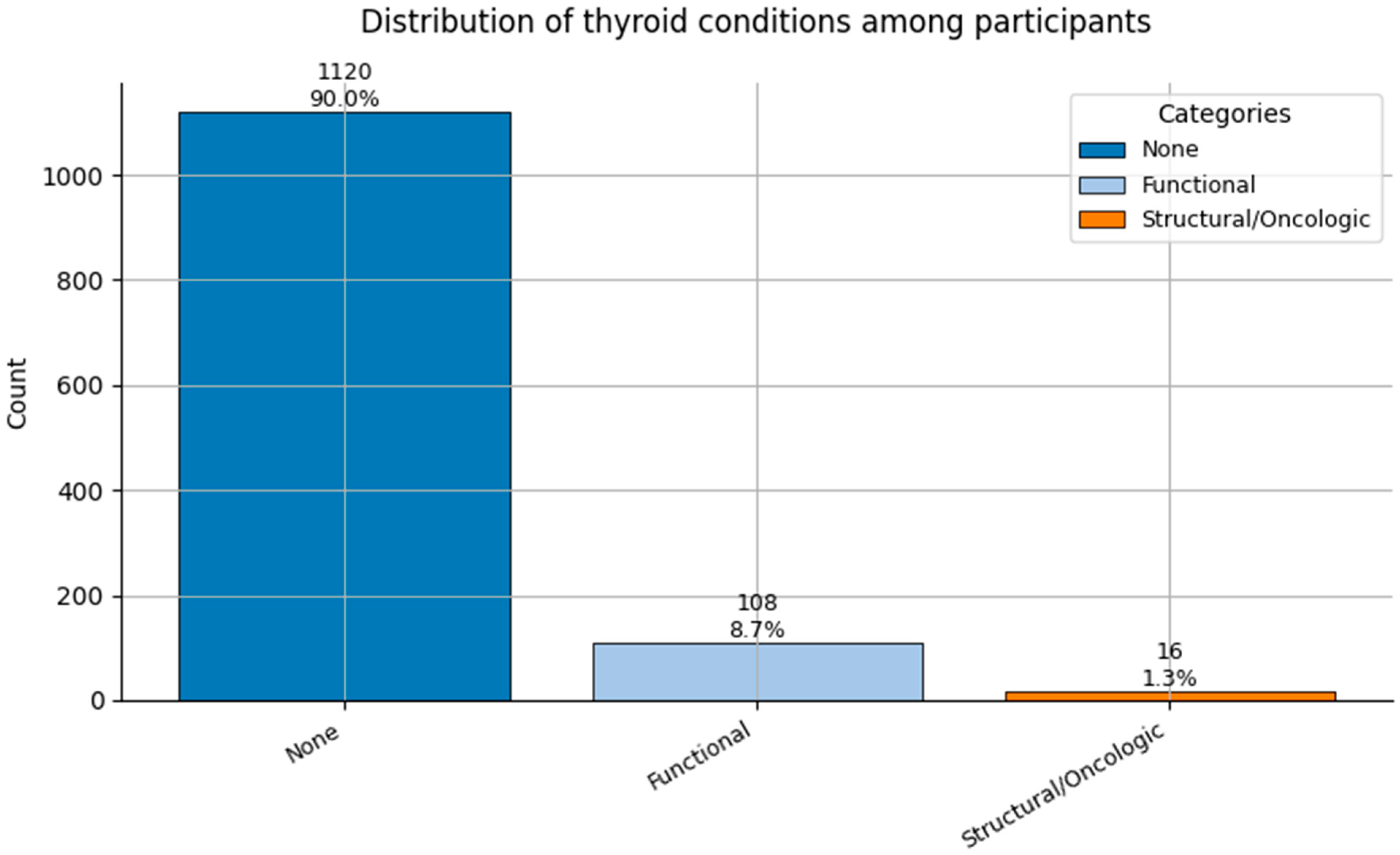
Figure 11.
Distribution of Thyroid Conditions (0 = None, 1 = Functional, and 2 = Structural/Oncologic) among participants.
Figure 11.
Distribution of Thyroid Conditions (0 = None, 1 = Functional, and 2 = Structural/Oncologic) among participants.
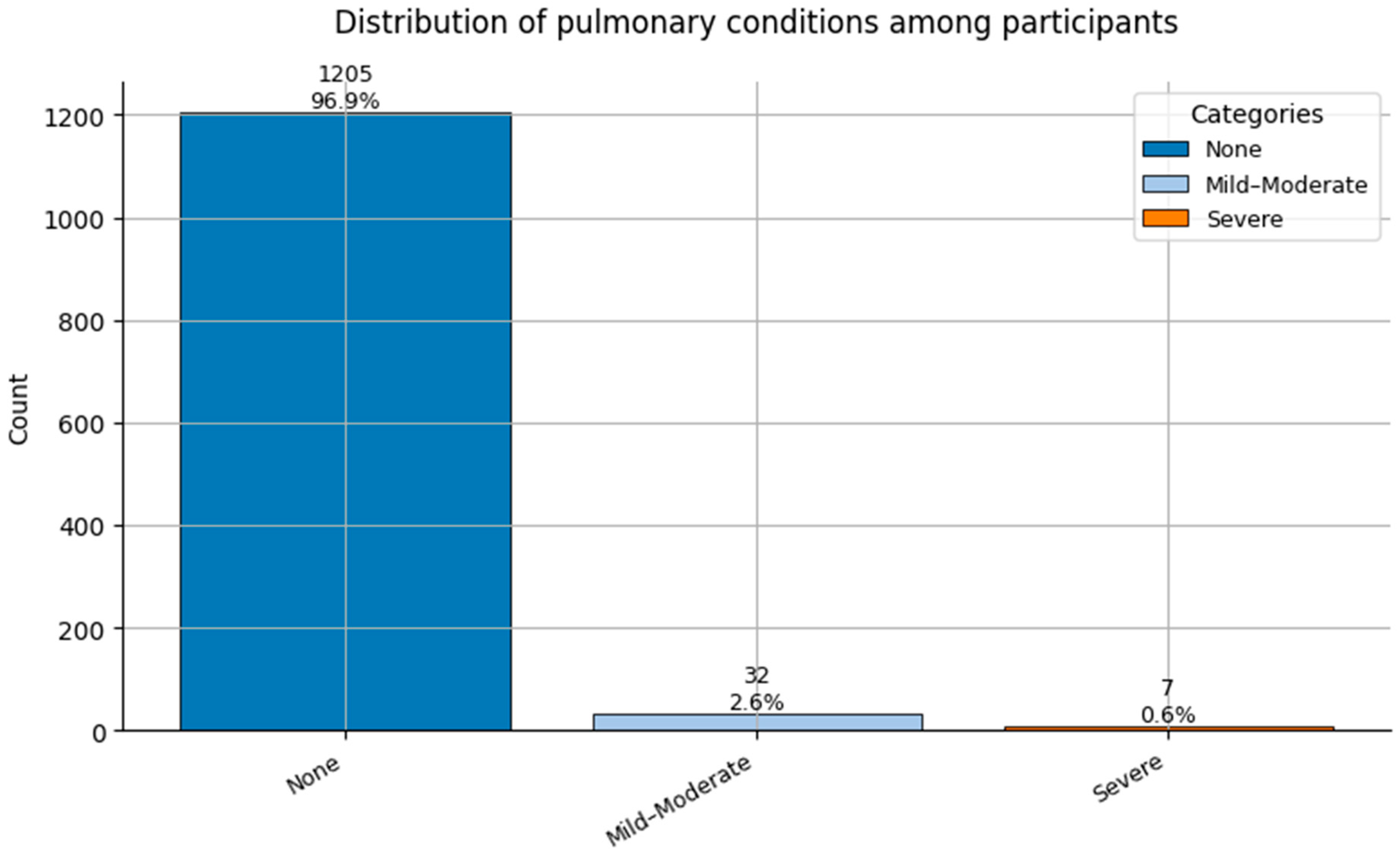
Figure 12.
Distribution of Pulmonary Conditions (0 = None, 1 = Mild-Moderate, and 2 = Severe) among participants.
Figure 12.
Distribution of Pulmonary Conditions (0 = None, 1 = Mild-Moderate, and 2 = Severe) among participants.
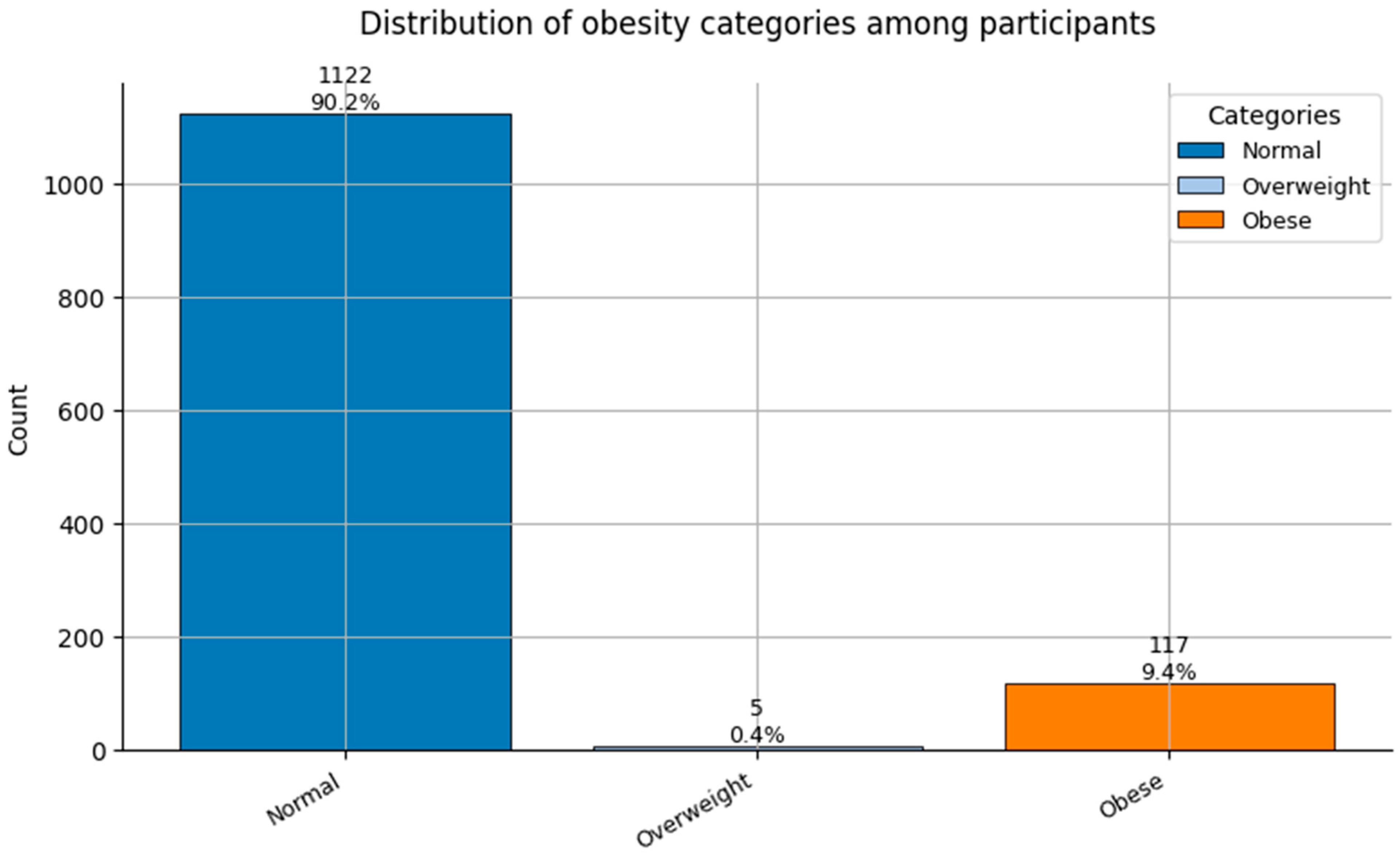
Figure 13.
Distribution of Obesity categories (0 = Normal weight, 1 = Overweight, and 2 = Obese) among participants.
Figure 13.
Distribution of Obesity categories (0 = Normal weight, 1 = Overweight, and 2 = Obese) among participants.
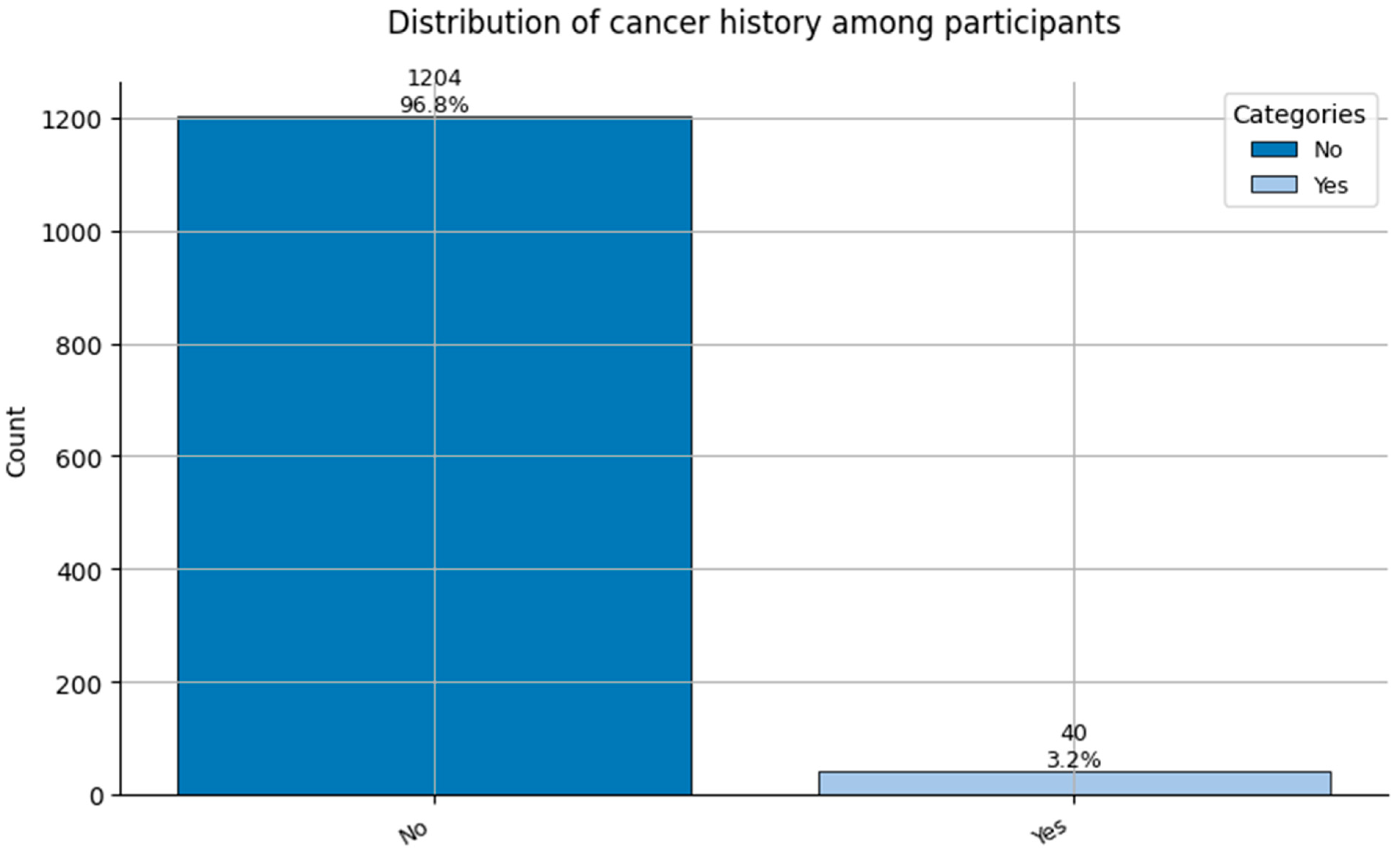
Figure 14.
Distribution of Cancer History (0 = No cancer, and 1 = Cancer history reported) among participants.
Figure 14.
Distribution of Cancer History (0 = No cancer, and 1 = Cancer history reported) among participants.
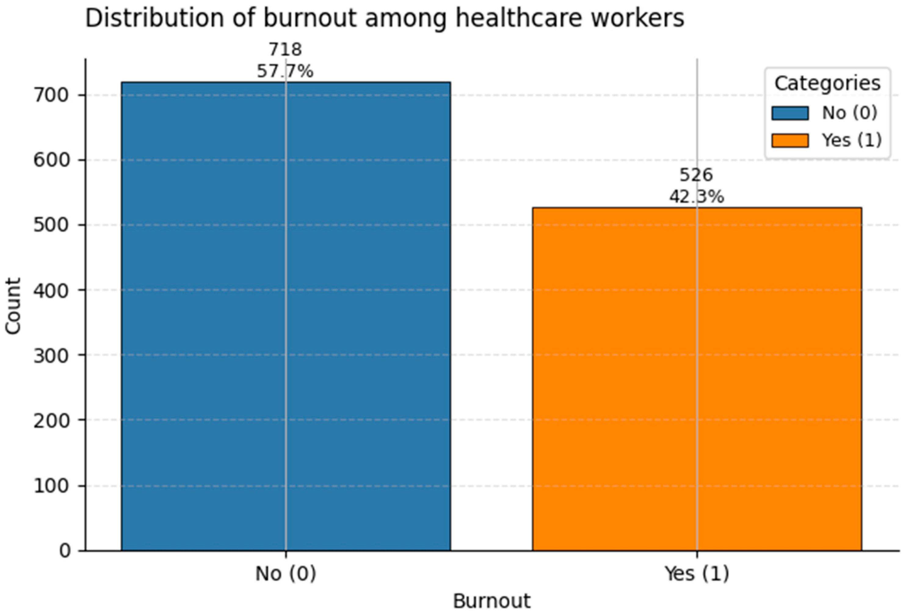
Figure 15.
Distribution of the binary target Burnout among healthcare workers. Class 1 (“Burnout”) accounts for ~42% of the sample.
Figure 15.
Distribution of the binary target Burnout among healthcare workers. Class 1 (“Burnout”) accounts for ~42% of the sample.
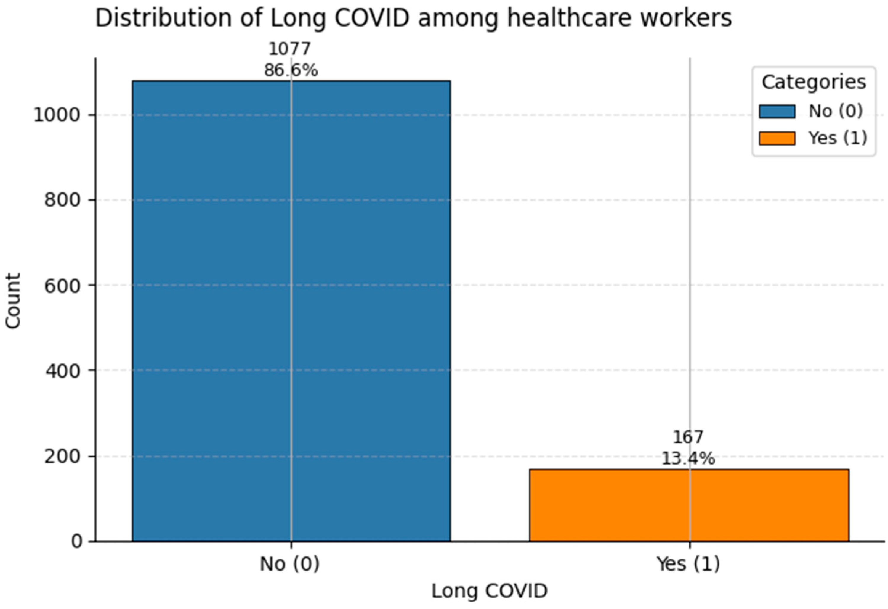
Figure 16.
Frequency of Long COVID reports in the dataset. Class 1 denotes individuals with ongoing post-COVID symptoms (~13%).
Figure 16.
Frequency of Long COVID reports in the dataset. Class 1 denotes individuals with ongoing post-COVID symptoms (~13%).
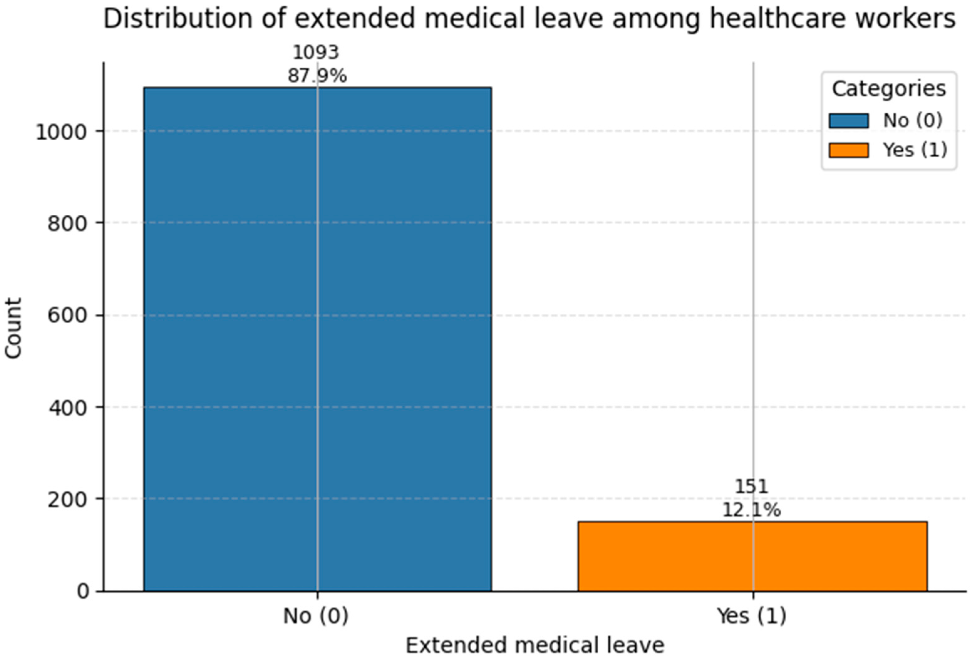
Figure 17.
Count of Extended Medical Leave status in the dataset. Class 1 corresponds to medically documented prolonged leave (~12%).
Figure 17.
Count of Extended Medical Leave status in the dataset. Class 1 corresponds to medically documented prolonged leave (~12%).
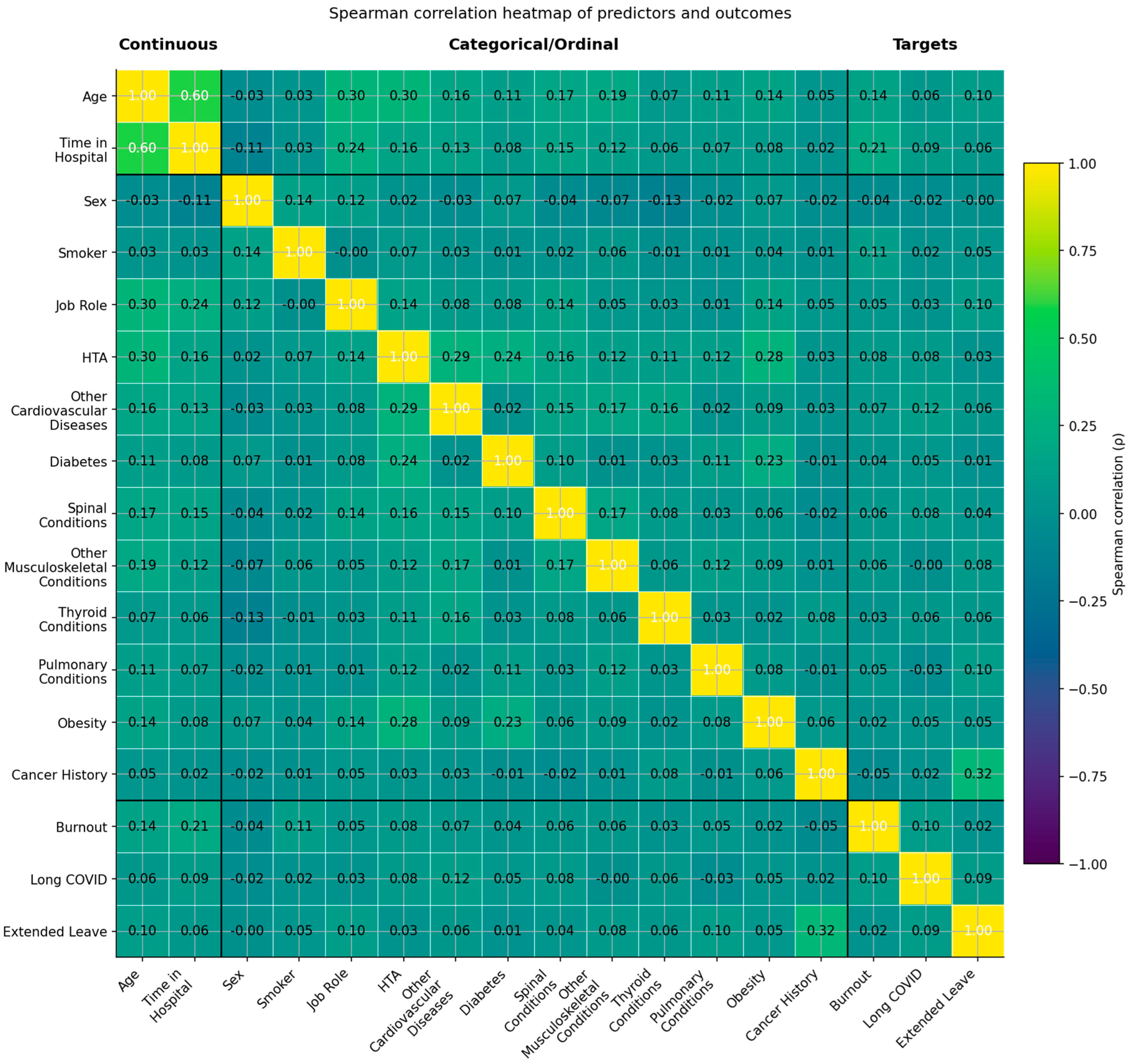
Figure 18.
Spearman correlation heatmap of predictors and outcomes (yellow–green–mauve scale). The heatmap displays rank-based correlations (ρ) among continuous, categorical/ordinal, and target variables. Variables are grouped as Continuous (left), Categorical/Ordinal (middle), and Targets (right). Color intensity follows a sequential palette from yellow (higher positive correlations) through green (moderate) to mauve (negative correlations). Thresholds: |ρ| < 0.10 = negligible; 0.10–0.29 = weak; 0.30–0.49 = moderate; ≥0.50 = strong. Most associations were weak, with moderate clusters observed between Age and Time in Hospital and among cardiometabolic comorbidities.
Figure 19.
t-SNE projection of healthcare worker feature space, colored by Burnout status (0 = No, and 1 = Yes). Intermixed clusters reflect complex, distributed risk.
Figure 19.
t-SNE projection of healthcare worker feature space, colored by Burnout status (0 = No, and 1 = Yes). Intermixed clusters reflect complex, distributed risk.
Figure 20.
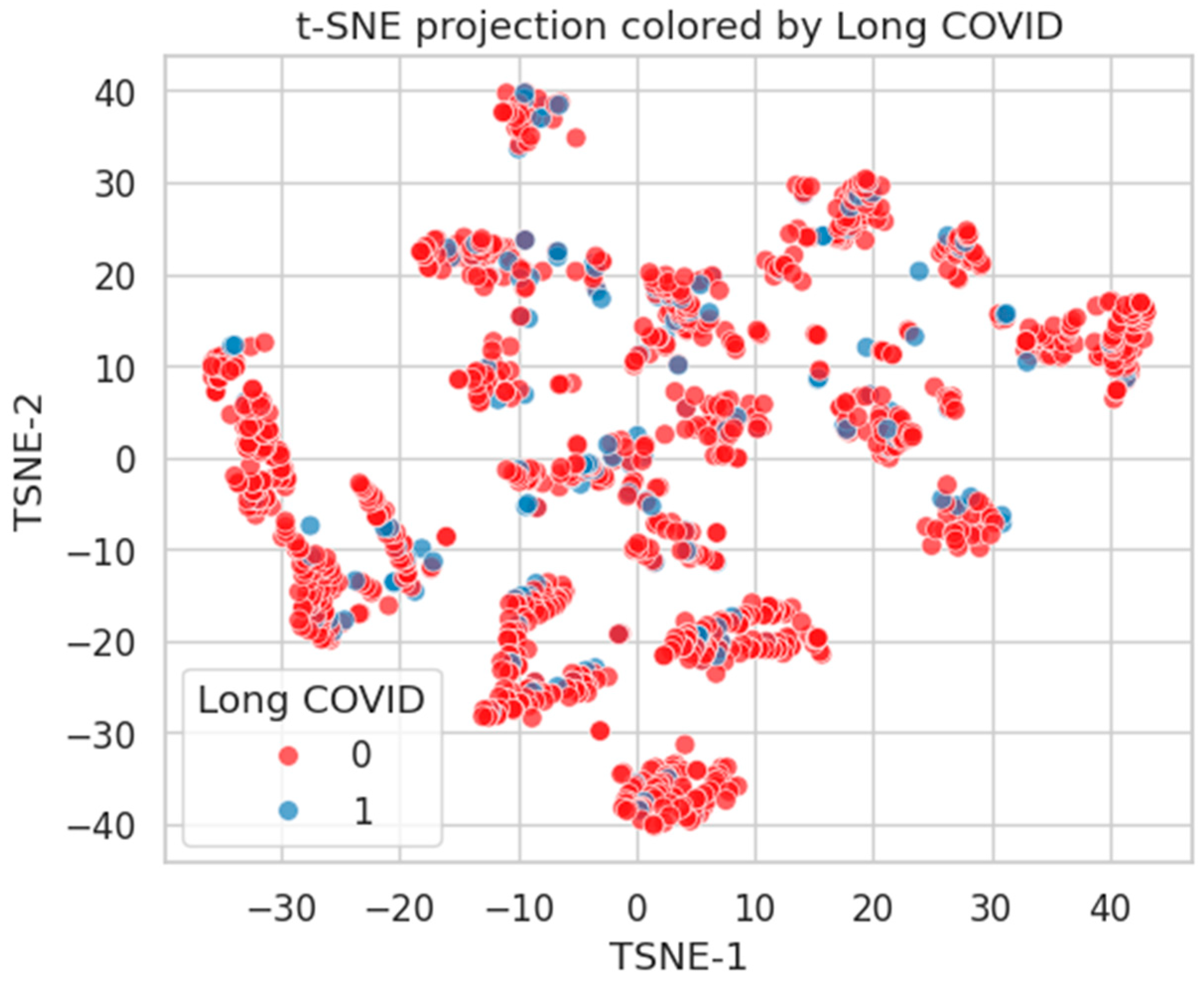
t-SNE projection by Long COVID status. Limited class-wise distinction, indicating diffuse phenotypic representation.
Figure 20.
t-SNE projection by Long COVID status. Limited class-wise distinction, indicating diffuse phenotypic representation.
Figure 21.
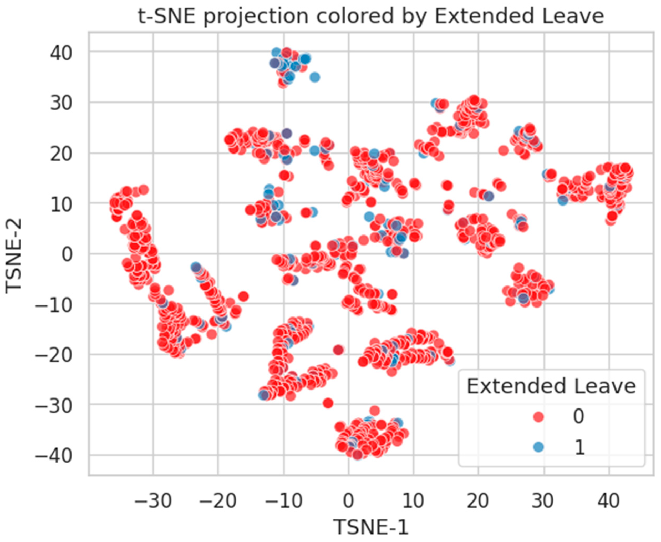
t-SNE embedding by Extended Leave. Moderate clustering of Class 1 suggests stronger alignment with latent health burden.
Figure 21.
t-SNE embedding by Extended Leave. Moderate clustering of Class 1 suggests stronger alignment with latent health burden.
Figure 22.
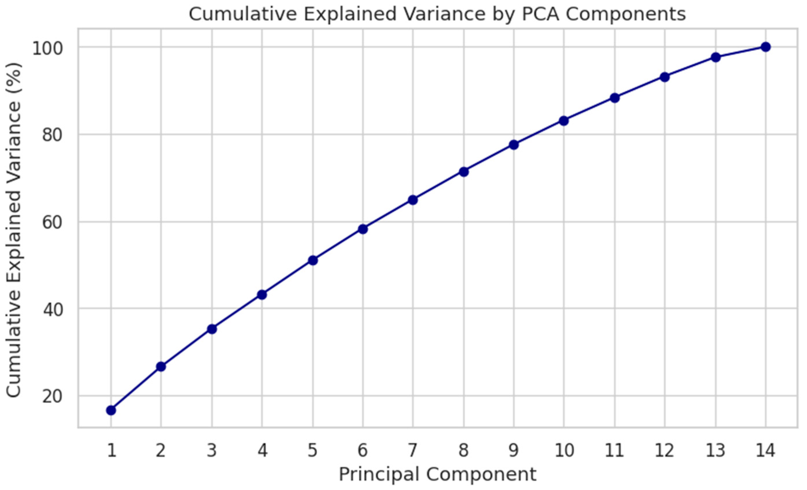
Cumulative explained variance by PCA components. Top 10 PCs account for >75% of total variance.
Figure 22.
Cumulative explained variance by PCA components. Top 10 PCs account for >75% of total variance.
Figure 23.
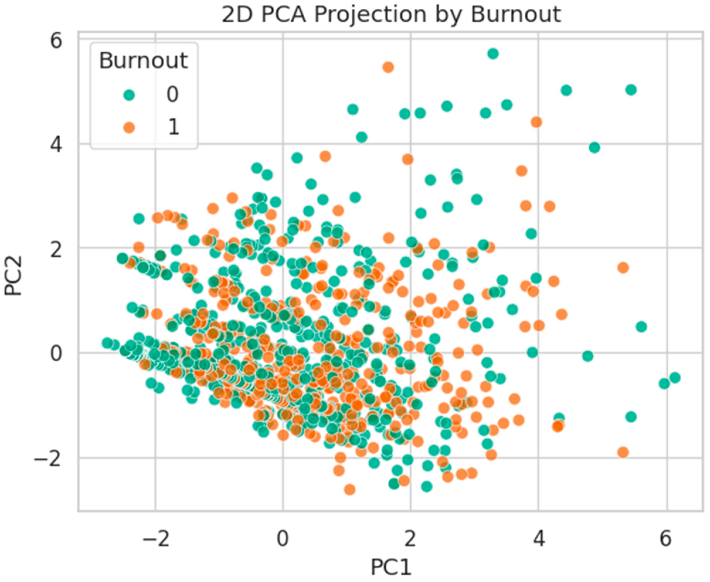
2D PCA projection by Burnout status. Classes are strongly overlapped, with no evident linear boundary.
Figure 23.
2D PCA projection by Burnout status. Classes are strongly overlapped, with no evident linear boundary.
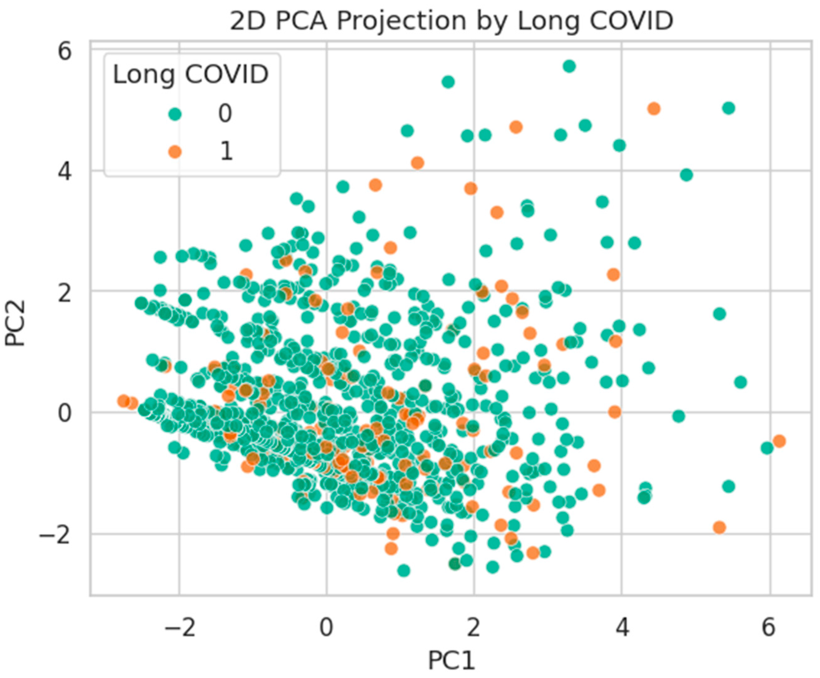
Figure 24.
PCA projection by Long COVID status. Substantial mixing suggests high intra-class heterogeneity.
Figure 24.
PCA projection by Long COVID status. Substantial mixing suggests high intra-class heterogeneity.
Figure 25.
PCA projection by Extended Leave status. Mild class separation along PC1 indicates stronger variance alignment.
Figure 25.
PCA projection by Extended Leave status. Mild class separation along PC1 indicates stronger variance alignment.
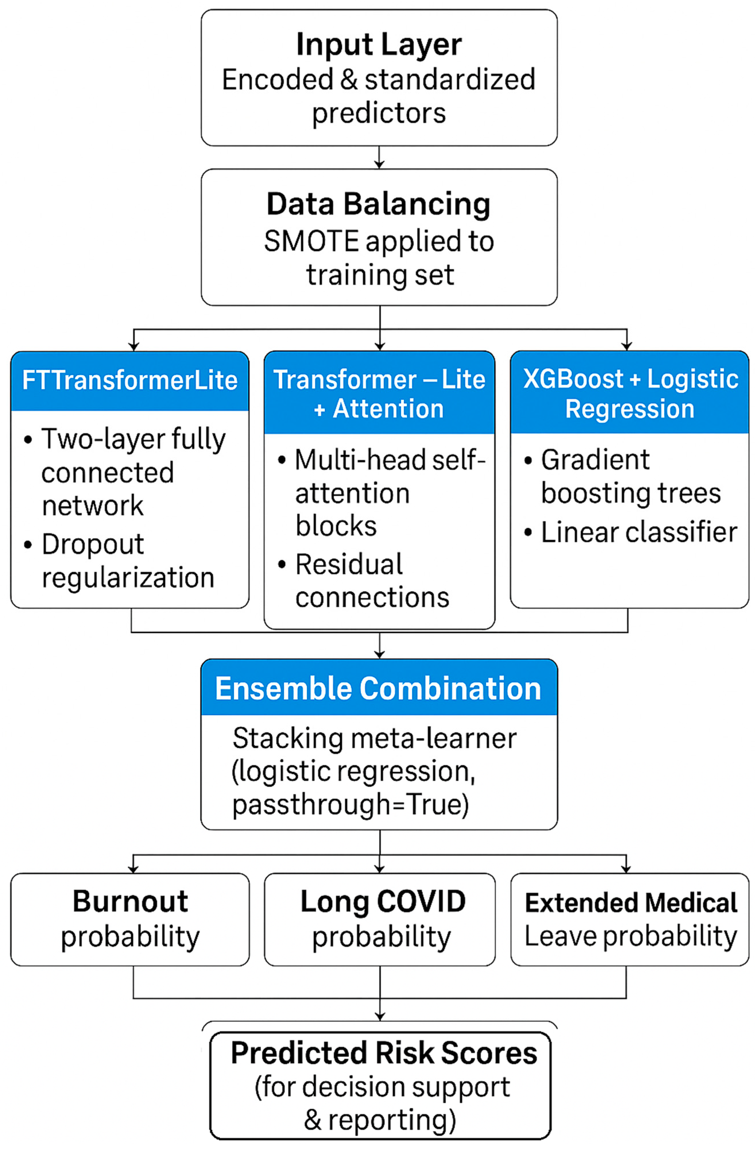
Figure 26.
Machine-learning model pipeline for predicting burnout, Long COVID, and extended medical leave. Encoded and standardized predictors undergo SMOTE balancing before being processed by three modeling pipelines—FTTransformerLite, Transformer-Lite with attention, and XGBoost + logistic regression—followed by an ensemble meta-learner to produce final predicted risk probabilities.
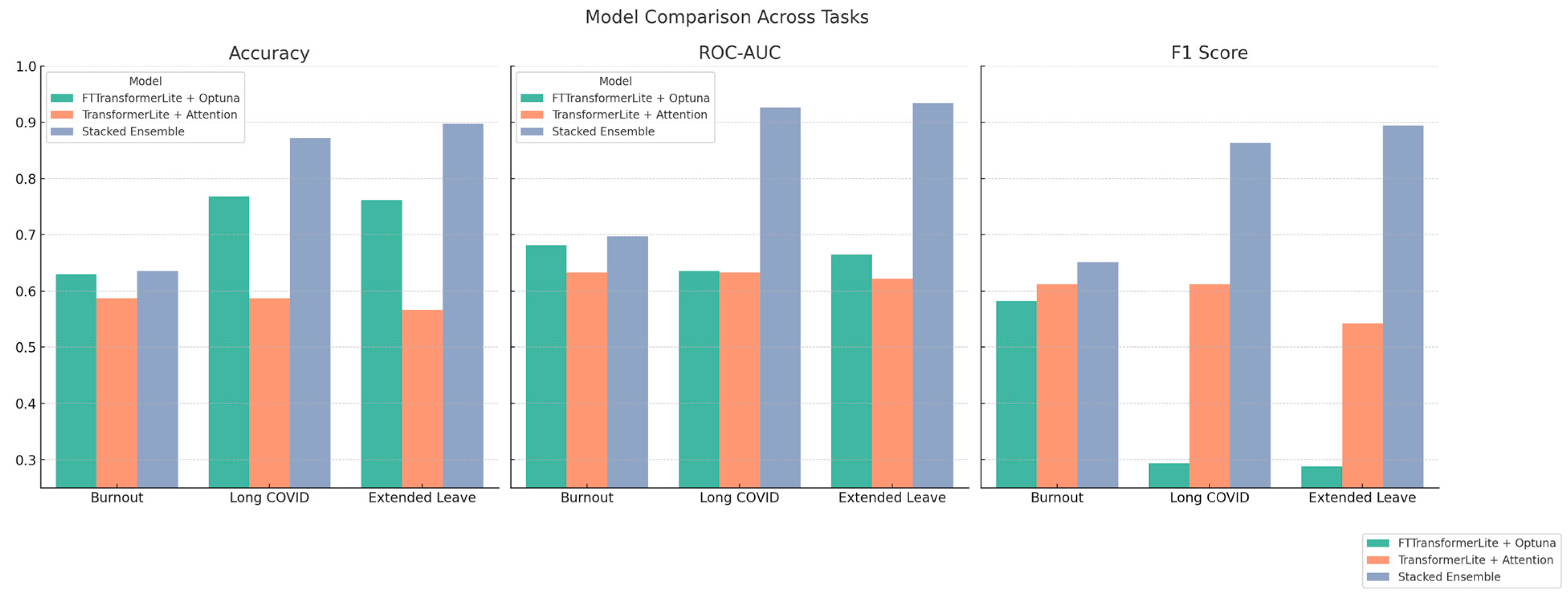
Figure 27.
Comparative performance of predictive models across health outcomes—bar plots showing Accuracy, ROC-AUC, and F1 Score for three models—FTTransformerLite + Optuna (green), TransformerLite + Attention (orange), and Stacked Ensemble (blue)—across prediction tasks for Burnout, Long COVID, and Extended Medical Leave. The Stacked Ensemble consistently demonstrates superior performance, especially in ROC-AUC and F1 Score, indicating improved balance between sensitivity and precision.
Figure 28.
Permutation-based feature importance for predicting Extended Medical Leave. The top 10 most influential features are shown, with chronic health conditions and age among the most predictive indicators.
Figure 28.
Permutation-based feature importance for predicting Extended Medical Leave. The top 10 most influential features are shown, with chronic health conditions and age among the most predictive indicators.
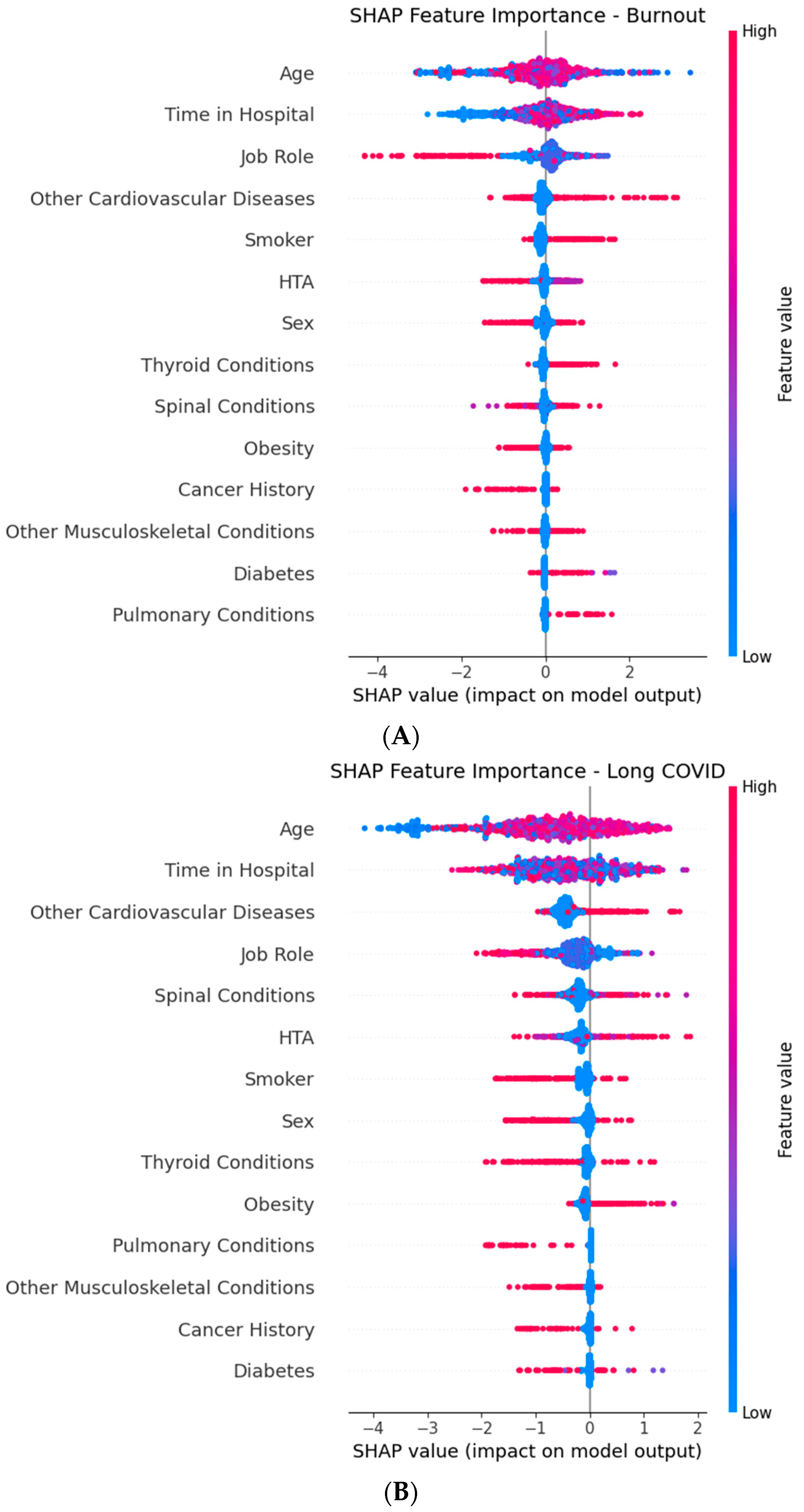
Figure 29.
Global SHAP (SHapley Additive exPlanations) summary plots for the XGBoost component of the Stacked Ensemble, showing the top predictive features for each target outcome: (A) Burnout, (B) Long COVID, and (C) Extended Medical Leave. Each point represents a SHAP value for an individual in the dataset, with color indicating the feature value (red = high, and blue = low). Features are ordered by mean absolute SHAP value (average impact on model output magnitude). Horizontal position shows whether a given feature value increases (positive SHAP value) or decreases (negative SHAP value) the predicted risk. Time in Hospital, Age, Job Role, and chronic comorbidities emerge as key drivers across multiple outcomes.
Figure 30.
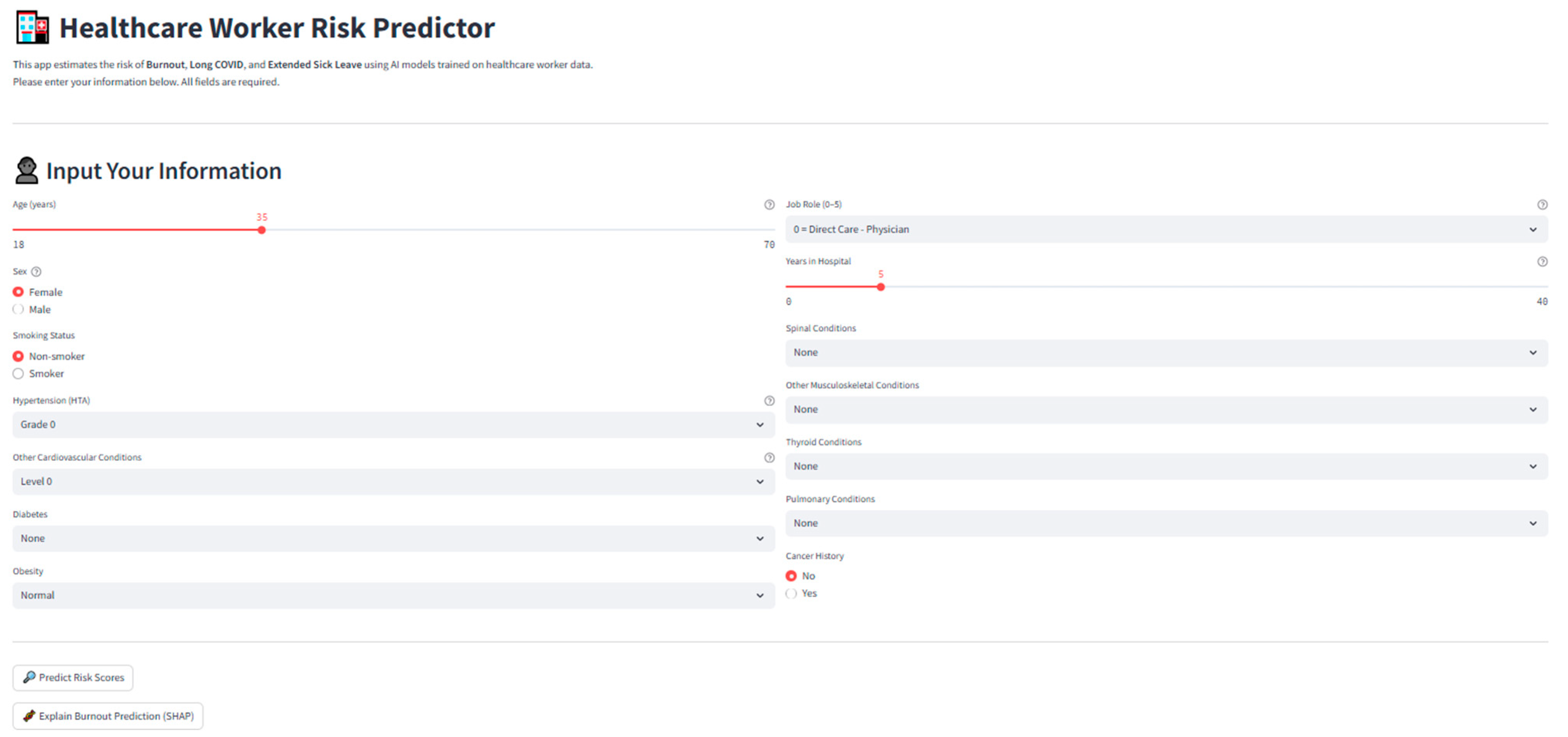
Screenshot of the deployed application interface, showing individual input fields, risk predictions, and SHAP interpretability outputs.
Figure 30.
Screenshot of the deployed application interface, showing individual input fields, risk predictions, and SHAP interpretability outputs.
Figure 31.
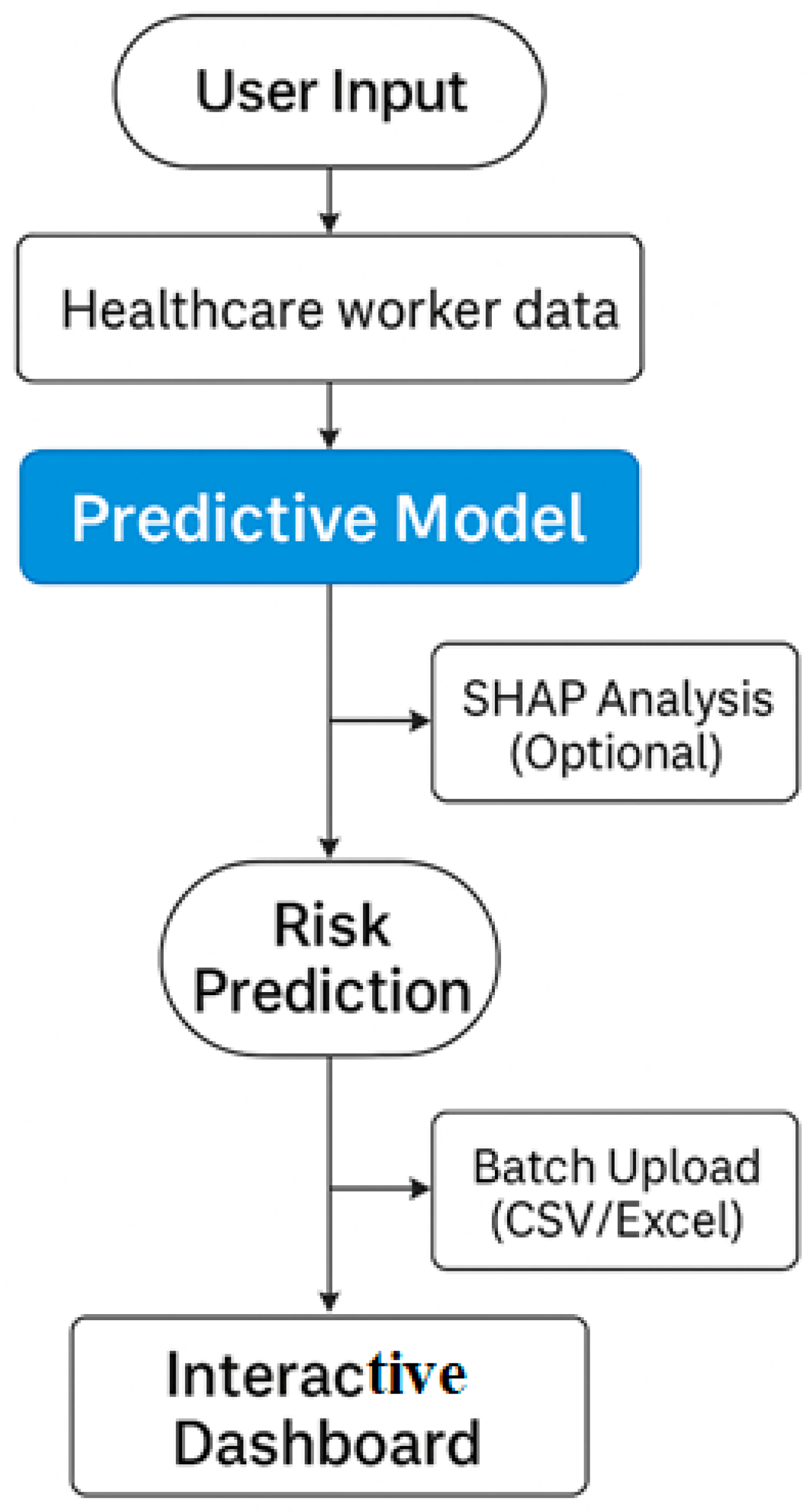
Workflow of the deployed Streamlit application 1.35.0 for healthcare worker risk prediction.
Figure 31.
Workflow of the deployed Streamlit application 1.35.0 for healthcare worker risk prediction.
Table 1.
Clinical and ordinal encoding strategies for comorbidities—summary of medically informed encoding schemes for categorical predictors based on severity and clinical progression.
Table 1.
Clinical and ordinal encoding strategies for comorbidities—summary of medically informed encoding schemes for categorical predictors based on severity and clinical progression.
| Feature | Encoding Strategy |
|---|
| HTA | Ordinal (0–3): Based on ESC/WHO guidelines (Grade 1–3) |
| Other Cardiovascular Diseases | Ordinal (0–3): Mild dyslipidemia to severe heart failure |
| Diabetes | Ordinal (0–3): None, prediabetes, type 1, type 2 |
| Spinal Conditions | Ordinal (0–2): Degeneration → Instability → Surgery |
| Other Musculoskeletal Conditions | Ordinal (0–2): Localized → Systemic/degenerative |
| Thyroid Conditions | Ordinal (0–2): None → Functional → Structural/Oncologic |
| Pulmonary Conditions | Ordinal (0–2): None → Asthma/Apnea → COPD/Fibrosis |
| Obesity | Ordinal (0–2): Normal → Overweight → Obese (Grades I–III) |
| Cancer History | Binary: 0 = No history, 1 = Cancer history |
| Smoker | Binary: 0 = Non-smoker, 1 = Smoker |
Table 2.
Binary encoding of target health outcomes—target labels and their respective binary encoding for classification modeling.
Table 2.
Binary encoding of target health outcomes—target labels and their respective binary encoding for classification modeling.
| Target | Class 0 | Class 1 |
|---|
| Burnout | “No”, 0 | “Yes”, “Burnout” |
| Long COVID | “No”, 0 | “Yes”, “Long COVID symptoms” |
| Extended Sick Leave | “No”, 0 | “Yes”, “Medical Leave” |
Table 3.
Summary of predictor variables: type, encoding scheme, and clinical rationale.
Table 3.
Summary of predictor variables: type, encoding scheme, and clinical rationale.
| Variable | Type | Encoding | Clinical/Occupational Rationale |
|---|
| Job Role | Categorical (Nominal) | Ordinal Grouping (0–5) | Groups reflect exposure risk and work nature (e.g., direct vs. non-clinical care) |
| Sex | Binary | 0 = Female, 1 = Male | Epidemiologically relevant in COVID, burnout, and long leave risk |
| Age | Continuous | Raw (in years) | Age influences comorbidities and recovery outcomes |
| Time in Hospital | Continuous | Raw (years of tenure) | Proxy for occupational exposure duration and cumulative strain |
| Smoker | Binary | 0 = Non-smoker, 1 = Smoker | Risk factor for pulmonary disease, Long COVID, and cardiovascular burden |
| HTA (Hypertension) | Ordinal | 0–3 | Based on WHO/ESC classification: from none to grade III hypertension |
| Other Cardiovascular Diseases | Ordinal | 0–3 | Ranges from mild dyslipidemia to congestive heart failure |
| Diabetes | Ordinal | 0 = None, 1 = Prediabetes, 2 = Type 2, 3 = Type 1 | Progression captures metabolic risk trajectory |
| Spinal Conditions | Ordinal | 0 = None, 1 = Moderate, 2 = Severe/surgical | Reflects biomechanical stress in clinical roles |
| Other Musculoskeletal Conditions | Ordinal | 0 = None, 1 = Localized, 2 = Systemic | Includes repetitive strain or widespread degenerative pathology |
| Thyroid Conditions | Ordinal | 0 = None, 1 = Functional, 2 = Structural/Severe | Captures impact on energy, mood, and metabolic control |
| Pulmonary Conditions | Ordinal | 0 = None, 1 = Mild–Moderate, 2 = Severe | Respiratory impairment linked to work capacity and Long COVID risk |
| Obesity | Ordinal | 0 = Normal, 1 = Overweight, 2 = Obese | Obesity severity is predictive of many health outcomes |
| Cancer History | Binary | 0 = No, 1 = Yes | History of cancer impacts risk of absenteeism, fatigue, and relapse |
Table 4.
Missingness report across predictive features and targets.
Table 4.
Missingness report across predictive features and targets.
| Variable | Missing Values (%) |
|---|
| Job Role | 0.0% |
| Sex | 0.0% |
| Age | 0.0% |
| Time in Hospital | 0.0% |
| Smoker | 0.2% |
| HTA | 0.0% |
| Other Cardiovascular Diseases | 0.0% |
| Diabetes | 0.0% |
| Spinal Conditions | 0.0% |
| Other Musculoskeletal Conditions | 0.0% |
| Thyroid Conditions | 0.0% |
| Pulmonary Conditions | 0.0% |
| Obesity | 0.0% |
| Cancer History | 0.0% |
| Burnout (Target) | 0.2% |
| Long COVID (Target) | 0.4% |
| Extended Sick Leave (Target) | 0.2% |
Table 5.
Hyperparameter search space and optimization ranges used in the Optuna study for tuning the FTTransformerLite model. The study explored categorical, uniform, and log-uniform parameter distributions over 15 trials, with F1 score as the optimization objective.
Table 5.
Hyperparameter search space and optimization ranges used in the Optuna study for tuning the FTTransformerLite model. The study explored categorical, uniform, and log-uniform parameter distributions over 15 trials, with F1 score as the optimization objective.
| Parameter | Range |
|---|
| Hidden dimension | [32, 64, 128] (categorical) |
| Dropout rate | Uniform [0.1, 0.5] |
| Learning rate | Log-uniform [1 × 10⁻⁴, 5 × 10⁻³] |
Table 6.
Classification performance of predictive models for each target outcome.
Table 6.
Classification performance of predictive models for each target outcome.
| Outcome | Model | Accuracy | ROC-AUC | F1 Score |
|---|
| Burnout | FTTransformerLite (Optuna) | 0.5868 | 0.6331 | 0.6124 |
| | Transformer-Lite + Attention | 0.6354 | 0.6974 | 0.6512 |
| | Stacked Ensemble | 0.6354 | 0.6974 | 0.6512 |
| Long COVID | FTTransformerLite (Optuna) | 0.6334 | 0.6738 | 0.6200 |
| | Transformer-Lite + Attention | 0.8724 | 0.9259 | 0.8635 |
| | Stacked Ensemble | 0.8973 | 0.9336 | 0.8941 |
| Ext. Leave | FTTransformerLite (Optuna) | 0.5663 | 0.6223 | 0.5424 |
| | Transformer-Lite + Attention | 0.8724 | 0.9259 | 0.8635 |
| | Stacked Ensemble | 0.8973 | 0.9336 | 0.8941 |
Table 7.
Bootstrapped pairwise comparisons of ROC-AUC performance between the Stacked Ensemble model and two baseline classifiers (Logistic Regression, and Random Forest) across three occupational health outcomes (Burnout, Long COVID, and Extended Leave). Results are reported as the mean difference in AUC (ΔAUC), 95% confidence intervals (CI), and empirical p-values from 10,000 bootstrap resamples. Positive ΔAUC values indicate higher performance for the Stacked Ensemble.
| Outcome | Comparison | Mean ΔAUC | 95% CI | p-Value |
|---|
| Burnout | Ensemble vs. Logistic Regression | 0.0506 | [−0.0030, 0.1065] | 0.0355 |
| Burnout | Ensemble vs. Random Forest | 0.0143 | [−0.0333, 0.0602] | 0.2745 |
| Long COVID | Ensemble vs. Logistic Regression | 0.2955 | [0.2426, 0.3481] | <0.0001 |
| Long COVID | Ensemble vs. Random Forest | −0.0040 | [−0.0198, 0.0121] | 0.3225 |
| Extended Leave | Ensemble vs. Logistic Regression | 0.2083 | [0.1645, 0.2532] | <0.0001 |
| Extended Leave | Ensemble vs. Random Forest | −0.0262 | [−0.0428, −0.0104] | <0.0001 |
Table 8.
Top 10 features for Extended Leave (Random Forest permutation importance).
Table 8.
Top 10 features for Extended Leave (Random Forest permutation importance).
| Rank | Feature | Importance Score |
|---|
| 1 | Cancer History | 0.137 |
| 2 | Pulmonary Conditions | 0.102 |
| 3 | Obesity | 0.098 |
| 4 | Age | 0.081 |
| 5 | Spinal Conditions | 0.079 |
| 6 | Time in Hospital | 0.072 |
| 7 | HTA (Hypertension) | 0.065 |
| 8 | Other Cardiovascular Diseases | 0.057 |
| 9 | Diabetes | 0.049 |
| 10 | Thyroid Conditions | 0.042 |

