
Image Region Prediction from Thermal Videos Based on Image Prediction Generative Adversarial Network


Abstract
1. Introduction
2. Related Works
- -
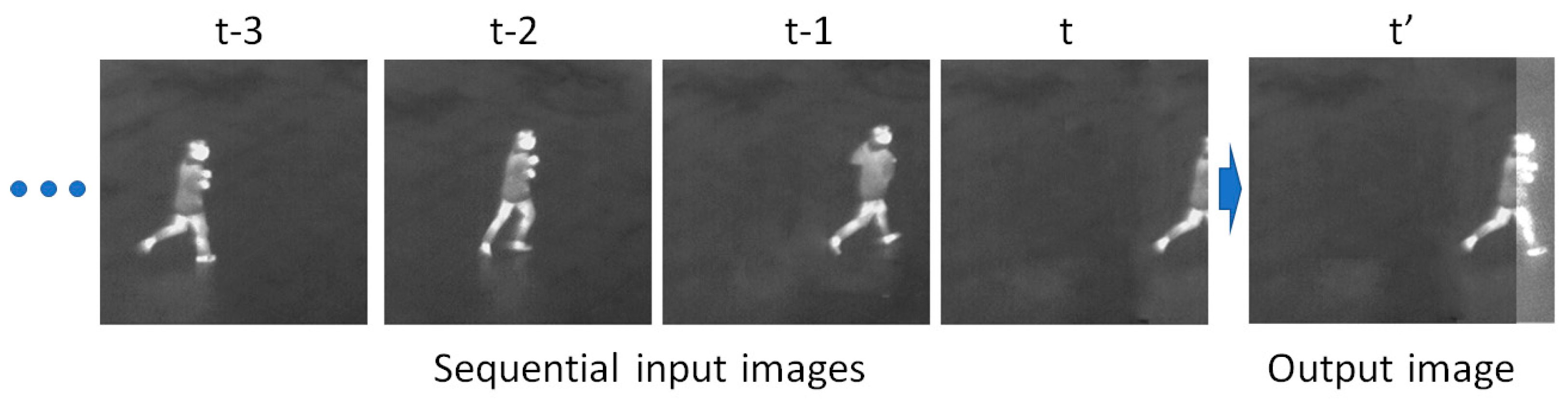
- This study performed image prediction using thermal videos for the first time.
- -
- This study designed an image prediction method that generates an image region outside the FOV for the first time.
- -
- A new IPGAN for performing image prediction is proposed herein.
- -
- The IPGAN model proposed herein is disclosed for a fair performance assessment [28] to other researchers.
3. Materials and Methods
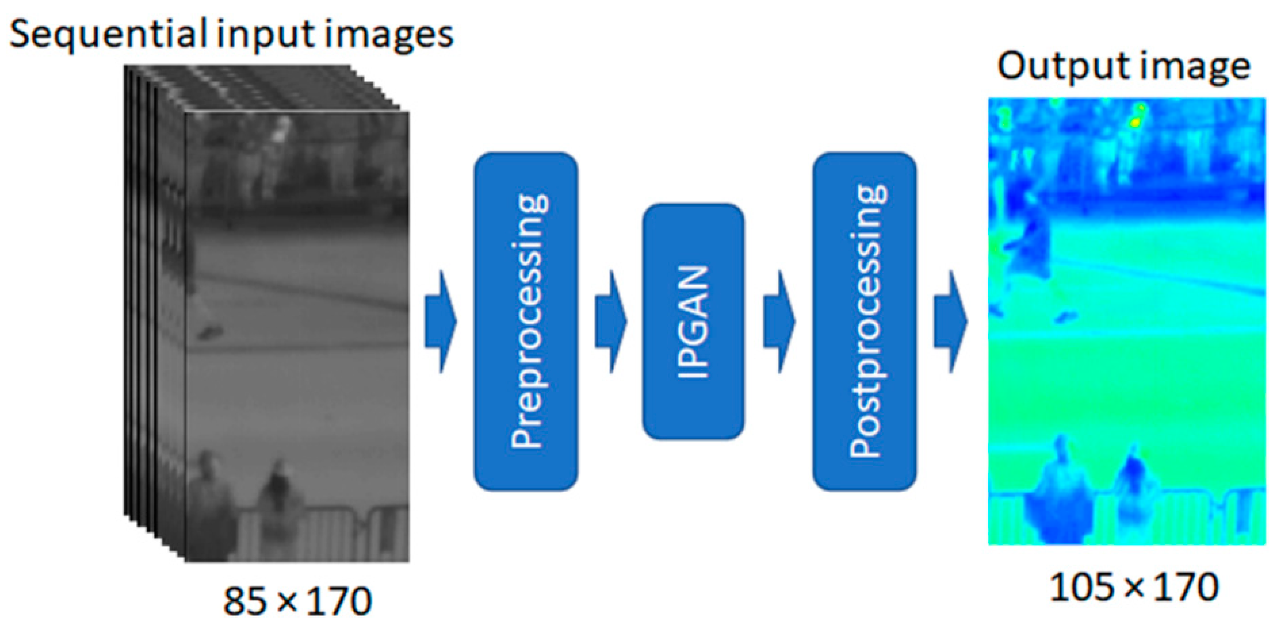
3.1. Overall Procedure of Proposed Method
3.2. Preprocessing
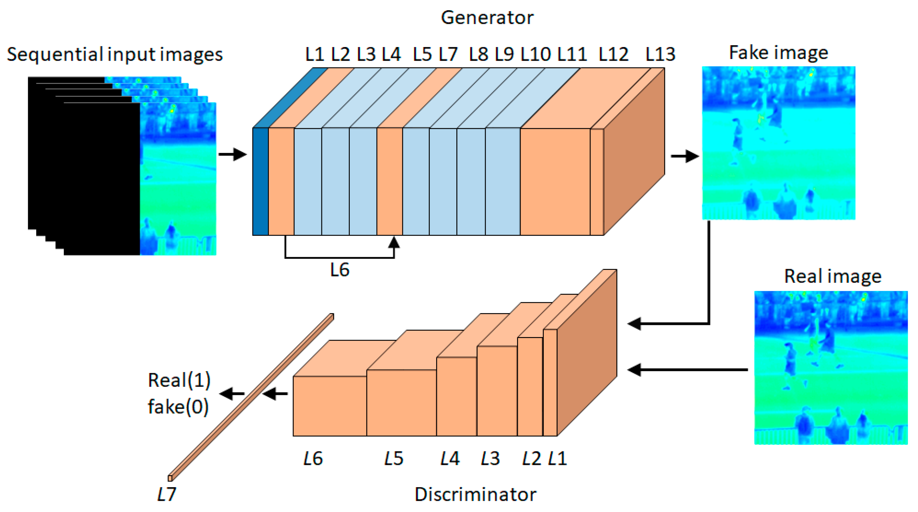
3.3. Proposed IPGAN Model
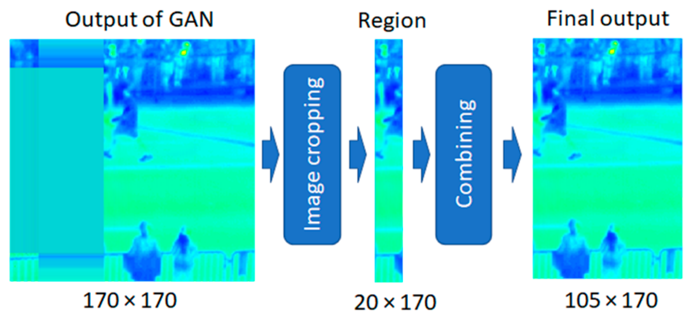
3.4. Postprocessing
3.5. Dataset and Experimental Setup
4. Results
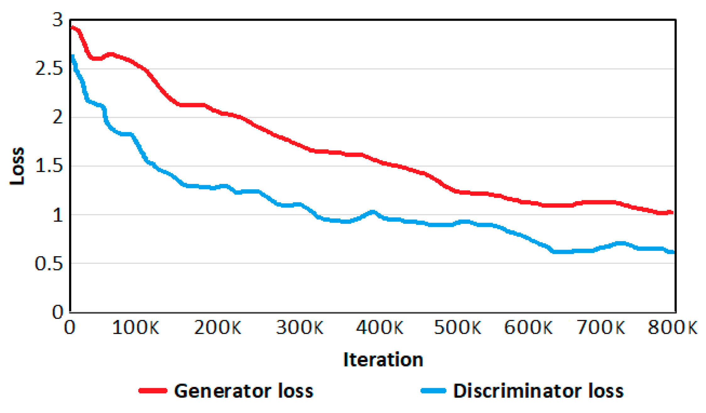
4.1. Training
4.2. Testing (Ablation Study)
4.3. Comparisons of Proposed Method with the State-of-the-Art Methods
4.4. Processing Time
5. Discussion
6. Conclusions
Author Contributions
Funding
Institutional Review Board Statement
Informed Consent Statement
Data Availability Statement
Acknowledgments
Conflicts of Interest
References
- Jeon, E.S.; Kim, J.H.; Hong, H.G.; Batchuluun, G.; Park, K.R. Human detection based on the generation of a background image and fuzzy system by using a thermal camera. Sensors 2016, 16, 453. [Google Scholar] [CrossRef]
- Batchuluun, G.; Kang, J.K.; Nguyen, D.T.; Pham, T.D.; Muhammad, A.; Park, K.R. Deep learning-based thermal image reconstruction and object detection. IEEE Access 2021, 9, 5951–5971. [Google Scholar] [CrossRef]
- Batchuluun, G.; Yoon, H.S.; Nguyen, D.T.; Pham, T.D.; Park, K.R. A study on the elimination of thermal reflections. IEEE Access 2019, 7, 174597–174611. [Google Scholar] [CrossRef]
- Batchuluun, G.; Baek, N.R.; Nguyen, D.T.; Pham, T.D.; Park, K.R. Region-based removal of thermal reflection using pruned fully convolutional network. IEEE Access 2020, 8, 75741–75760. [Google Scholar] [CrossRef]
- Liu, Q.; Li, X.; He, Z.; Fan, N.; Yuan, D.; Wang, H. Learning deep multi-level similarity for thermal infrared object tracking. IEEE Trans. Multimedia 2020. [CrossRef]
- Zulkifley, M.A. Two streams multiple-model object tracker for thermal infrared video. IEEE Access 2019, 7, 32383–32392. [Google Scholar] [CrossRef]
- Zulkifley, M.A.; Trigoni, N. Multiple-model fully convolutional neural networks for single object tracking on thermal infrared video. IEEE Access 2018, 6, 42790–42799. [Google Scholar] [CrossRef]
- Stojanović, M.; Vlahović, N.; Stanković, M.; Stanković, S. Object tracking in thermal imaging using kernelized correlation filters. In Proceedings of the 17th International Symposium INFOTEH-JAHORINA (INFOTEH), East Sarajevo, Bosnia and Herzegovina, 21–23 March 2018. [Google Scholar]
- Asha, C.S.; Narasimhadhan, A.V. Experimental evaluation of feature channels for object tracking in RGB and thermal imagery using correlation filter. In Proceedings of the Twenty-third National Conference on Communications (NCC), Chennai, India, 2–4 March 2017. [Google Scholar]
- Batchuluun, G.; Kim, Y.G.; Kim, J.H.; Hong, H.G.; Park, K.R. Robust behavior recognition in intelligent surveillance environments. Sensors 2016, 16, 1010. [Google Scholar] [CrossRef]
- Batchuluun, G.; Kim, J.H.; Hong, H.G.; Kang, J.K.; Park, K.R. Fuzzy system based human behavior recognition by combining behavior prediction and recognition. Expert Syst. Appl. 2017, 81, 108–133. [Google Scholar] [CrossRef]
- Batchuluun, G.; Nguyen, D.T.; Pham, T.D.; Park, C.; Park, K.R. Action recognition from thermal videos. IEEE Access 2019, 7, 103893–103917. [Google Scholar] [CrossRef]
- Mun, J.-H.; Jeon, M.; Lee, B.-G. Unsupervised learning for depth, ego-motion, and optical flow estimation using coupled consistency conditions. Sensors 2019, 19, 2459. [Google Scholar] [CrossRef]
- Wu, Z.; Fuller, N.; Theriault, D.; Betke, M. A thermal infrared video benchmark for visual analysis. In Proceedings of the IEEE Conference on Computer Vision and Pattern Recognition Workshops, Columbus, OH, USA, 23–28 June 2014. [Google Scholar]
- Haziq, R.; Basura, F. A log-likelihood regularized KL divergence for video prediction with a 3D convolutional variational recurrent network. In Proceedings of the IEEE/CVF Winter Conference on Applications of Computer Vision Workshops, Waikola, HI, USA, 5–9 January 2021. [Google Scholar]
- Guen, V.L.; Thome, N. Disentangling physical dynamics from unknown factors for unsupervised video prediction. In Proceedings of the IEEE Conference on Computer Vision and Pattern Recognition, Seattle, WA, USA, 13–19 June 2020. [Google Scholar]
- Finn, C.; Goodfellow, I.; Levine, S. Unsupervised learning for physical interaction through video prediction. In Proceedings of the Advances in Neural Information Processing Systems 29, Barcelona, Spain, 5–10 December 2016. [Google Scholar]
- Xu, J.; Xu, H.; Ni, B.; Yang, X.; Darrell, T. Video prediction via example guidance. In Proceedings of the 37th International Conference on Machine Learning, Online, 13–18 July 2020. [Google Scholar]
- Babaeizadeh, M.; Finn, C.; Erhan, D.; Campbell, R.H.; Levine, S. Stochastic variational video prediction. In Proceedings of the 6th International Conference on Learning Representations, Vancouver, BC, Canada, 30 April–3 May 2018. [Google Scholar]
- Liu, H.; Jiang, B.; Xiao, Y.; Yang, C. Coherent semantic attention for image inpainting. In Proceedings of the IEEE/CVF International Conference on Computer Vision Workshop, Seoul, Korea, 27 October–2 November 2019. [Google Scholar]
- Yu, J.; Lin, Z.; Yang, J.; Shen, X.; Lu, X.; Huang, T. Free-form image inpainting with gated convolution. In Proceedings of the IEEE/CVF International Conference on Computer Vision Workshop, Seoul, Korea, 27 October–2 November 2019. [Google Scholar]
- Shin, Y.-G.; Sagong, M.-C.; Yeo, Y.-J.; Kim, S.-W.; Ko, S.-J. PEPSI++: Fast and lightweight network for image inpainting. IEEE Trans. Neural Netw. Learn. Syst. 2021, 32, 252–265. [Google Scholar] [CrossRef]
- Pathak, D.; Krähenbühl, P.; Donahue, J.; Darrell, T.; Efros, A.A. Context encoders: Feature learning by inpainting. In Proceedings of the IEEE Conference on Computer Vision and Pattern Recognition, Las Vegas, NV, USA, 27–30 June 2016. [Google Scholar]
- Nazeri, K.; Ng, E.; Joseph, T.; Qureshi, F.; Ebrahimi, M. EdgeConnect: Structure guided image inpainting using edge prediction. In Proceedings of the IEEE/CVF International Conference on Computer Vision Workshop, Seoul, Korea, 27 October–2 November 2019. [Google Scholar]
- Oprea, S.; Martinez-Gonzalez, P.; Garcia-Garcia, A.; Castro-Vargas, J.A.; Orts-Escolano, S.; Garcia-Rodriguez, J.; Argyros, A. A review on deep learning techniques for video prediction. IEEE Trans. Pattern Anal. Mach. Intell. 2020. [CrossRef]
- Rasouli, A. Deep learning for vision-based prediction: A survey. arXiv 2020, arXiv:2007.00095v2. [Google Scholar]
- Elharrouss, O.; Almaadeed, N.; Al-Maadeed, S.; Akbari, Y. Image inpainting: A review. Neural Process. Lett. 2020, 51, 2007–2028. [Google Scholar] [CrossRef]
- Image Prediction Generative Adversarial Network (IPGAN). Available online: http://dm.dgu.edu/link.html (accessed on 25 March 2021).
- MathWorks. Available online: https://www.mathworks.com/help/matlab/ref/jet.html (accessed on 25 March 2021).
- Batchuluun, G.; Lee, Y.W.; Nguyen, D.T.; Pham, T.D.; Park, K.R. Thermal image reconstruction using deep learning. IEEE Access 2020, 8, 126839–126858. [Google Scholar] [CrossRef]
- Batchuluun, G.; Kang, J.K.; Nguyen, D.T.; Pham, T.D.; Arsalan, M.; Park, K.R. Action recognition from thermal videos using joint and skeleton information. IEEE Access 2021, 9, 11716–11733. [Google Scholar] [CrossRef]
- Funt, B.; Zhu, L. Does colour really matter? Evaluation via object classification. In Proceedings of the 26th Color and Imaging Conference Final Program and Proceedings, Vancouver, BC, Canada, 12–16 November 2018. [Google Scholar]
- NVIDIA Corporation. Available online: https://www.nvidia.com/en-us/geforce/products/10series/titan-x-pascal/ (accessed on 25 March 2021).
- OpenCV. Available online: http://opencv.org/ (accessed on 25 March 2021).
- Keras. Available online: https://keras.io/ (accessed on 25 March 2021).
- Kingma, D.P.; Ba, J.L. Adam: A method for stochastic optimization. arXiv 2014, arXiv:1412.6980. [Google Scholar]
- Mean Squared Error. Available online: https://en.wikipedia.org/wiki/Mean_squared_error (accessed on 29 April 2021).
- Peak Signal-to-Noise Ratio. Available online: https://en.wikipedia.org/wiki/Peak_signal-to-noise_ratio (accessed on 29 April 2021).
- Structural Similarity. Available online: https://en.wikipedia.org/wiki/Structural_similarity (accessed on 29 April 2021).
- Huynh-Thu, Q.; Ghanbari, M. The Accuracy of PSNR in predicting video quality for different video scenes and frame rates. Telecommun. Syst. 2012, 49, 35–48. [Google Scholar] [CrossRef]
- Huynh-Thu, Q.; Ghanbari, M. Scope of validity of PSNR in image/video quality assessment. Electron. Lett. 2008, 44, 800–801. [Google Scholar] [CrossRef]
- He, K.; Gkioxari, G.; Dollár, P.; Girshick, R. Mask R-CNN. In Proceedings of the IEEE International Conference on Computer Vision, Venice, Italy, 22–29 October 2017. [Google Scholar]
- Powers, D.M.W. Evaluation: From precision, recall and f-measure to ROC, informedness, markedness & correlation. Mach. Learn. Technol. 2011, 2, 37–63. [Google Scholar]
- Derczynski, L. Complementarity, f-score, and NLP evaluation. In Proceedings of the International Conference on Language Resources and Evaluation, Portorož, Slovenia, 23–28 May 2016. [Google Scholar]


| Category | Methods | Advantages | Disadvantages | |
|---|---|---|---|---|
| Using visible-light images | Future image prediction | Encoder–decoder model [15,18], PhyDNet [16], CNN + LSTM [17], SV2P [19], and review and survey [25,26] | High performance of future image prediction based on a current frame and previous frames | Do not consider the image prediction out of FOV Do not use thermal image of low resolution and low image quality |
| Image inpainting | CSA layer [20], gated convolution + SN-PatchGAN [21], PEPSI [22], context encoder [23], edge prediction and image completion [24], and review [27] | High performance of image inpainting based on a current frame | ||
| Using thermal images | Image region prediction out of FOV | Three-channel thermal image and IPGAN (proposed method) | Consider the image prediction out of FOV Use thermal image of low resolution and low image quality | The predicted image out of FOV has a size limit |
| Layer Number | Layer Type | Number of Filters | Number of Parameters | Layer Connection (Connected to) |
|---|---|---|---|---|
| 0 | input_layers_1–20 | 0 | 0 | input_1–20 |
| 1 | concat | 0 | 0 | input_layers_1–20 |
| 2 | conv_block_1 | 128/64 | 143,232 | concat |
| 3 | res_block_1 | 64 | 73,920 | conv_block_1 |
| 4 | res_block_2 | 64 | 73,920 | res_block_1 |
| 5 | res_block_3 | 64 | 73,920 | res_block_2 |
| 6 | add | 64 | 0 | res_block_3 & conv_block_1 |
| 7 | conv_block_2 | 64 | 147,840 | add |
| 8 | res_block_4 | 64 | 73,920 | conv_block_2 |
| 9 | res_block_5 | 64 | 73,920 | res_block_4 |
| 10 | res_block_6 | 64 | 73,920 | res_block_5 |
| 11 | res_block_7 | 64 | 73,920 | res_block_6 |
| 12 | conv2d_1 | 256 | 147,712 | res_block_7 |
| 13 | conv2d_2 | 3 | 6915 | conv2d_1 |
| 14 | tanh | 0 | conv2d_2 | |
| Total number of trainable parameters: 963,139 | ||||
| Layer Number | Layer Type | Number of Filters | Layer Connection (Connected to) |
|---|---|---|---|
| 1 | conv2d_1 | 128 | input |
| 2 | prelu_1 | conv2d_1 | |
| 3 | conv2d_2 | 64 | prelu_1 |
| 4 | prelu_2 | conv2d_2 |
| Layer Number | Layer Type | Number of Filters | Layer Connection (Connected to) |
|---|---|---|---|
| 1 | conv2d_1 | 64 | input |
| 2 | prelu | conv2d_1 | |
| 3 | conv2d_2 | 64 | prelu |
| 4 | add | conv2d_2 & input |
| Layer Number | Layer Type | Number of Filters | Number of Parameters | Layer Connection (Connected to) |
|---|---|---|---|---|
| 0 | input layer | 0 | 0 | input |
| 1 | conv_block_1 | 32 | 896 | input layer |
| 2 | conv_block_2 | 64 | 18,496 | conv_block_1 |
| 3 | conv_block_3 | 128 | 73,856 | conv_block_2 |
| 4 | conv_block_4 | 128 | 147,584 | conv_block_3 |
| 5 | conv_block_5 | 256 | 295,168 | conv_block_4 |
| 6 | conv_block_6 | 256 | 590,080 | conv_block_5 |
| 7 | dense | 92,417 | conv_block_6 | |
| 8 | sigmoid | 0 | dense | |
| Total number of trainable parameters: 1,218,497 | ||||
| Layer Number | Layer Type | Layer Connection (Connected to) |
|---|---|---|
| 1 | conv2d | input |
| 2 | lrelu | conv2d |
| Parameters | Search Space | Selected Value |
|---|---|---|
| Weight decay (Weight regularization L2) | [0.001, 0.01, 0.1] | 0.01 |
| Loss | ‘mse’, ‘VGG-19 loss’ | ‘mse’ |
| Kernel initializer | ‘glorot uniform’ | ‘glorot uniform’ |
| Bias initializer | ‘zeros’ | ‘zeros’ |
| Optimizer | ‘SGD’, ‘adam’ | ‘adam’ |
| Learning rate | [0.0001, 0.001, 0.01, 0.1] | 0.0001 |
| Beta_1 | [0.7, 0.8, 0.9] | 0.9 |
| Beta_2 | [0.8, 0.9, 0.999] | 0.999 |
| Epsilon | [1 × 10⁻⁹, 1 × 10⁻⁸, 1 × 10⁻⁷] | 1 × 10⁻⁸ |
| Iterations | [1~1638 K ] | 723,996 |
| Batch size | [1, 4, 8] | 1 |
| Methods | PSNR | SSIM |
|---|---|---|
| Method 1 | 10.468 | 0.6157 |
| Method 2 | 13.214 | 0.7817 |
| Method 3 | 12.565 | 0.7423 |
| Method 4 | 20.320 | 0.9131 |
| Method 5 | 17.181 | 0.8814 |
| Method 6 | 15.001 | 0.8303 |
| Method 7 | 18.813 | 0.9535 |
| Methods | TPR | PPV | F1 | ACC | IoU |
|---|---|---|---|---|---|
| Detection 1 | 0.82 | 0.81 | 0.815 | 0.941 | 0.713 |
| Detection 2 | 0.901 | 0.864 | 0.882 | 0.983 | 0.791 |
| Methods | PSNR | SSIM |
|---|---|---|
| Haziq et al.’s [15] | 23.185 | 0.9523 |
| Liu et al.’s [20] | 22.210 | 0.9310 |
| Shin et al.’s [22] | 22.813 | 0.9451 |
| Nazeri et al.’s [24] | 22.742 | 0.9131 |
| Proposed method | 23.243 | 0.9839 |
| Methods | TPR | PPV | F1 | ACC | IoU |
|---|---|---|---|---|---|
| Haziq et al.’s [15] | 0.825 | 0.684 | 0.747 | 0.957 | 0.589 |
| Liu et al.’s [20] | 0.652 | 0.687 | 0.669 | 0.961 | 0.491 |
| Shin et al.’s [22] | 0.739 | 0.676 | 0.706 | 0.959 | 0.558 |
| Nazeri et al.’s [24] | 0.71 | 0.662 | 0.685 | 0.931 | 0.522 |
| Proposed method | 0.901 | 0.864 | 0.882 | 0.983 | 0.791 |
| Sub-Part | Processing Time |
|---|---|
| Preprocessing | 9.97 |
| Image prediction by IPGAN | 32.8 |
| Postprocessing | 0.01 |
| Object detection by Mask R-CNN | 51.22 |
| Total | 94 |
Publisher’s Note: MDPI stays neutral with regard to jurisdictional claims in published maps and institutional affiliations. |
© 2021 by the authors. Licensee MDPI, Basel, Switzerland. This article is an open access article distributed under the terms and conditions of the Creative Commons Attribution (CC BY) license (https://creativecommons.org/licenses/by/4.0/).
Share and Cite
Batchuluun, G.; Koo, J.H.; Kim, Y.H.; Park, K.R. Image Region Prediction from Thermal Videos Based on Image Prediction Generative Adversarial Network. Mathematics 2021, 9, 1053. https://doi.org/10.3390/math9091053
Batchuluun G, Koo JH, Kim YH, Park KR. Image Region Prediction from Thermal Videos Based on Image Prediction Generative Adversarial Network. Mathematics. 2021; 9(9):1053. https://doi.org/10.3390/math9091053
Chicago/Turabian StyleBatchuluun, Ganbayar, Ja Hyung Koo, Yu Hwan Kim, and Kang Ryoung Park. 2021. "Image Region Prediction from Thermal Videos Based on Image Prediction Generative Adversarial Network" Mathematics 9, no. 9: 1053. https://doi.org/10.3390/math9091053
APA StyleBatchuluun, G., Koo, J. H., Kim, Y. H., & Park, K. R. (2021). Image Region Prediction from Thermal Videos Based on Image Prediction Generative Adversarial Network. Mathematics, 9(9), 1053. https://doi.org/10.3390/math9091053