
Design of a Computer-Aided Location Expert System Based on a Mathematical Approach


Abstract
:
1. Introduction
2. Literature Review
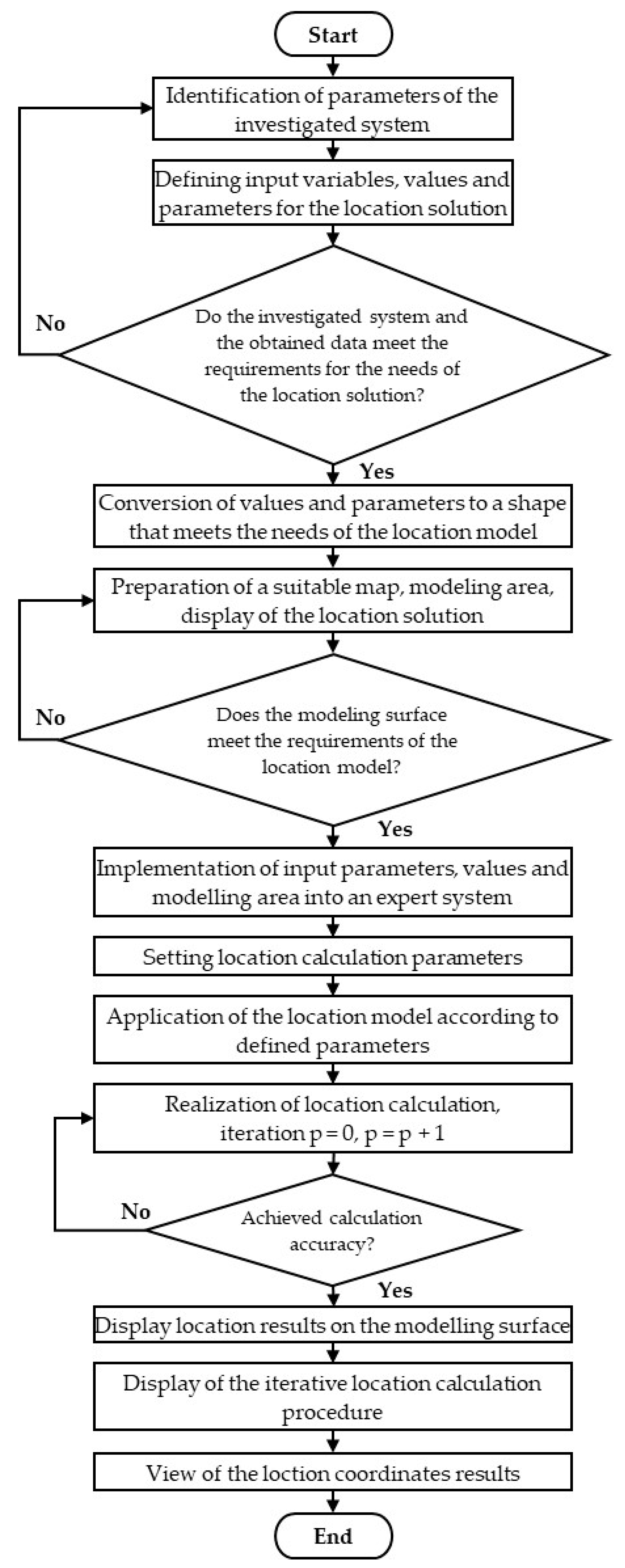
3. Materials and Methods
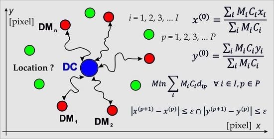
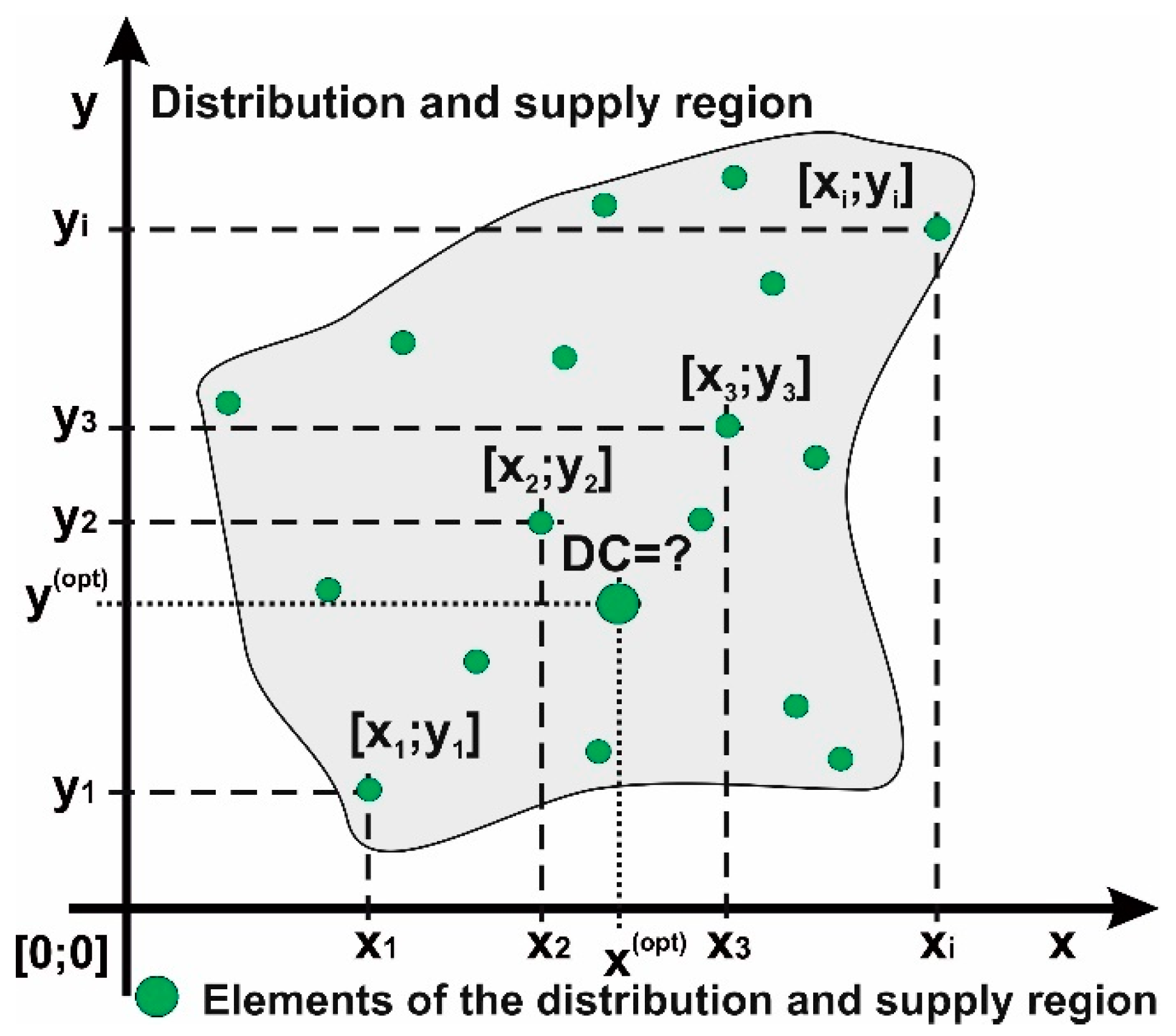
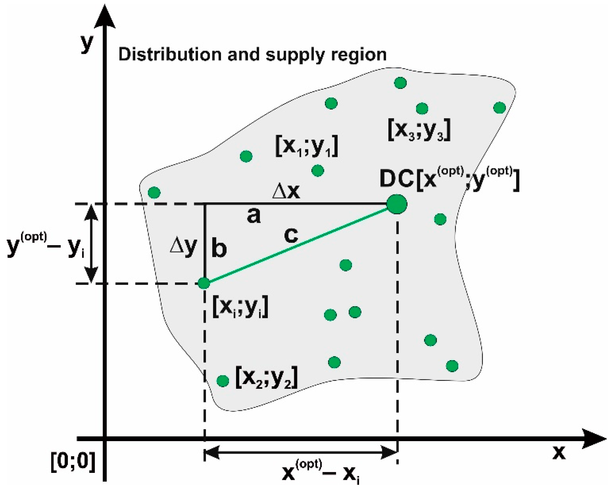
3.1. Problem Description
3.2. Mathematical Formulation
- -
- each point entering the calculation has fixed distribution costs, which are formed by the product of the transported quantity of material and the unit price for the transport of the material;
- -
- there is one common distribution centre for each point;
- -
- the distribution centre is responsible for carrying out supply and distribution;
- -
- the optimisation function depends on the transported quantity of material, the unit price per material, the distance between the point of receipt of the material and the point of dispatch.
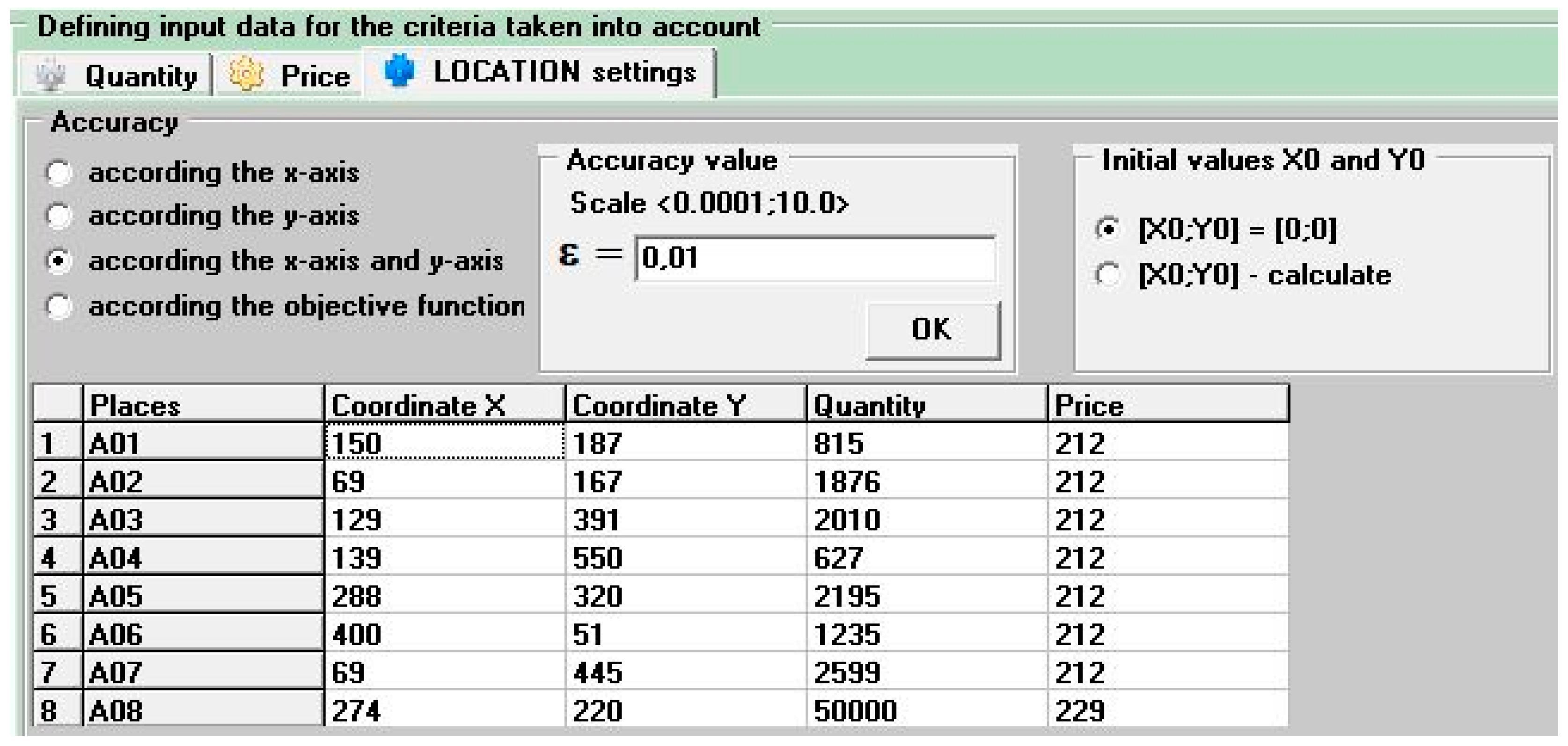
- based on the x-axis,
- based on the y-axis,
- based on the x- and y-axes simultaneously,
- based on the objective function change z,
- based on the change in the movement of the calculated coordinates—the calculation ends when the values of the calculated coordinates of two successive iterations do not change, e.g., the values of calculated coordinates are identical.
4. Results and Discussion
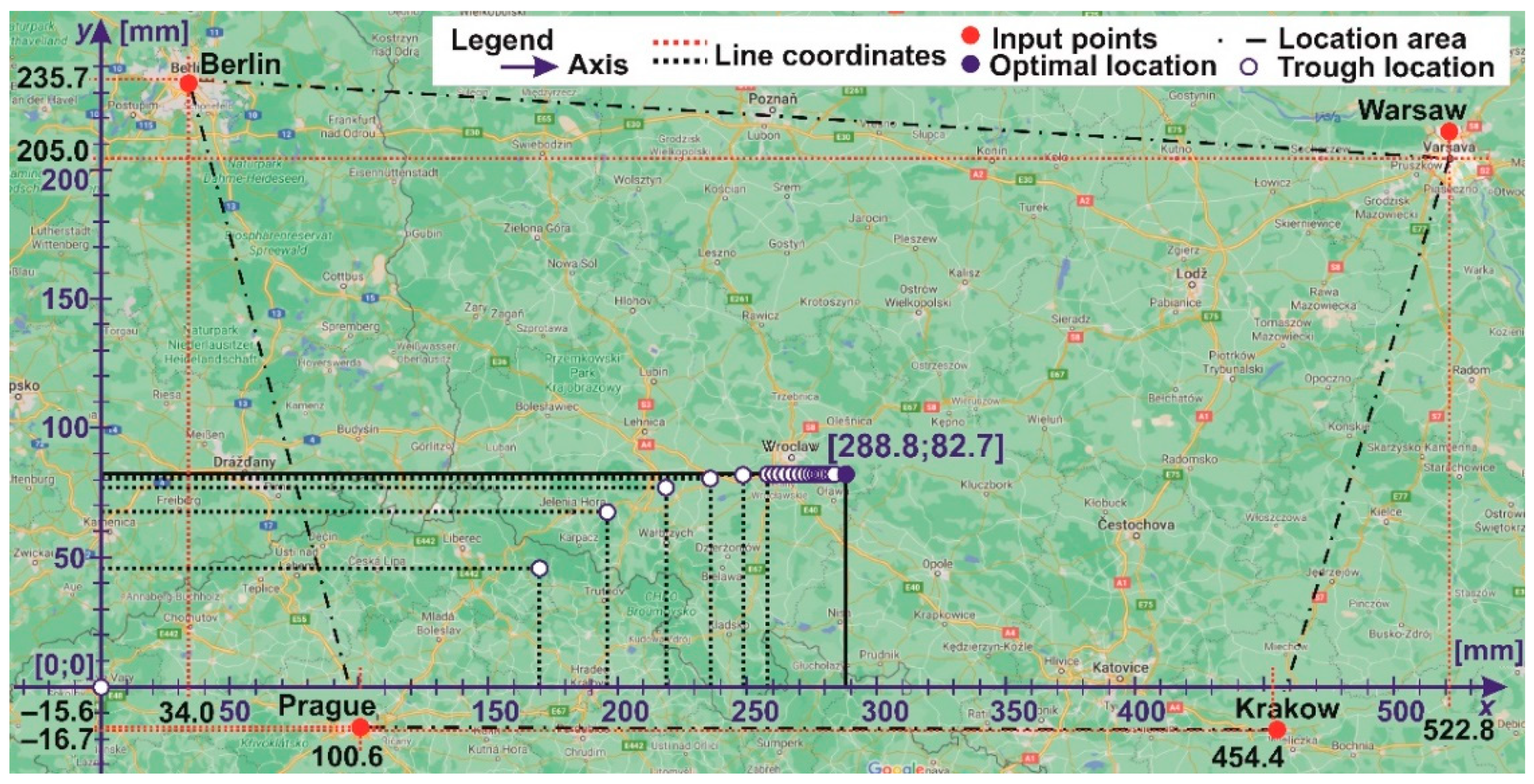
4.1. Location using Direct Distance, Cooper’s Iteration Method, Traditional Approach
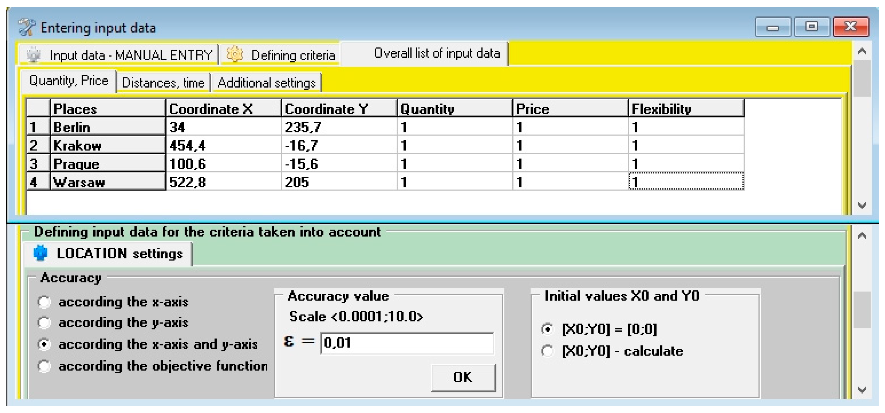
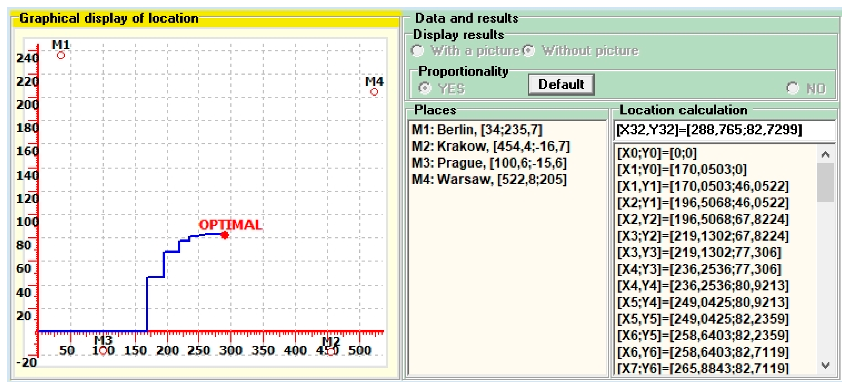
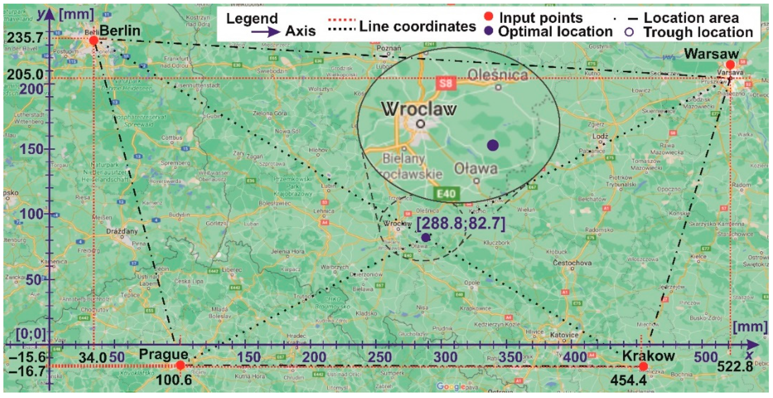
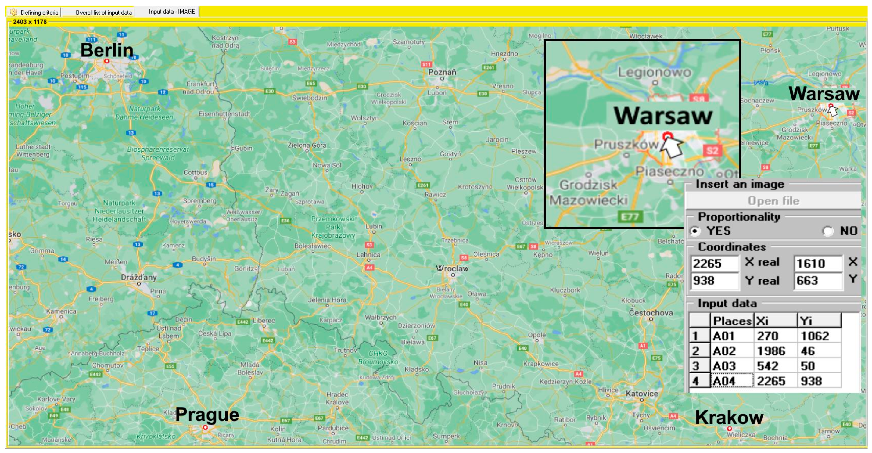
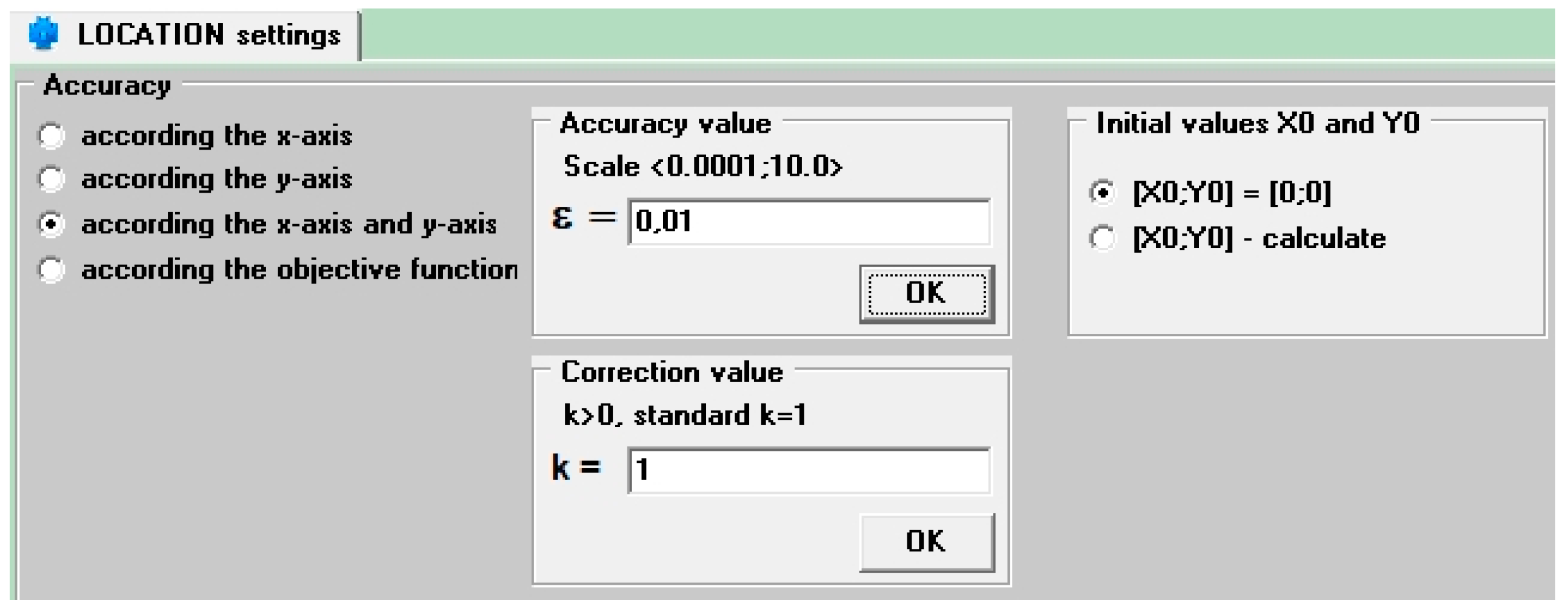
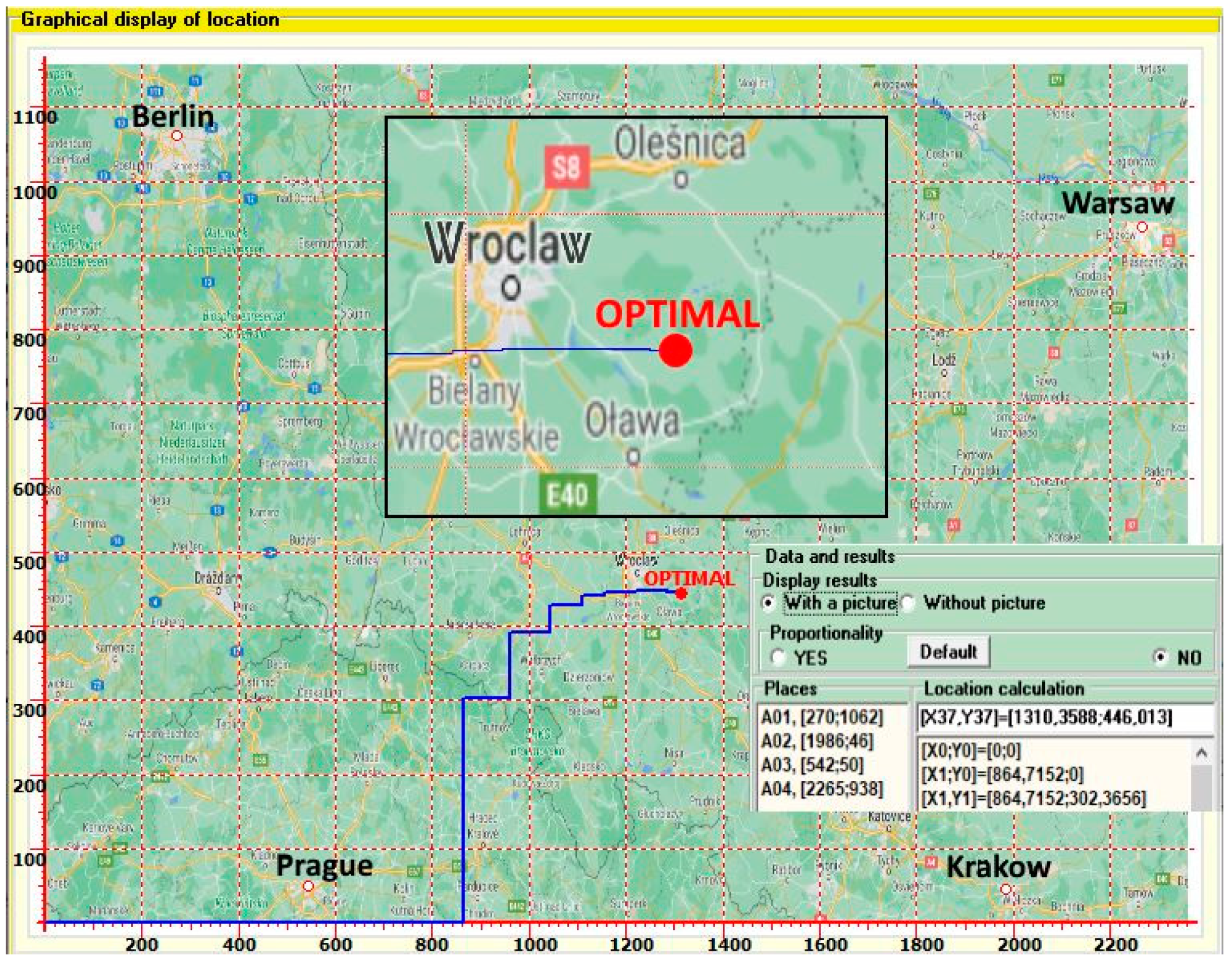
4.2. Location Using Computer-Aided Location Expert System
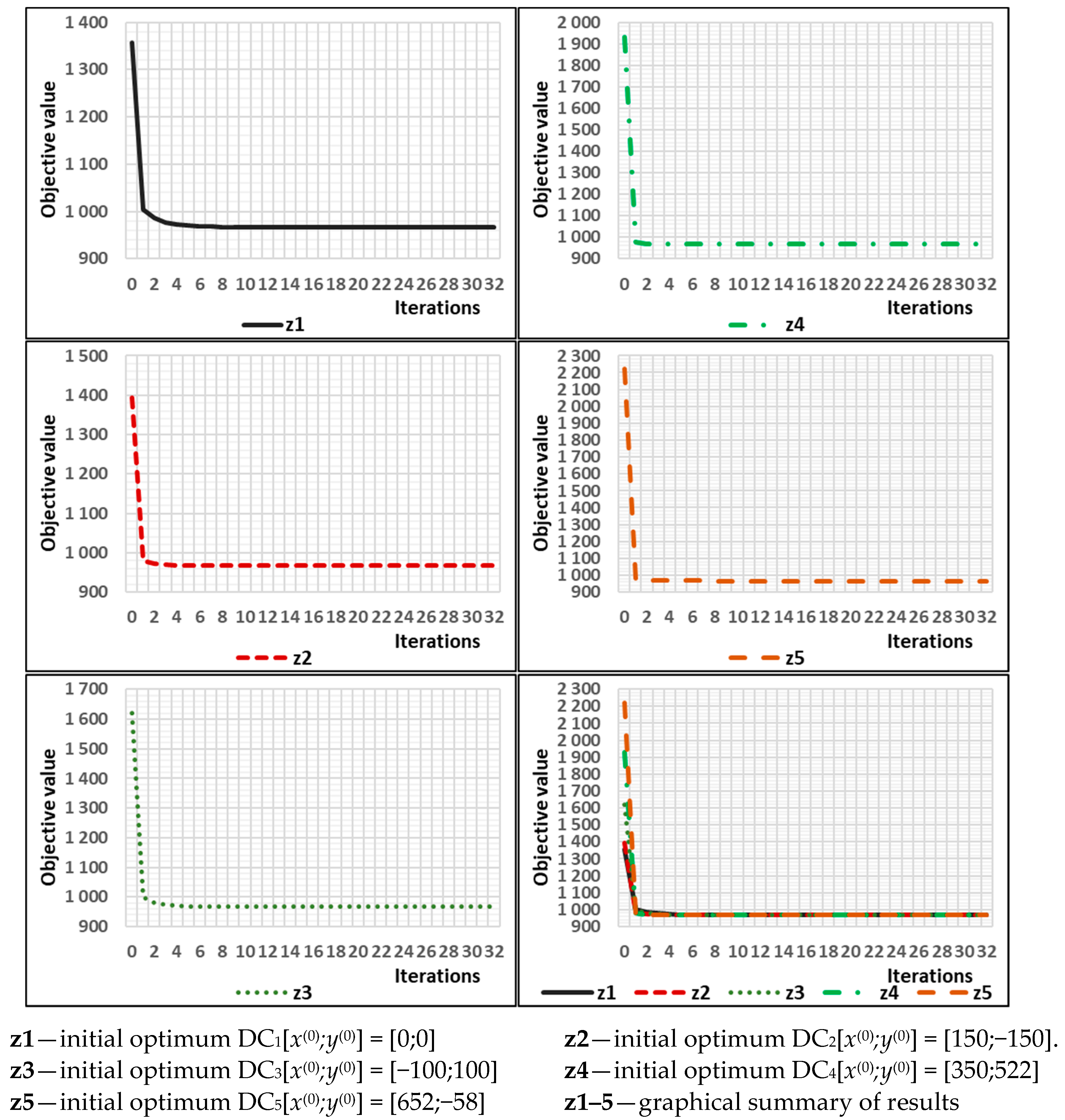
4.3. Location, Proof of Optimality
4.4. Location Using Computer-Aided Location Expert System, Case Study
4.5. Location, Case Study Proof of Optimality
5. Conclusions
Funding
Institutional Review Board Statement
Informed Consent Statement
Data Availability Statement
Acknowledgments
Conflicts of Interest
References
- Straka, M. Distribution and Supply Logistics; Cambridge Scholars Publishing: Newcastle upon Tyne, UK, 2019. [Google Scholar]
- Von Thünen, J.H. Der isolierte Staat (The Isolated State); Perthes: Hamburg, Germany, 1826. [Google Scholar]
- Launhardt, W. Die Bestimmung des zweckmässigsten Standortes einer gewerblichen Anlage. Z. Ver. Dtsch. Ing. 1882, 26, 106–115. [Google Scholar]
- Weber, A. Über den Standort der Industrien, Tübingen; University of Chicago Press: Chicago, IL, USA, 1909. [Google Scholar]
- Christaller, W. Die Zentralen Orte in Süddeutschland; Fischer: Berlin, Germany, 1933. [Google Scholar]
- Losch, A. The Economics of Location; Fischer: Berlin, Germany, 1940. [Google Scholar]
- Moses, L.N. Location and the Theory of Production. Q. J. Econ. 1958, 72, 259–606. [Google Scholar] [CrossRef]
- Beckmann, M.J. Location Theory; Random House: New York, NY, USA, 1968. [Google Scholar]
- Malindzak, D. Production Logistics I; Stroffek: Kosice, Slovakia, 1996. [Google Scholar]
- Straka, M. Distribution Logistics in Examples, 2nd ed.; FBERG TUKE: Kosice, Slovakia, 2012. [Google Scholar]
- Shavarani, S.M.; Mosallaeipour, S.; Golabi, M.; İzbirak, G. A congested capacitated multi-level fuzzy facility location problem: An efficient drone delivery system. Comput. Oper. Res. 2019, 108, 57–68. [Google Scholar] [CrossRef]
- Wen, M.; Lu, B.; Li, S.; Kang, R. Location and allocation problem for spare parts depots on integrated logistics support. J. Syst. Eng. Electron. 2019, 30, 1252–1259. [Google Scholar] [CrossRef]
- Barojas-Payán, E.; Sánchez-Partida, D.; Martínez-Flores, J.L.; Gibaja-Romero, D.E. Mathematical Model for Locating a Pre-Positioned Warehouse and for Calculating Inventory Levels. J. Disaster Res. 2019, 14, 649–666. [Google Scholar] [CrossRef]
- Mardani, A.; Jusoh, A.; Zavadskas, E.K. Fuzzy multiple criteria decision-making techniques and applications: Two decades review from 1994 to 2014. Expert Syst. Appl. 2015, 42, 4126–4148. [Google Scholar] [CrossRef]
- Chen, J.; Wang, J.; Baležentis, T.; Zagurskaitė, F.; Streimikiene, D.; Makutėnienė, D. Multicriteria Approach towards the Sustainable Selection of a Teahouse Location with Sensitivity Analysis. Sustainability 2018, 10, 2926. [Google Scholar] [CrossRef] [Green Version]
- Kolios, A.; Mytilinou, V.; Lozano-Minguez, E.; Salonitis, K. A Comparative Study of Multiple-Criteria Decision-Making Methods under Stochastic Inputs. Energies 2016, 9, 566. [Google Scholar] [CrossRef] [Green Version]
- Alnahhal, M.; Tabash, M.I.; Ahrens, D. Optimal selection of third-party logistics providers using integer programming: A case study of a furniture company storage and distribution. Ann. Oper. Res. 2021, 1–22. [Google Scholar] [CrossRef]
- Ni, W.; Shu, J.; Song, M.; Xu, D.; Zhang, K. A Branch-and-Price Algorithm for Facility Location with General Facility Cost Functions. INFORMS J. Comput. 2021, 33, 86–104. [Google Scholar] [CrossRef]
- Darmian, S.M.; Moazzeni, S.; Hvattum, L.M. Multi-objective sustainable location-districting for the collection of municipal solid waste: Two case studies. Comput. Ind. Eng. 2020, 150, 106965. [Google Scholar] [CrossRef]
- Eiselt, H.; Marianov, V. Location modeling for municipal solid waste facilities. Comput. Oper. Res. 2015, 62, 305–315. [Google Scholar] [CrossRef]
- Nouri, J.; Maghsoudlou, B.; Aboushahab, Z. Utilization multi attribute decision making models for spatial prioritization and environmental decision making in new towns. Int. J. Environ. Sci. Technol. 2013, 10, 443–454. [Google Scholar] [CrossRef] [Green Version]
- Bertola, N.J.; Smith, I.F. A methodology for measurement-system design combining information from static and dynamic excitations for bridge load testing. J. Sound Vib. 2019, 463, 114953. [Google Scholar] [CrossRef]
- Abdelbari, H.; Shafi, K. A System Dynamics Modeling Support System Based on Computational Intelligence. Systems 2019, 7, 47. [Google Scholar] [CrossRef] [Green Version]
- Chou, T.Y.; Hsu, C.L.; Chen, M.C. A fuzzy multi-criteria decision model for international tourist hotels location selection. Int. J. Hosp. Manag. 2008, 27, 293–301. [Google Scholar] [CrossRef]
- David, J.; Tuhý, T.; Jančíková, Z.K. Method for optimizing maintenance location within the industrial plant. Acta Logist. 2019, 6, 55–62. [Google Scholar] [CrossRef]
- Tönissen, D.D.; Arts, J.J.; Shen, Z.J. Maintenance Location Routing for Rolling Stock Under Line and Fleet Planning Uncertainty. Transp. Sci. 2019, 53, 1252–1270. [Google Scholar] [CrossRef]
- Bhattacharya, B.K.; De, M.; Nandy, S.C.; Roy, S. Constant work-space algorithms for facility location problems. Discret. Appl. Math. 2020, 283, 456–472. [Google Scholar] [CrossRef]
- Zhang, D.; Yang, S.; Li, S.; Fan, J.; Ji, B. Integrated Optimization of the Location–Inventory Problem of Maintenance Component Distribution for High-Speed Railway Operations. Sustainability 2020, 12, 5447. [Google Scholar] [CrossRef]
- Malec, M.; Benalcazar, P.; Kaszyński, P. Optimal location of gas network maintenance centres: A case study from Poland. J. Nat. Gas Sci. Eng. 2020, 83, 103569. [Google Scholar] [CrossRef]
- Sánchez-Sierra, S.T.; Caballero-Morales, S.O.; Sánchez-Partida, D.; Martínez-Flores, J.L. Facility location model with inventory transportation and management costs. Acta Logist. 2018, 5, 79–86. [Google Scholar] [CrossRef]
- Karatas, M.; Kutanoglu, E. Joint optimization of location, inventory, and condition-based replacement decisions in service parts logistics. IISE Trans. 2021, 53, 246–271. [Google Scholar] [CrossRef]
- Yuchi, Q.; Wang, N.; He, Z.; Chen, H. Hybrid heuristic for the location-inventory-routing problem in closed-loop supply chain. Int. Trans. Oper. Res. 2021, 28, 1265–1295. [Google Scholar] [CrossRef]
- Wu, W.; Zhou, W.; Lin, Y.; Xie, Y.; Jin, W. A hybrid metaheuristic algorithm for location inventory routing problem with time windows and fuel consumption. Expert Syst. Appl. 2020, 166, 114034. [Google Scholar] [CrossRef]
- Ehsanifar, M.; Wood, D.A.; Babaie, A. UTASTAR method and its application in multi-criteria warehouse location selection. Oper. Manag. Res. 2020, 1–14. [Google Scholar] [CrossRef]
- Moradlou, H.; Reefke, H.; Skipworth, H.; Roscoe, S. Geopolitical disruptions and the manufacturing location decision in multinational company supply chains: A Delphi study on Brexit. Int. J. Oper. Prod. Manag. 2021, 41, 102–130. [Google Scholar] [CrossRef]
- Huo, D.; Chaudhry, H.R. Using machine learning for evaluating global expansion location decisions: An analysis of Chinese manufacturing sector. Technol. Forecast. Soc. Chang. 2021, 163, 120436. [Google Scholar] [CrossRef]
- Shafiee-Gol, S.; Kia, R.; Kazemi, M.; Tavakkoli-Moghaddam, R.; Darmian, S.M. A mathematical model to design dynamic cellular manufacturing systems in multiple plants with production planning and location–allocation decisions. Soft Comput. 2021, 25, 3931–3954. [Google Scholar] [CrossRef]
- Woo, Y.; Kim, E. Analysing location choices of small and large enterprises of electronics-manufacturing industry in Korea. Appl. Econ. Lett. 2020, 27, 1–6. [Google Scholar] [CrossRef]
- Theyel, G.; Hofmann, K.H. Manufacturing location decisions and organizational agility. Multinatl. Bus. Rev. 2021, 29, 166–188. [Google Scholar] [CrossRef]
- Todorov, T.; Stoinov, J. Expert System for Milk and Animal Monitoring. Int. J. Adv. Comput. Sci. Appl. 2019, 10, 25–30. [Google Scholar] [CrossRef]
- Shah, D.S.; Jha, D.K.; Gurram, S.; Suñé-Pou, M.; Garcia-Montoya, E.; Amin, P.D. A new SeDeM-SLA expert system for screening of solid carriers for the preparation of solidified liquids: A case of citronella oil. Powder Technol. 2021, 382, 605–618. [Google Scholar] [CrossRef]
- Rogulj, K.; Pamuković, J.K.; Jajac, N. Knowledge-Based Fuzzy Expert System to the Condition Assessment of Historic Road Bridges. Appl. Sci. 2021, 11, 1021. [Google Scholar] [CrossRef]
- Dattachaudhuri, A.; Biswas, S.K.; Chakraborty, M.; Sarkar, S. A transparent rule-based expert system using neural network. Soft Comput. 2021, 1–14. [Google Scholar] [CrossRef]
- Zhao, L.; Tao, W.; Wang, G.; Wang, L.; Liu, G. Intelligent anti-corrosion expert system based on big data analysis. Anti-Corrosion Methods Mater. 2021, 68, 17–28. [Google Scholar] [CrossRef]
- Choi, D.; Lee, H.; Bok, K.; Yoo, J. Design and implementation of an academic expert system through big data analysis. J. Supercomput. 2021, 1–25. [Google Scholar] [CrossRef]
- Sarkar, J.; Al Faruque, A.; Mondal, M.S. Modeling the seam strength of denim garments by using fuzzy expert system. J. Eng. Fibers Fabr. 2021, 16, 1–10. [Google Scholar] [CrossRef]
- Nuhu, B.K.; Aliyu, I.; Adegboye, M.A.; Ryu, J.K.; Olaniyi, O.M.; Lim, C.G. Distributed network-based structural health monitoring expert system. Build. Res. Inf. 2021, 49, 144–159. [Google Scholar] [CrossRef]
- Gong, K.; Zhang, L.; Ni, D.; Li, H.; Xu, M.; Wang, Y.; Dong, Y. An expert system to discover key congestion points for urban traffic. Expert Syst. Appl. 2020, 158, 113544. [Google Scholar] [CrossRef]
- Shokouhyar, S.; Seifhashemi, S.; Siadat, H.; Ahmadi, M.M. Implementing a fuzzy expert system for ensuring information technology supply chain. Expert Syst. 2019, 36, e12339. [Google Scholar] [CrossRef] [Green Version]
- Hsu, Y.Y.; Lu, F.C.; Chien, Y.; Liu, J.; Lin, J.; Yu, P.; Kuo, R. An expert system for locating distribution system faults. IEEE Trans. Power Deliv. 1991, 6, 366–372. [Google Scholar] [CrossRef]
- Kim, H.; Ko, Y.; Shon, S. An Expert System for the Electric Power Distribution System Design. IFAC Proc. Vol. 1989, 22, 483–488. [Google Scholar] [CrossRef]
- Tang, D.; Shi, J.; Wang, W. Intelligent expert systems for location planning. Appl. Math. Inf. Sci. 2015, 9, 1611–1621. [Google Scholar]
- Bachár, M.; Makyšová, H.; Loučanová, E.; Olšiaková, M.; Nosáľová, M.; Štofková-Repková, K. Evaluation of the impact of intelligent logistics elements on the efficiency of functioning internal logistics processes. Acta Technol. 2019, 5, 55–58. [Google Scholar] [CrossRef]
- Warszawski, A.; Peled, N. An Expert System for Crane Selection and Location. In Proceedings of the 4th International Symposium on Automation and Robotics in Construction, Haifa, Israel, 22–25 June 1987; pp. 64–75. [Google Scholar]
- Teng, M.H. Application of multicriteria decision making for site selection of restaurants: Case study of Pao-San restaurant. J. Living Sci. 2000, 6, 47–62. [Google Scholar]
- Kahfi, A.; Seyed-Hosseni, S.M.; Tavakoli-Moghadam, R. A robust optimisation approach for a multi-period location-arc routing problem with time windows: A case study of a bank. Int. J. Nonlinear Analysis Appl. 2021, 12, 157–173. [Google Scholar] [CrossRef]
- Lodi, A.; Mossina, L.; Rachelson, E. Learning to handle parameter perturbations in Combinatorial Optimization: An application to facility location. EURO J. Transp. Logist. 2020, 9, 100023. [Google Scholar] [CrossRef]
- Zavadsky, J.; Kozarova, M.; Vinczeova, M.; Tuckova, Z.; Krivosudska, J. How organisational innovations help managers to improve quality of their work: An empirical study. Int. J. Qual. Res. 2018, 12, 905–924. [Google Scholar] [CrossRef]
- Wicher, P.; Zapletal, F.; Lenort, R. Sustainability performance assessment of industrial corporation using Fuzzy Analytic Network Process. J. Clean. Prod. 2019, 241, 118132. [Google Scholar] [CrossRef]
- Alizadeh, M.; Amiri-Aref, M.; Mustafee, N.; Matilal, S. A robust stochastic Casualty Collection Points location problem. Eur. J. Oper. Res. 2019, 279, 965–983. [Google Scholar] [CrossRef]
- Samolejova, A.; Feliks, J.; Lenort, R.; Besta, P. A hybrid decision support system for iron ore supply. Metalurgija 2012, 51, 91–93. [Google Scholar]
- Antoniou, F.; Aretoulis, G. A multi-criteria decision-making support system for choice of method of compensation for highway construction contractors in Greece. Int. J. Constr. Manag. 2018, 19, 492–508. [Google Scholar] [CrossRef]
- Phung, X.L.; Truong, H.S.; Bui, N.T. Expert System Based on Integrated Fuzzy AHP for Automatic Cutting Tool Selection. Appl. Sci. 2019, 9, 4308. [Google Scholar] [CrossRef] [Green Version]
- Kim, E.W.; Kim, S. Optimum Location Analysis for an Infrastructure Maintenance Depot in Urban Railway Networks. KSCE J. Civ. Eng. 2021, 1–12. [Google Scholar] [CrossRef]
- Wang, C.N.; Hsueh, M.H.; Lin, D.F. Hydrogen Power Plant Site Selection Under Fuzzy Multicriteria Decision-Making (FMCDM) Environment Conditions. Symmetry 2019, 11, 596. [Google Scholar] [CrossRef] [Green Version]
- Ali, L.; Khan, S.U.; Golilarz, N.A.; Yakubu, I.; Qasim, I.; Noor, A.; Nour, R. A Feature-Driven Decision Support System for Heart Failure Prediction Based on χ2 Statistical Model and Gaussian Naive Bayes. Comput. Math. Methods Med. 2019, 2019, 6314328. [Google Scholar] [CrossRef] [PubMed] [Green Version]
- Mosallaeipour, S.; Shavarani, S.M.; Steens, C.; Eros, A. A robust expert decision support system for making real estate location decisions, a case of investor-developer-user organization in industry 4.0 era. J. Corp. Real Estate 2019, 22, 21–47. [Google Scholar] [CrossRef]
- Wulandari, N.; Abdullah, A.G.; Kustiawan, I. Development of an application of critical thinking skills tools using fuzzy expert system. J. Eng. Sci. Technol. 2019, 14, 3073–3086. [Google Scholar]
- Saderova, J.; Rosova, A.; Behunova, A.; Behun, M.; Sofranko, M.; Khouri, S. Case study: The simulation modelling of selected activity in a warehouse operation. Wirel. Netw. 2021, 7, 1–10. [Google Scholar] [CrossRef]
- Wang, C.N.; Van Thanh, N.; Su, C.C. The Study of a Multicriteria Decision Making Model for Wave Power Plant Location Selection in Vietnam. Processes 2019, 7, 650. [Google Scholar] [CrossRef] [Green Version]
- Cooper, L. Location-Allocation Problems. Oper. Res. 1963, 11, 331–343. [Google Scholar] [CrossRef]
- Straka, M. Distribution Logistics as a Component Part of Micrologistics Model of an Enterprise. Habilitation Thesis, Technical University of Ostrava, Ostrava, Czech Republic, 2007. [Google Scholar]


| Places | xi | yi | Mi | Ci |
|---|---|---|---|---|
| Berlin | 34.0 | 235.7 | 1 | 1.0 |
| Krakow | 454.4 | −16.7 | 1 | 1.0 |
| Prague | 100.6 | −15.6 | 1 | 1.0 |
| Warsaw | 522.8 | 205.0 | 1 | 1.0 |
| DC[x(0);y(0)] | 0.0 | 0.0 | ||
| ε | 0.01 | |||
| DC[x(opt);y(opt)] | ? | ? |
| Hi | Ai | Xi | Ri | Bi | Yi | x(i) | y(i) | |
|---|---|---|---|---|---|---|---|---|
| 0.0 | 0.0 | [x(0);y(0)] | ||||||
| −3.06127 | 0.01800 | −170.05033 | −1.09075 | 0.02368 | −46.05223 | 170.1 | 46.1 | [x(1);y(1)] |
| −0.55747 | 0.02107 | −26.45652 | −0.42012 | 0.01930 | −21.77017 | 196.5 | 67.8 | [x(2);y(2)] |
| −0.42208 | 0.01866 | −22.62340 | −0.16977 | 0.01790 | −9.48359 | 219.1 | 77.3 | [x(3);y(3)] |
| −0.30355 | 0.01773 | −17.12337 | −0.06281 | 0.01737 | −3.61537 | 236.3 | 80.9 | [x(4);y(4)] |
| −0.22150 | 0.01732 | −12.78887 | −0.02254 | 0.01715 | −1.31460 | 249.0 | 82.2 | [x(5);y(5)] |
| −0.16441 | 0.01713 | −9.59778 | −0.00811 | 0.01705 | −0.47596 | 258.6 | 82.7 | [x(6);y(6)] |
| −0.12345 | 0.01704 | −7.24399 | −0.00282 | 0.01701 | −0.16586 | 265.9 | 82.9 | [x(7);y(7)] |
| −0.09333 | 0.01700 | −5.48856 | −0.00077 | 0.01699 | −0.04525 | 271.4 | 82.9 | [x(8);y(8)] |
| −0.07082 | 0.01699 | −4.16783 | 0.00005 | 0.01699 | 0.00311 | 275.5 | 82.9 | [x(9);y(9)] |
| −0.05384 | 0.01699 | −3.16867 | 0.00037 | 0.01699 | 0.02152 | 278.7 | 82.9 | [x(10);y(10)] |
| −0.04097 | 0.01699 | −2.41044 | 0.00045 | 0.01700 | 0.02676 | 281.1 | 82.9 | [x(11);y(11)] |
| −0.03118 | 0.01700 | −1.83410 | 0.00045 | 0.01701 | 0.02619 | 283.0 | 82.8 | [x(12);y(12)] |
| −0.02374 | 0.01701 | −1.39567 | 0.00040 | 0.01701 | 0.02325 | 284.3 | 82.8 | [x(13);y(13)] |
| −0.01807 | 0.01701 | −1.06203 | 0.00033 | 0.01702 | 0.01960 | 285.4 | 82.8 | [x(14);y(14)] |
| −0.01375 | 0.01702 | −0.80811 | 0.00027 | 0.01702 | 0.01602 | 286.2 | 82.8 | [x(15);y(15)] |
| −0.01047 | 0.01702 | −0.61487 | 0.00022 | 0.01703 | 0.01283 | 286.8 | 82.8 | [x(16);y(16)] |
| −0.00797 | 0.01703 | −0.46780 | 0.00017 | 0.01703 | 0.01013 | 287.3 | 82.8 | [x(17);y(17)] |
| −0.00606 | 0.01703 | −0.35590 | 0.00013 | 0.01703 | 0.00792 | 287.7 | 82.8 | [x(18);y(18)] |
| −0.00461 | 0.01703 | −0.27075 | 0.00010 | 0.01703 | 0.00615 | 287.9 | 82.7 | [x(19);y(19)] |
| −0.00351 | 0.01703 | −0.20597 | 0.00008 | 0.01703 | 0.00475 | 288.1 | 82.7 | [x(20);y(20)] |
| −0.00267 | 0.01703 | −0.15668 | 0.00006 | 0.01704 | 0.00365 | 288.3 | 82.7 | [x(21);y(21)] |
| −0.00203 | 0.01704 | −0.11918 | 0.00005 | 0.01704 | 0.00280 | 288.4 | 82.7 | [x(22);y(22)] |
| −0.00154 | 0.01704 | −0.09066 | 0.00004 | 0.01704 | 0.00215 | 288.5 | 82.7 | [x(23);y(23)] |
| −0.00117 | 0.01704 | −0.06896 | 0.00003 | 0.01704 | 0.00164 | 288.6 | 82.7 | [x(24);y(24)] |
| −0.00089 | 0.01704 | −0.05246 | 0.00002 | 0.01704 | 0.00125 | 288.6 | 82.7 | [x(25);y(25)] |
| −0.00068 | 0.01704 | −0.03990 | 0.00002 | 0.01704 | 0.00096 | 288.7 | 82.7 | [x(26);y(26)] |
| −0.00052 | 0.01704 | −0.03035 | 0.00001 | 0.01704 | 0.00073 | 288.7 | 82.7 | [x(27);y(27)] |
| −0.00039 | 0.01704 | −0.02309 | 0.00001 | 0.01704 | 0.00056 | 288.7 | 82.7 | [x(28);y(28)] |
| −0.00030 | 0.01704 | −0.01756 | 0.00001 | 0.01704 | 0.00042 | 288.7 | 82.7 | [x(29);y(29)] |
| −0.00023 | 0.01704 | −0.01336 | 0.00001 | 0.01704 | 0.00032 | 288.7 | 82.7 | [x(30);y(30)] |
| −0.00017 | 0.01704 | −0.01016 | 0.00000 | 0.01704 | 0.00024 | 288.8 | 82.7 | [x(31);y(31)] |
| −0.00013 | 0.01704 | −0.00773 | 0.00000 | 0.01704 | 0.00019 | 288.8 | 82.7 | [x(32);y(32)] |
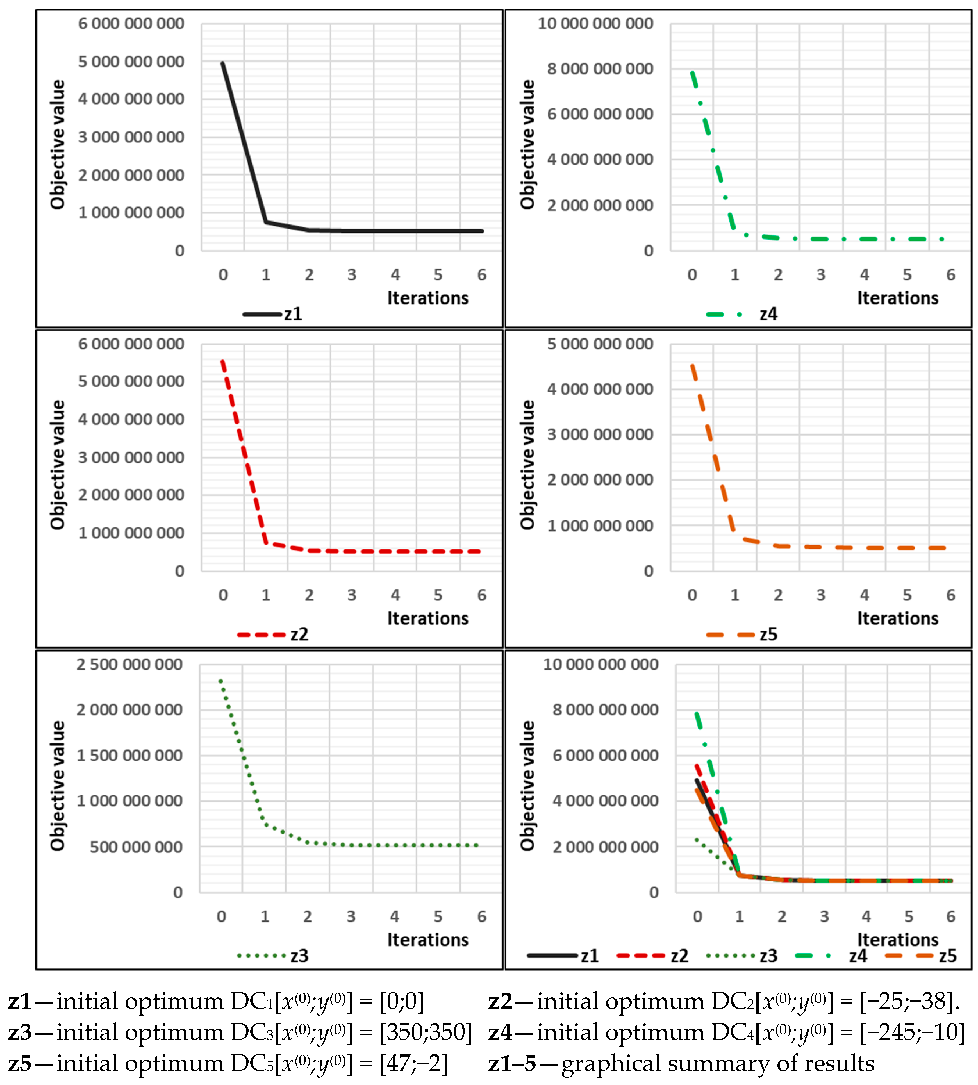
| x(i) | y(i) | z1 | x(i) | y(i) | z2 | x(i) | y(i) | z3 | x(i) | y(i) | z4 | x(i) | y(i) | z5 | |
|---|---|---|---|---|---|---|---|---|---|---|---|---|---|---|---|
| 0 | 0 | 0 | 1356.2 | 150 | −150 | 1393.1 | −100 | 100 | 1620.4 | 350 | 522 | 1928.8 | 652 | −58 | 1732.2 |
| 1 | 170.1 | 46.1 | 1004.4 | 219.9 | 61.2 | 979.3 | 173.7 | 86.8 | 997.7 | 292.8 | 124.2 | 977.6 | 366.7 | 49.7 | 985.4 |
| 2 | 196.5 | 67.8 | 986.1 | 235.6 | 76.7 | 972.8 | 206.5 | 82.5 | 981.3 | 291.0 | 92.8 | 967.4 | 349.7 | 70.0 | 975.4 |
| 3 | 219.1 | 77.3 | 977.0 | 248.3 | 81.1 | 970.1 | 227.6 | 82.0 | 974.5 | 290.3 | 85.2 | 966.8 | 335.0 | 77.5 | 971.3 |
| 4 | 236.3 | 80.9 | 972.4 | 258.1 | 82.4 | 968.6 | 242.8 | 82.4 | 971.1 | 289.9 | 83.3 | 966.7 | 323.7 | 80.3 | 969.3 |
| 5 | 249.0 | 82.2 | 969.9 | 265.5 | 82.8 | 967.8 | 253.9 | 82.7 | 969.2 | 289.6 | 82.9 | 966.7 | 315.2 | 81.4 | 968.2 |
| 6 | 258.6 | 82.7 | 968.6 | 271.0 | 82.9 | 967.3 | 262.3 | 82.9 | 968.1 | 289.4 | 82.7 | 966.7 | 308.8 | 81.9 | 967.5 |
| 7 | 265.9 | 82.9 | 967.8 | 275.3 | 82.9 | 967.1 | 268.7 | 82.9 | 967.5 | 289.3 | 82.7 | 966.7 | 304.0 | 82.2 | 967.2 |
| 8 | 271.4 | 82.9 | 967.3 | 278.5 | 82.9 | 966.9 | 273.5 | 82.9 | 967.2 | 289.2 | 82.7 | 966.7 | 300.3 | 82.3 | 967.0 |
| 9 | 275.5 | 82.9 | 967.1 | 281.0 | 82.9 | 966.8 | 277.2 | 82.9 | 967.0 | 289.1 | 82.7 | 966.7 | 297.5 | 82.5 | 966.9 |
| 10 | 278.7 | 82.9 | 966.9 | 282.8 | 82.8 | 966.8 | 279.9 | 82.9 | 966.9 | 289.0 | 82.7 | 966.7 | 295.4 | 82.5 | 966.8 |
| 11 | 281.1 | 82.9 | 966.8 | 284.3 | 82.8 | 966.7 | 282.1 | 82.9 | 966.8 | 288.9 | 82.7 | 966.7 | 293.8 | 82.6 | 966.8 |
| 12 | 283.0 | 82.8 | 966.8 | 285.3 | 82.8 | 966.7 | 283.7 | 82.8 | 966.8 | 288.9 | 82.7 | 966.7 | 292.6 | 82.6 | 966.7 |
| 13 | 284.3 | 82.8 | 966.7 | 286.2 | 82.8 | 966.7 | 284.9 | 82.8 | 966.7 | 288.9 | 82.7 | 966.7 | 291.7 | 82.7 | 966.7 |
| 14 | 285.4 | 82.8 | 966.7 | 286.8 | 82.8 | 966.7 | 285.8 | 82.8 | 966.7 | 288.9 | 82.7 | 966.7 | 291.0 | 82.7 | 966.7 |
| 15 | 286.2 | 82.8 | 966.7 | 287.3 | 82.8 | 966.7 | 286.5 | 82.8 | 966.7 | 288.8 | 82.7 | 966.7 | 290.5 | 82.7 | 966.7 |
| 16 | 286.8 | 82.8 | 966.7 | 287.6 | 82.8 | 966.7 | 287.1 | 82.8 | 966.7 | 288.8 | 82.7 | 966.7 | 290.1 | 82.7 | 966.7 |
| 17 | 287.3 | 82.8 | 966.7 | 287.9 | 82.7 | 966.7 | 287.5 | 82.8 | 966.7 | 288.8 | 82.7 | 966.7 | 289.8 | 82.7 | 966.7 |
| 18 | 287.7 | 82.8 | 966.7 | 288.1 | 82.7 | 966.7 | 287.8 | 82.8 | 966.7 | 288.8 | 82.7 | 966.7 | 289.5 | 82.7 | 966.7 |
| 19 | 287.9 | 82.7 | 966.7 | 288.3 | 82.7 | 966.7 | 288.0 | 82.7 | 966.7 | 288.8 | 82.7 | 966.7 | 289.4 | 82.7 | 966.7 |
| 20 | 288.1 | 82.7 | 966.7 | 288.4 | 82.7 | 966.7 | 288.2 | 82.7 | 966.7 | 288.8 | 82.7 | 966.7 | 289.2 | 82.7 | 966.7 |
| 21 | 288.3 | 82.7 | 966.7 | 288.5 | 82.7 | 966.7 | 288.4 | 82.7 | 966.7 | 288.8 | 82.7 | 966.7 | 289.1 | 82.7 | 966.7 |
| 22 | 288.4 | 82.7 | 966.7 | 288.6 | 82.7 | 966.7 | 288.5 | 82.7 | 966.7 | 288.8 | 82.7 | 966.7 | 289.0 | 82.7 | 966.7 |
| 23 | 288.5 | 82.7 | 966.7 | 288.6 | 82.7 | 966.7 | 288.5 | 82.7 | 966.7 | 288.8 | 82.7 | 966.7 | 289.0 | 82.7 | 966.7 |
| 24 | 288.6 | 82.7 | 966.7 | 288.7 | 82.7 | 966.7 | 288.6 | 82.7 | 966.7 | 288.8 | 82.7 | 966.7 | 288.9 | 82.7 | 966.7 |
| 25 | 288.6 | 82.7 | 966.7 | 288.7 | 82.7 | 966.7 | 288.6 | 82.7 | 966.7 | 288.8 | 82.7 | 966.7 | 288.9 | 82.7 | 966.7 |
| 26 | 288.7 | 82.7 | 966.7 | 288.7 | 82.7 | 966.7 | 288.7 | 82.7 | 966.7 | 288.8 | 82.7 | 966.7 | 288.9 | 82.7 | 966.7 |
| 27 | 288.7 | 82.7 | 966.7 | 288.7 | 82.7 | 966.7 | 288.7 | 82.7 | 966.7 | 288.8 | 82.7 | 966.7 | 288.9 | 82.7 | 966.7 |
| 28 | 288.7 | 82.7 | 966.7 | 288.7 | 82.7 | 966.7 | 288.7 | 82.7 | 966.7 | 288.8 | 82.7 | 966.7 | 288.8 | 82.7 | 966.7 |
| 29 | 288.7 | 82.7 | 966.7 | 288.8 | 82.7 | 966.7 | 288.7 | 82.7 | 966.7 | 288.8 | 82.7 | 966.7 | 288.8 | 82.7 | 966.7 |
| 30 | 288.7 | 82.7 | 966.7 | 288.8 | 82.7 | 966.7 | 288.8 | 82.7 | 966.7 | 288.8 | 82.7 | 966.7 | 288.8 | 82.7 | 966.7 |
| 31 | 288.8 | 82.7 | 966.7 | 288.8 | 82.7 | 966.7 | 288.8 | 82.7 | 966.7 | 288.8 | 82.7 | 966.7 | 288.8 | 82.7 | 966.7 |
| 32 | 288.8 | 82.7 | 966.7 | 288.8 | 82.7 | 966.7 | 288.8 | 82.7 | 966.7 | 288.8 | 82.7 | 966.7 | 288.8 | 82.7 | 966.7 |
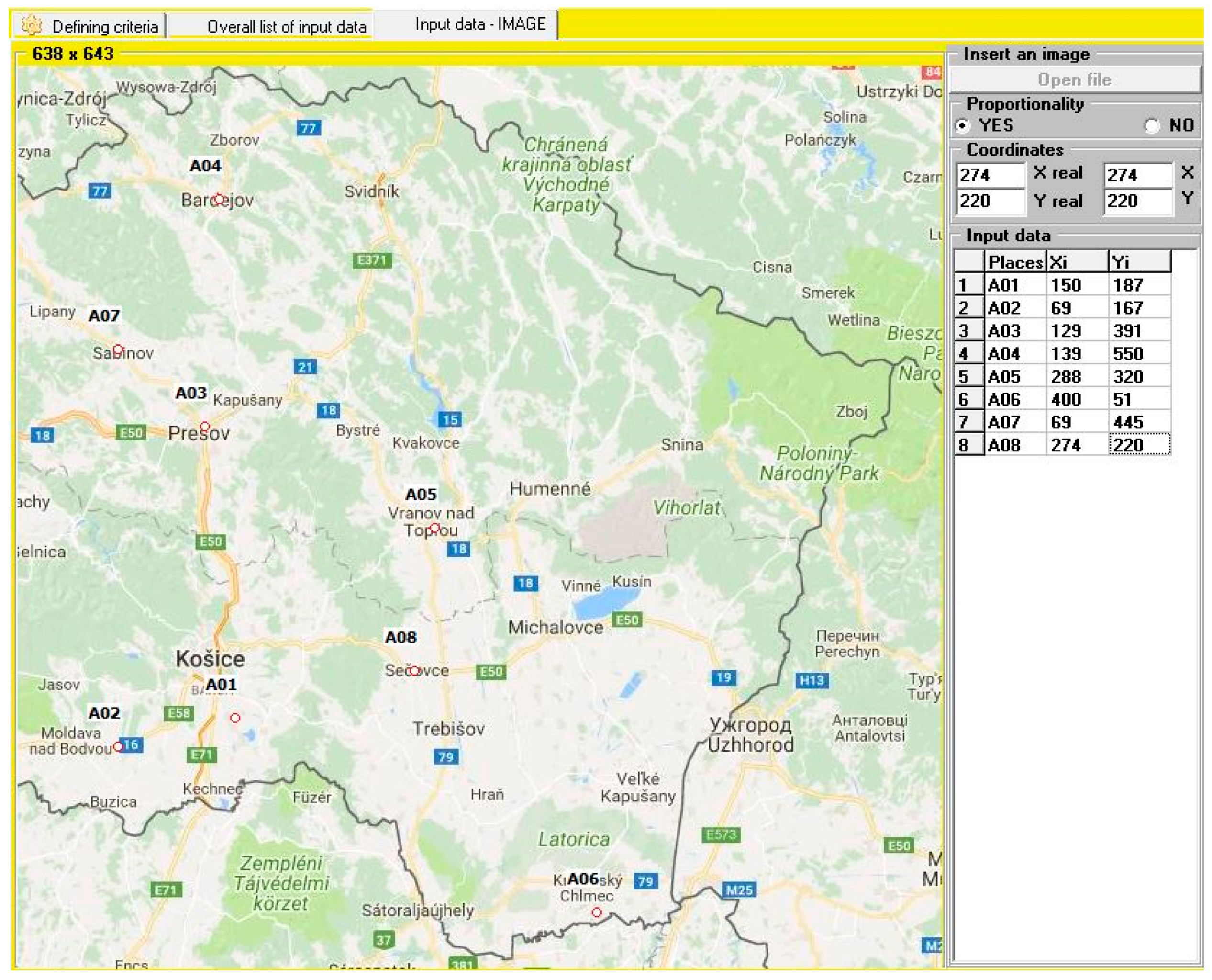
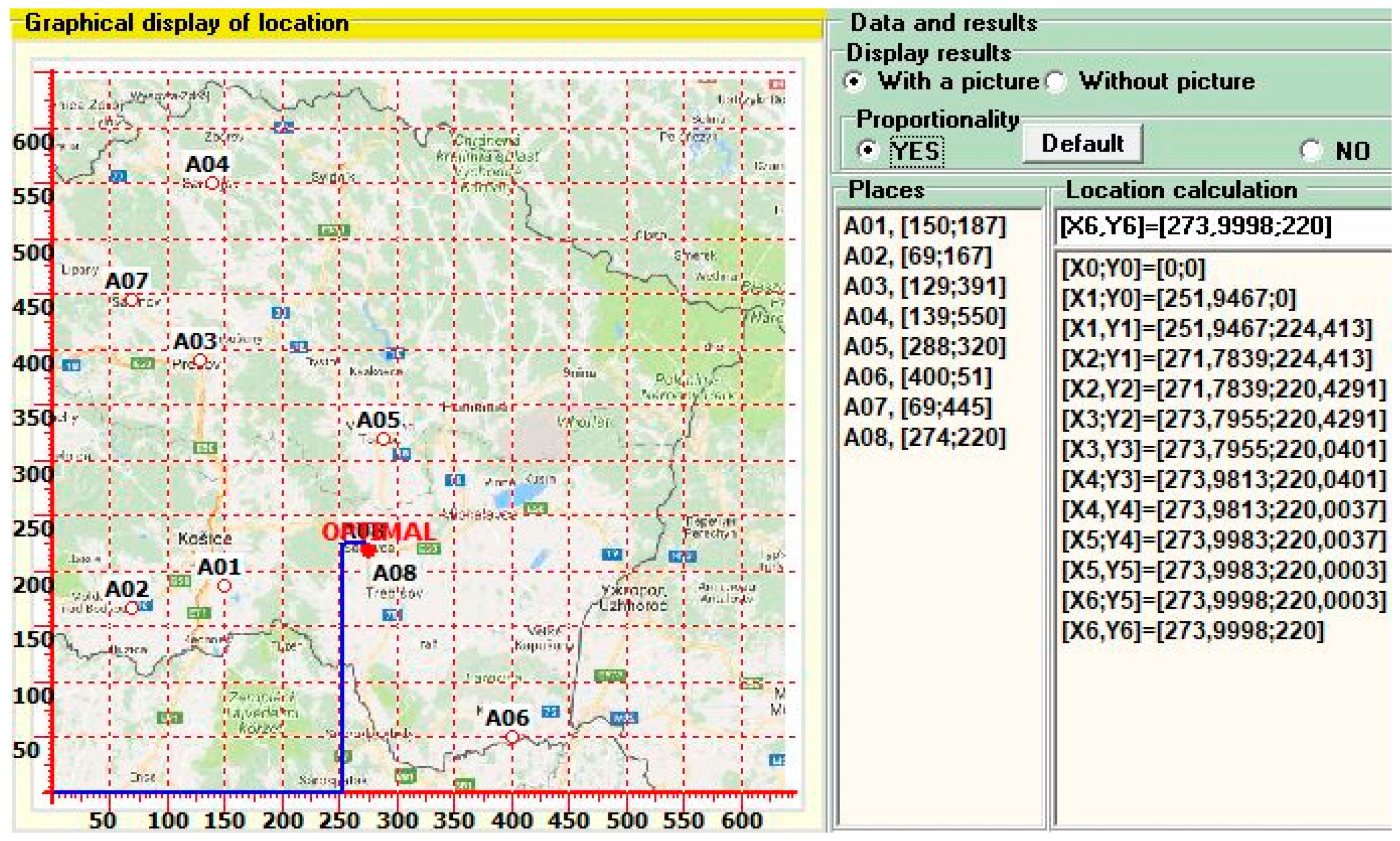
| Places of Supply | Coordinates | ||||
|---|---|---|---|---|---|
| xi | yi | Mi [t] | Ci [EUR/t] | ||
| Cana | A01 | 150 | 187 | 815 | 212 |
| Cecejovce | A02 | 69 | 167 | 1876 | 212 |
| Presov | A03 | 129 | 391 | 2010 | 212 |
| Bardejov | A04 | 139 | 550 | 627 | 212 |
| Vranov nad Toplou | A05 | 288 | 320 | 2195 | 212 |
| Pribenik | A06 | 400 | 51 | 1235 | 212 |
| Sabinov | A07 | 69 | 445 | 2599 | 212 |
| Secovce | A08 | 274 | 220 | 50,000 | 229 |
| DC[x(0);y(0)] | 0.0 | 0.0 | |||
| ε | 0.01 | ||||
| DC[x(opt);y(opt)] | ? | ? | |||
| x(i) | y(i) | z1 | x(i) | y(i) | z2 | x(i) | y(i) | z3 | x(i) | y(i) | z4 | x(i) | y(i) | z5 | |
|---|---|---|---|---|---|---|---|---|---|---|---|---|---|---|---|
| 0 | 0 | 0 | 4,941,601,890.5 | −25 | −38 | 5,542,285,851.0 | 350 | 350 | 2,311,432,651.2 | −245 | −10 | 7,809,422,994.4 | 47 | −2 | 4,513,132,792.1 |
| 1 | 251.9 | 224.4 | 751,713,404.6 | 252.9 | 224.8 | 742,015,962.4 | 264.6 | 240.6 | 750,118,709.3 | 251.5 | 224.5 | 756,192,369.8 | 253.2 | 224.4 | 738,805,322.2 |
| 2 | 271.8 | 220.4 | 542,378,018.7 | 271.9 | 220.5 | 541,441,457.0 | 271.9 | 222.0 | 548,615,681.6 | 271.7 | 220.4 | 542,868,553.9 | 271.9 | 220.4 | 541,026,784.6 |
| 3 | 273.8 | 220.0 | 521,341,818.0 | 273.8 | 220.0 | 521,263,008.2 | 273.7 | 220.2 | 522,400,158.1 | 273.8 | 220.0 | 521,387,763.5 | 273.8 | 220.0 | 521,219,263.6 |
| 4 | 274.0 | 220.0 | 519,399,870.2 | 274.0 | 220.0 | 519,393,257.4 | 274.0 | 220.0 | 519,529,087.0 | 274.0 | 220.0 | 519,404,103.9 | 274.0 | 220.0 | 519,388,865.2 |
| 5 | 274.0 | 220.0 | 519,222,003.2 | 274.0 | 220.0 | 519,221,442.9 | 274.0 | 220.0 | 519,236,058.2 | 274.0 | 220.0 | 519,222,392.6 | 274.0 | 220.0 | 519,221,012.4 |
| 6 | 274.0 | 220.0 | 519,205,717.1 | 274.0 | 220.0 | 519,205,669.1 | 274.0 | 220.0 | 519,207,161.0 | 274.0 | 220.0 | 519,205,752.9 | 274.0 | 220.0 | 519,205,627.6 |
Publisher’s Note: MDPI stays neutral with regard to jurisdictional claims in published maps and institutional affiliations. |
© 2021 by the author. Licensee MDPI, Basel, Switzerland. This article is an open access article distributed under the terms and conditions of the Creative Commons Attribution (CC BY) license (https://creativecommons.org/licenses/by/4.0/).
Share and Cite
Straka, M. Design of a Computer-Aided Location Expert System Based on a Mathematical Approach. Mathematics 2021, 9, 1052. https://doi.org/10.3390/math9091052
Straka M. Design of a Computer-Aided Location Expert System Based on a Mathematical Approach. Mathematics. 2021; 9(9):1052. https://doi.org/10.3390/math9091052
Chicago/Turabian StyleStraka, Martin. 2021. "Design of a Computer-Aided Location Expert System Based on a Mathematical Approach" Mathematics 9, no. 9: 1052. https://doi.org/10.3390/math9091052
APA StyleStraka, M. (2021). Design of a Computer-Aided Location Expert System Based on a Mathematical Approach. Mathematics, 9(9), 1052. https://doi.org/10.3390/math9091052