Time Series Clustering with Topological and Geometric Mixed Distance

Abstract

Time series clustering is an essential ingredient of unsupervised learning techniques. It provides an understanding of the intrinsic properties of data upon exploiting similarity measures. Traditional similarity-based methods usually consider local geometric properties of raw time series or the global topological properties of time series in the phase space. In order to overcome their limitations, we put forward a time series clustering framework, referred to as time series clustering with Topological-Geometric Mixed Distance (TGMD), which jointly considers local geometric features and global topological characteristics of time series data. More specifically, persistent homology is employed to extract topological features of time series and to compute topological similarities among persistence diagrams. The geometric properties of raw time series are captured by using shape-based similarity measures such as Euclidean distance and dynamic time warping. The effectiveness of the proposed TGMD method is assessed by extensive experiments on synthetic noisy biological and real time series data. The results reveal that the proposed mixed distance-based similarity measure can lead to promising results and that it performs better than standard time series analysis techniques that consider only topological or geometrical similarity.

1. Introduction

The rapid development of information technology has made available a large number of time series generated in various fields. In this framework, time series clustering is an important method for understanding the intrinsic properties of temporal data [1]. In fact, time series clustering is widely applied in biology [2], identification of urban functional regions [3], smart metering [4], and financial analysis [5].

Time series clustering may be essentially understood as the process of aggregating temporal data points according to a given similarity measure. In turn, clustering performance crucially depends on how similarity is quantified. Similarity-based methods can be accordingly classified in two main categories. On one hand, we have methods based on geometric similarity, which focus on the local relations at a given time in the raw time series. These include Dynamic Time Warping (DTW) [6], Euclidean Distance (ED) [7], and Longest Common Sub-Sequence (LCSS) [8]. The information contained in the raw time series is here represented by its geometric shape. On many types of data, these methods yield satisfactory results [1]. Although these methods are able to detect similarity in time and shape and to describe local geometric differences [9], they usually ignore the dynamic of the time series from a global perspective [10]. Moreover, since DTW and ED take all time points into consideration, they are usually sensitive to outliers and noise [11].

The other class of methods takes into account topological similarities, which characterize the underlying dynamics of the system and reflect global properties, such as periodicity and oscillatory properties [10,12,13,14,15]. The basic idea of these methods is to construct a point cloud in the phase space by time delay embedding [16] of raw time series and then to use topological data analysis (TDA) to extract topological features of the cloud of points, such as connectedness, loops, and voids and their higher dimensional analogues. TDA is a computational method that uses topology theory to analyze high-dimensional and complex data [17,18,19]. Among them, the technique of persistent homology [17] has provided new insights and methods for exploring topological properties. Topological features are robust to noise because small perturbations to the data cause only small changes in a persistence diagram (the output of the TDA) [20]. We describe this method in more detail in Section 3.1.1 below. However, these global methods based on TDA are only able to extract qualitative information from the time series and cannot take into account local quantitative information [19].

As a matter of fact, an effective approach to time series clustering requires taking into account local as well as global information in order determine the patterns of the time series. However, to the best of our knowledge, there is no method able to jointly consider the global topology and the local properties of a time series in the clustering analysis of a wider class of time series.

In this paper, we propose a clustering framework for time series, referred to as time series clustering with Topological-Geometric Mixed Distance (TGMD). The topological features are extracted by persistence diagram from the point cloud obtained from delay embedding of the time series, whereas the geometric properties are the local correlations at a given time in the raw time series. In order to characterize and quantify the similarities using both properties, the Sliced Wasserstein distance [21] is used as a topological similarity measure, and ED and DTW are used as geometric similarity measures. Further, a mixed distance measure based on a tuning function is proposed to modulate the TGMD matrix according to proximity of topological properties. Then, we apply TGMD to clustering of several time series datasets by k-mediods, and results confirm the effectiveness of the proposed method.

The main contributions of this paper are the following:

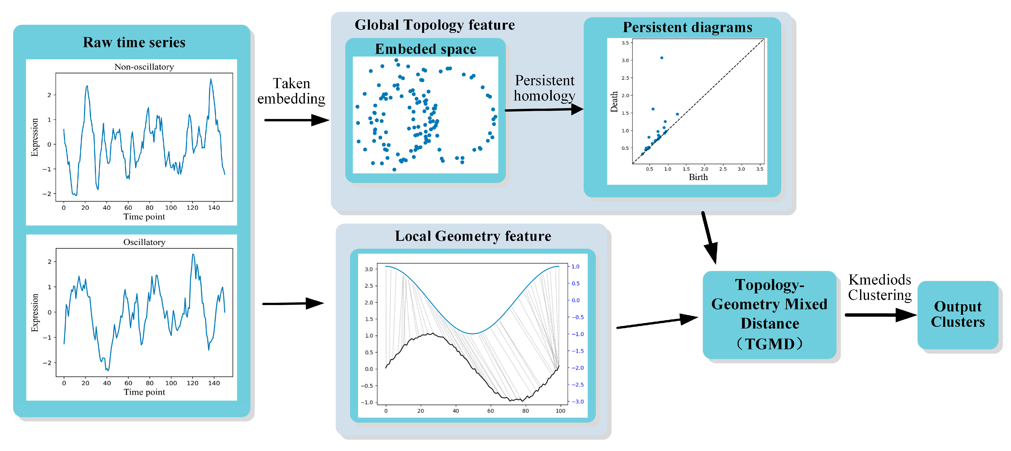
• We propose a TGMD measure for time series clustering analysis by combining the local geometric and global topological features of time series. Topology is a generic representation that enables a qualitative description of global features of a time series, while geometry describes local quantitative differences of the raw time series.
• Our mixed distance measure is based on a tuning function that modulates the TGMD matrix according to the proximity of topological properties.
• Experiments confirm that the method proposed in this paper outperforms topological-only methods or geometric-only methods in clustering noisy biological data for oscillatory activity clustering identification. Additionally, our method achieves competitive results on real datasets compared with other standard time series clustering methods. The visualization of TGMD metric space also demonstrate its effectiveness.

The rest of the paper is organized as follows. In Section 2, we review the main ideas about time series clustering together with the relevant literature. In Section 3, the proposed method is described in detail. The fourth Section is devoted to introducing the experimental setup and discussing results. Finally, Section 5 closes the paper with some concluding remarks about current results and future work.

2. Background and Previous Work

Time series clustering has been used for pattern recognition in different scientific fields because it enables data analysts to extract valuable information from complex and massive datasets.

2.1. Time Series Similarity Measures

The main idea of clustering is to group similar objects. Time-series clustering relies on distance measure to a high extent [1]. In order to discover which data are similar, different metrics may be applied to measure the distance between time series. One class of methods is based on quantifying local similarities directly on the raw time series, and the most commonly used metric is the Euclidean distance (ED), i.e., $d_{L_p}(\mathrm{X},\mathrm{Y})={({\sum }_{i=1}^t{\left(x_i-y_i\right)}^p)}^{\frac{1}{p}}$ with p = 2. ED has been widely used in time series clustering because it possesses a clear meaning and is easy to calculate [22]. However, it ignores the trend of the time series since the paired points between the two time series are fixed. To solve this problem, different approaches, e.g., DTW, have been put forward to measure the similarity between time series by stretching or contracting the time axis. DTW was introduced by Berndt and Clifford [23] to study similarities in speech recognition. Petitjean et al. [24] proposed a k-DBA algorithm based on DTW to improve alignment, which develops a global technique for averaging a set of sequences.

Shape-based distances are invariant with respect to scaling and shifting [25]. In order to reveal temporal dynamics, Yang et al. [26] developed a K-spectrum center-of-mass (K-SC) method that uses a similarity metric that is both shift-invariant and scale-invariant. Paparrizos et al. [25] proposed a method called k-shape, which uses normalized intercorrelation metrics in order to consider their shapes when comparing time series. However, since all the points are taken into consideration, the above methods are usually sensitive to outliers and noise.

2.2. Topological Time Series Analysis

In recent years, some researchers have applied topological data analysis methods to clustering of time series and their analysis [13,14,27,28,29].

Pereira [10] proposed a clustering method that considers topological features and applied it to both temporal and spatial data. Since traditional clustering techniques ignore topological information, they are not suitable for scale invariant spatial distribution with similarity in the temporal data. To describe the topological property, this method computes summary statistics from the persistence diagrams and then combines them with classical k-means clustering. Seversky [15] proposed a new dataset and framework in order to exploit TDA techniques in time series analysis. This framework is able to characterize the complex time-varying events and dynamics of time series data by describing the topological features of the data after delay embedding, with topological distances considered as a similarity metric. Kim et al. [30] proved that after applying principal component analysis (PCA) to the embedded time series in phase space, the bottleneck distance between the persistence diagram of the original point cloud and the PCA one is equal to 0.

The persistence diagram is the final output of TDA, which gives a brief description of the topological information. There are also other methods based on extracting features of persistence diagram, such as Betti sequences or persistence landscapes. Umeda [12] has proposed a volatile time series classification method based on extracting the structure of the attractor using TDA. This method was applied to a learning architecture, inspired by convolutional neural networks, to extract topological features such as the Betti sequence. Since those features represent a fundamental property of the time series, this approach works for both chaotic and non-chaotic series. Gidea et al. [31] used the distance between persistence landscapes to perform k-means clustering. Majumdar [14] proposed a new approach for financial time series clustering and classification that is based on TDA and persistence landscape. Chen [32] proposed a method to extract features and perform clustering of categorical time series using TDA. The method consists of performing Walsh–Fourier transforms (WFT) on the classified series, then extracting the first-order persistence landscape from the persistence diagram, and finally clustering using the Divide and Combine K-Means Clustering method. The first-order persistence landscape of WFT detects the strongest temporal patterns in the classified time series. Their method of extracting time series data features is applicable to categorical time series and cannot analyze a broader range of temporal data.

In contrast, our method is based on the distance metric between the persistence diagrams without manually extracting the features of the persistence diagram. Moreover, we consider both the topological features and the geometric property of time series.

3. Methods

A schematic diagram of the proposed Topological-Geometric Mixed Distance (TGMD) time series clustering method is shown in Figure 1. It includes three parts: detection of topological similarity, detection of geometric similarity, and mixed distance-based time series clustering.

3.1. Global and Local Features Extraction

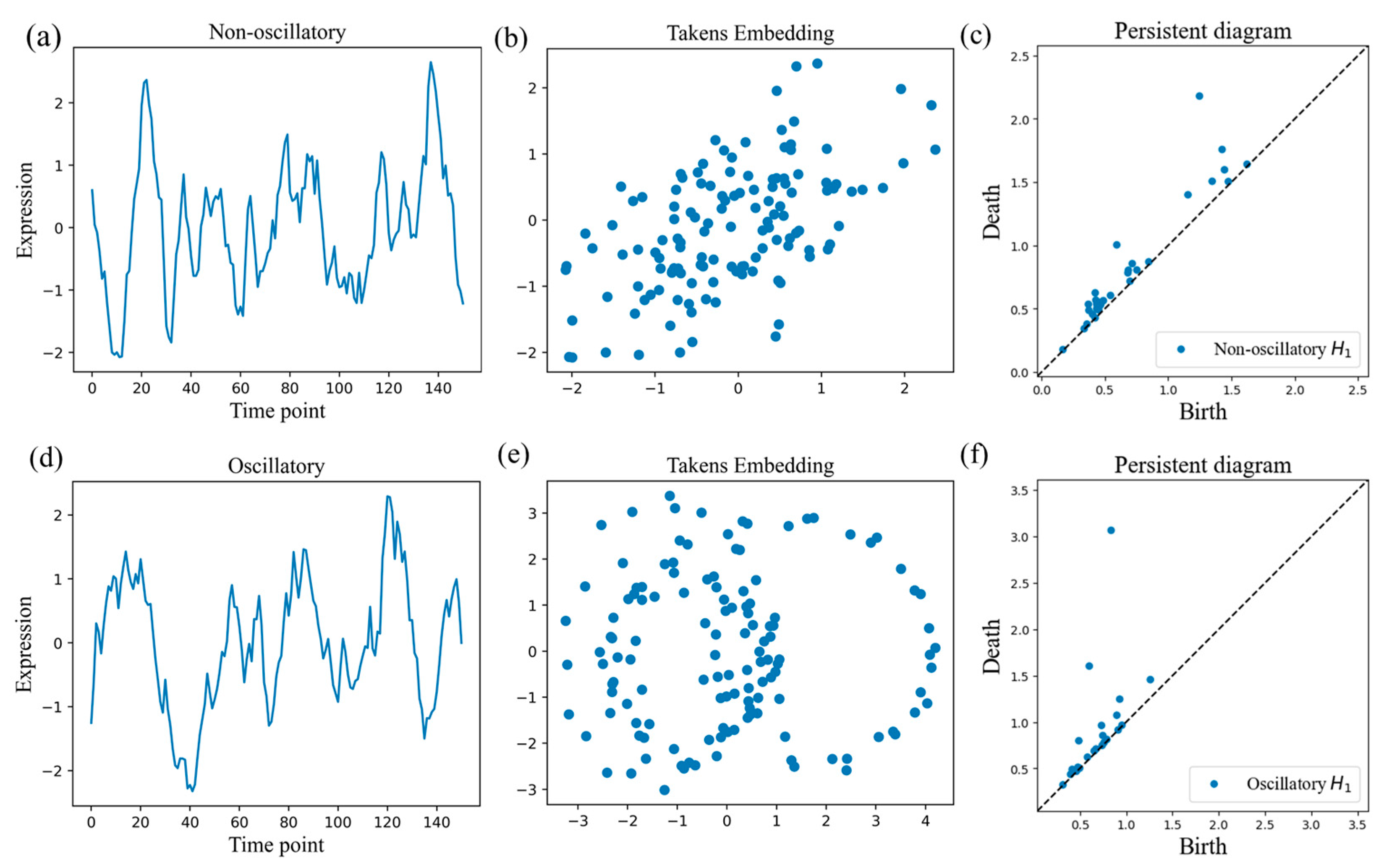
3.1.1. Global Topological Properties of Time Series

Let us consider a one-dimensional signal $f$ of length $T$, denoted by $\left\{x_t,t=1,2,\dots ,T\right\}$, i.e., a sequence of real numbers labeled by a time index, with $x_t$ representing the value at time $t$.

The unique topological features of a time series may be better appreciated in the phase space, which is obtained by time-delay embedding of the time series. A time series $f\left\{x_t,t=1,2,\dots ,T\right\}$ may be embedded into a cloud of points in the phase space $V_i=\left\{v_1,\dots ,v_t,\dots ,f_T\right\}$ [16], and these points are given by $v_i=\left(x_i,x_{i+\tau },\dots ,x_{i+\left(d-1\right)\tau }\right)$, where $d$ refers to the dimension of the embedded point cloud space, and $\tau$ denotes the delay factor. The number of points $N$ depends on the choice of $d$ and $\tau$, which, in turn, represent two relevant parameters. As a matter of fact, it is an inherently difficult problem to determine d and τ since real time series are noisy and have limited length. The optimal selection of τ depends on the objective of the analysis and is obtained by trial and error without using any systematic method [13]. In this paper, we consider $d$ and $\tau$ as hyperparameters and select them for clustering according to the silhouette coefficient [33].

$$S1\left(t\right)=sin\left(2\pi t\right)$$

(1)

$$S2\left(t\right)=sin\left(4\pi t\right)$$

(2)

$$S3\left(t\right)=sin\left(2\pi t\right)+\frac{1}{3}cos\left(4\pi t\right)$$

(3)

$$S4\left(t\right)=\frac{1}{3}sin\left(2\pi t\right)+cos\left(4\pi t\right)$$

(4)

In phase space, the relevant topological features of time series are mainly 0-dimensional components and 1-dimensional loops. Considering the examples shown in Figure 2, S1–S3 are all periodic time series, see Equations (1)–(3), whereas S4 is a non-periodic time series with Equation (4). S1–S3 all have similar topology in the embedding space, i.e., a one-dimensional ring structure, and we cannot distinguish them from each other or from their global topology. Meanwhile, S1 and S3 are closer to each other than S1 is to S2 by calculating their mutual DTW distances, which is due to local differences. Since the frequency of S2 is higher compared with S1 and S3, if we compare DTW distances we find that S1 and S4 are closer to each other than S1 is to S2. However, upon considering the topological properties of data, we will find that S1 and S2 are different from S4. Therefore, by considering different properties of time series, we may gain more information than focusing on either local or global ones.

After embedding the time series in phase space, we apply PCA to this embedded point cloud to reduce topological noise. Then we use persistent homology and persistence diagram as a description of its topological properties. Persistent homology describes the topological characteristics of the whole filtration process, which captures the growth, birth, and death of different topological features across dimensions (e.g., components, tunnels, voids). And the persistence diagram is a brief description of the topological changes of the data at different scales $\epsilon$.

We rely on the construction of the simple complex $K$ for persistent homology. A simplicial complex $K$ is a collection of finite sets such that $\sigma \in K$ and $\alpha \in \sigma$, then $\alpha \in K$. For every $\alpha \in \sigma \in K$, $\alpha$ is the face of $\sigma$, its coface. If $\sigma \in K$ has cardinality $\left|\sigma \right|=k+1$, we say $\sigma$ a k-simplex of dimension $k$, $dim\left(\sigma \right)=k$. A simplicial complex can be embedded in Euclidean space as the union of its geometrically realized simplices such that they only intersect along shared faces. The topological properties are described by topological features such as components, loops, and voids of different dimensions of the simple complex form ($H_0,H_1,H_2$, etc.). In the point cloud, we construct a complex on this set of points, where the pairwise distances of points satisfy $d\le 2\epsilon$, $\epsilon$ being a non-negative scale parameter, and different values of $\epsilon$ result in different complex and topological information. Let $\epsilon$ grow from 0: if ε is very small, then no links between points are created. As $\epsilon$ grows, there will be links between points to form a complex, with different topological information appearing. If $\epsilon$ continues to increase, links continue to exist, and if the value of $\epsilon$ exceeds a certain threshold, links are created between all points, and we cannot observe useful topological information. By considering a set of increasing value for $\epsilon$ (${\epsilon }_1<{\epsilon }_2<{\epsilon }_3<\dots <{\epsilon }_n$), we build a set of simplicial complexes, a process we call filtration (see an example in Figure 3). The Vietoris–Rips (VR) complex (or Rips complex) is commonly used to construct simple complexes, which are based on the pairwise distances between their vertices. Suppose we are given a finite set of n-dimensional points $S\subseteq R^n$, such as the example of set with 16 points in the plane in Figure 3. The VR complex $V_{\epsilon }\left(S\right)$ of $S$ at scale $\epsilon$ is

$$V_{\epsilon }\left(S\right)=\{\sigma \subseteq S|d\left(u,v\right)\le \epsilon , \forall u\ne v\in \sigma \}$$

(5)

where $d$ is the Euclidean distance metric. In other words, each simplex $\sigma$ in $V_{\epsilon }\left(S\right)$ has vertices that are pairwise within distance.

As shown in Figure 3g, each point $\left(b,d\right)$ in the persistence diagram represents the topological feature of a 1-dimensional hole (e.g., loops or tunnels are 1-dimensional holes) which appears at $\epsilon =b$ (stands for the birth scale) and disappears at $\epsilon =d$ (stands for the death scale). In fact, we are interested in how long a certain topological feature persists in the filtering, since a longer persistence (the difference between the death time and the birth time) indicates more robust topological features of data. On the contrary, a shorter persistence may be considered as topological noise. This information describes the topological features of the time series after embedding and provides valuable insights into the dynamics of the time series, for instance, the emergence of an oscillation in a time series can be attributed to the birth of a 1-dimension hole in the embedded space. Using these global features, the qualitative properties of the time series can be captured in a robust and effective way. For a more detailed description of topological data analysis with respect to persistent homology, see Edelsbrunner [17].

3.1.2. Local Properties of Time Series

Time series are uniquely represented by their geometric shape in the original space, which also carries information [34]. For example, seismometer signals (amplitude of time vs. surface rhythm) contain information about earthquakes, and the shape of financial time series may reveal the trend of the stock market, e.g., double tops/bottoms, head and shoulders, triangle, flag, and rounded top/bottom. In our methods, we can calculate the distance of local point pairs in the raw time series to capture these similarities in shape.

3.2. Topological-Geometric Mixed Distance

3.2.1. Topological Similarity

As mentioned above, we use a persistence diagram to describe the topological features of time series. One of the properties of a persistence diagram is stability, i.e., the fact that small perturbations of data have a minimal impact on the generation of the persistence diagrams [20]. This allows us to reliably quantify the differences in topological properties of time series by introducing a similarity measure between persistence diagrams. Persistence diagrams form a metric space under the Wasserstein metric [35]. The Wasserstein distance is the sum of p-th power of the distance between all points matching two persistence diagrams (see Figure 4). The p-th Wasserstein distance between two persistence diagrams $B$ and $B^{\prime }$ is defined as follows:

$$W_p\left(PD,P{D}^{\prime }\right)=\frac{inf}{\gamma :B\to B^{\prime }}{\left({{\displaystyle \sum }}_{u\in B}{\Vert u-\gamma \left(u\right)\Vert }_{\infty }^P)\right)}^{\frac{1}{p}}$$

(6)

where 1 ≪ $p<\infty$, $\gamma$ is the mapping between $PD$ and $P{D}^{\prime }$.

Meanwhile, Wasserstein distance is computationally complex. Based on Wasserstein distance, the Sliced Wasserstein distance [21] is an approximation of the Wasserstein distance. The Sliced Wasserstein distance is not only provably stable but also discriminative (its bounds depend on the number of points in the persistence diagrams). The basic idea of this metric is to slice the plane with lines through the origin, project the measurement onto these lines, where Wasserstein distance is computed, and integrate these distances over all possible lines. In this paper, we present clustering experiments using sliced Wasserstein distance as topological similarity measures.

3.2.2. Geometric Similarity of Time Series

The Euclidean distance and the DTW distance are the most popular geometric distances for time series. If $T_1=\left(u_1,\dots ,u_p\right)$ and $T_2=\left(v_1,\dots ,v_p\right)$ are two time series, the Euclidean distance ${\delta }_E$ between $T_1$ and $T_2$ is defined as:

$${\delta }_{ED}\left(T_1,T_2\right)={\left({\displaystyle \sum }_{i=1}^p{\left(u_i-v_i\right)}^2\right)}^{\frac{1}{2}}$$

(7)

whereas the DTW (dynamic time warping) is given by

$${\delta }_{DTW}\left(T_1,T_2\right)=\underset{r\in M}{min}\left|r\right|=\underset{r\in M}{min}\left({\displaystyle \sum }_{i=1,\dots ,m}\left|u_{ai}-v_{bi}\right|\right)$$

(8)

Geometric similarity measures tend to identify local geometric relationships and quantitative differences between two raw time series samples without considering the changes in the topological structure of time series. We therefore propose a new similarity metric that combines a topological similarity metric with a traditional similarity one.

3.2.3. Topological-Geometric Mixed Distance

The novel distance is built from using a tuning function, which is chosen to make the topological similarity ($TS$) an adjusting factor for TGMD. If the topological properties of the two time series are different, then the tuning function increases the TGMD measure, otherwise it decreases the TGMD measure. We choose an exponential form function instead of a linear form. Since the exponential form function gives a different increasing or decreasing speed around the extreme values (1 and 0), a nearly equal modulating effect for the extreme values and their nearest neighbors can be secured (see Figure 5).

To this aim, we first rescale the topological similarity ($TS$) to obtain a normalized topological similarity ($T{S}^{\prime }$) as follows:

$$T{S}^{\prime }\left(T_1,T_2\right)=\frac{TS\left(T_1,T_2\right)-T{S}_{min}}{T{S}_{max}-T{S}_{min}}$$

(9)

Then, a monotonically increasing tuning function $f\left(x\right)$ as follows:

$$f\left(x\right)=\frac{2}{1+e^{-k\left(2x-1\right)}}$$

(10)

where k is a positive adjustment factor, k ≥ 0, which is used to rescale the topological similarity metric.

Combining the above process, we propose the following similarity metric TGMD as follows:

$$TGMD\left(T_1,T_2\right)=f\left(T{S}^{\prime }\left(T_1,T_2\right)\right)\times Geo\left(T1,T2\right)$$

(11)

The tuning function adjusts the TGMD metric according to the similarity of the topologies. If the topological similarity ($TS$) of two time series is close to 1, for any $k\ge 0$, there is the tuning function $f\left(x\right)\ge 1$, which increases the TGMD metric. The scaling factor due to topological similarity increases with k.

3.2.4. Clustering Algorithms

The choice of clustering algorithm may depend on the strategy employed, i.e., maximizing intra-group similarity and minimizing inter-group similarity. The K-medoids algorithm optimizes clusters by minimizing the distance between the center of each cluster (i.e., the centroid) and the data points within that cluster, and finally generates spherical clusters of similar size. The centroid may or may not be an actual data point. K-medoids is one of the most popular partitional clustering algorithms in time series analysis [1]. In this article, we use the k-medoids algorithm for clustering analysis, together with the proposed TGMD similarity metric.

4. Experiment

4.1. Experiment Datasets

4.1.1. Synthetic Single-Cell Data

Based on the model of the Hes1 oscillator [36], we generated synthetic mRNA and protein time series data, which were modeled as a negative auto-regulatory system with delays [13]. This time series datasets were divided into two categories, including periodic and non-periodic ones. We simulated data from 200 cells of the Hes1 model in oscillatory and non-oscillatory regimes and measured protein levels every $v=5, 10, 15, 20$ min in the interval from 5000 min to 6500 min. After obtaining time series at different intervals, the data were normalized to have a mean value of 0 and unit variance, and the Gaussian noise was added.

4.1.2. UCR Time Series Archive

The UCR time series archive [37] is an important resource for the time series data-mining community, and we selected 11 typical datasets from UCR to evaluate the clustering performance of the proposed algorithm. These datasets contained data with different sizes, lengths, number of classes, and signal types. Details are summarized in

Table 1. The statistics of 11 datasets from the UCR Time Series Archive.

Dataset	Data Size	Length	No. of Classes	Type
Synthetic Control	600	60	6	SIMULATED
ECG200	200	96	2	ECG
ECGfiveday	884	136	2	ECG
ECG5000	500	140	5	ECG
TwoLeadECG	1162	82	2	ECG
Fish	350	463	7	IMAGE
Face four	112	350	4	IMAGE
DiatonSizeReduction	322	345	4	IMAGE
ItalyPowerDemand	1096	24	2	SENSOR
Trace	200	275	4	SENSOR
GunPoint	200	150	2	MOTION

.

4.2. Baselines and Metrics

4.2.1. Baselines

The proposed TGMD clustering method was compared with other clustering methods for time series data. In particular, we considered the commonly used distance metric ED and DTW as geometric methods and used k-mediods for clustering (k-med-ED and k-med-DTW). Then we considered the ED of the PCA subspace as a distance metric and used k-means for time series clustering. We also compared TGMD results with those coming from k-shape [25] and TSKMeans [38] (by using their implementation in Tslearn [39]). TSKMeans is a k-means type smooth subspace clustering algorithm which may effectively exploit subspace information inherently contained in the time series datasets to improve the clustering performance.

4.2.2. Metrics

Typically, clustering consists of exploring data without true labels. In this paper, we used the following metrics to measure the effectiveness of the method.

Silhouette Coefficient [33]. If the ground truth label is unknown, the model itself must be used for evaluation. Higher silhouette coefficient scores are associated with models having better defined clusters. A silhouette coefficient is defined for each sample, which consists of two scores. The silhouette coefficient $s$ for a single sample is calculated as:

$$s=\frac{b-a}{\max \left(a,b\right)}$$

(12)

where $a$ is the average distance between the sample and all other points in the same category, and $b$ is the average distance between the sample and all other points in the second closest cluster.

Adjusted Rand index (ARI) [40]. ARI has been introduced to address the Rand index (RI) issues in describing the similarities among the random assignment cluster class marker vectors. ARI measures the similarity of two assignments without considering alignment and chance normalization. The value of the ARI is in the range (−1,1), where a negative value indicates bad clustering and 1 means perfectly correct clustering. For two random divisions, the ARI is a constant close to 0. RI and ARI are calculated as:

$$RI=\frac{TP+TN}{TP+TN+FP+FN}$$

(13)

$$ARI=\frac{RI-E\left[RI\right]}{max\left(RI\right)-E\left[RI\right]}$$

(14)

where $TP$ is the number of time series pairs belonging to the same category and assigned to the same cluster, $TN$ is the number of time series pairs belonging to different categories and assigned to different clusters, $FP$ is the number of time series belonging to different categories but assigned to the same cluster, and $FN$ is the number of time series pairs belonging to the same category but assigned to different clusters.

4.3. Experimental Setup

At first, we tested the performance of three different distance measures on synthetic single-cell data: DTW (geometric-only), Sliced Wasserstein (topological-only), and TGMD, clustering them using k-mediods. We analyzed the clustering results using ARI and compared performance for different dimension $d$, where $d\in \left\{2,3,4,5,6,7,8,9,10\right\}$.

In the second stage, we tested the clustering performance of the proposed algorithm on real datasets and compared results with those of the other methods mentioned in Section 4.2.1. In our method, we hand-selected the delay embedding parameters $\tau$ and $d$ according to the silhouette coefficient on different datasets. For the tuning function, we chose $k=1$, and used Euclidean and DTW distances to assess geometric similarity.

Finally, we visualized TGMD metric space on the Synthetic Controls dataset by Uniform Manifold Approximation and Projection (UMAP) [41]. UMAP is a dimension reduction algorithm that proposed to model and preserve the high-dimensional topology of data points in the low-dimensional space. Empirically, we set $d=15$ and $\tau =3$ to implement delayed embedding and compared the effects of different adjustment factors k on the results.

4.4. Clustering Analysis of the Synthetic Single-Cell Data

In this Section, we analyze the results of clustering on synthetic single-cell data. Figure 6a,d shows examples of non-oscillatory and oscillatory time series data, respectively, taken every 5 min. Figure 6b,e shows the two time series in the phase space. For the oscillatory time series, Figure 6e reveals a clear topological signal (a loop), compared with the results of Figure 6b, where no topological feature appears. We then use persistent homology to obtain topological features: Figure 6c,f shows the persistence diagrams that represent a topological summary of the point cloud in the phase space. In Figure 6c, most of the points are close to the diagonal, which may be interpreted as topological noise. In Figure 6f, instead, we clearly see the presence of a point far away from the diagonal, i.e., a persistent topological signal. In this example, it is clear how to distinguish non-oscillatory data from oscillatory data by persistence diagrams.

Next, we performed clustering analysis of synthetic single-cell data using TGMD and compared the effect of different embedding dimension $m$. We used both silhouettes coefficient and ARI as evaluation metrics. As shown in Figure 7, the qualitative behavior of silhouettes and ARI as a function of m was similar, and their minima and maxima coincided. We notice that since the length of the time series became shorter for increasing $v$, clustering became increasingly difficult. As a consequence, as $v$ increased, better clustering performance was obtained for larger m, since higher dimensional information was needed to properly describe data.

To demonstrate that TGMD is more robust than the topological-only (TS) or geometry-only (DTW) methods when time series are being perturbed by noise, we compared the performance of these methods on noisy time series data. We added Gaussian noise with different magnitudes ${\sigma }_n^2=0.1, 0.3, 0.5, 0.7$ at measurement intervals of $\nu =10$ min. Figure 8 depicts the average clustering result and shows that TGMD outperformed topological-only or geometry-only methods in the entire range of ${\sigma }_n^2$, from $0.1$ to $0.7$.

4.5. Clustering Analysis of the Real Time Series Data

In order to further assess performance of the TGMD method (k-med-TGMD) in classifying different real dataset, we considered different embedding dimensions $d=2,3,\dots , 20$, and different delays $\tau =1,2,3,4$ and sought the optimal values. In doing this, we assumed $k=1$ for the adjustment parameter of the tuning function and used Euclidean or DTW distance to capture geometric properties of the raw time series. Further, we compared the proposed method with other clustering methods for time series data. The results of the test are shown in

Table 2. Clustering results for 11 datasets taken from UCR Time Series Archive. TGMD is the method proposed in this paper. The best and second-best methods in terms of accuracy for each dataset are highlighted in red and yellow, respectively.

Datasets	TS Kmeans	PCA-Kmeans	Kshape	k-med-DTW	k-med-ED	k-med-TGMD (DTW + TS)	k-med-TGMD (ED + TS)
Synthetic Controls	0.5902	0.6157	0.6080	0.6502	0.3765	0.8238	0.5048
ECG200	0.0783	0.2194	0.1802	0.0981	0.2640	0.3096	0.3135
ECGfiveday	−0.0275	−0.0434	0.6680	0.0515	0.0042	0.3993	0.2398
Two lead ECG	0.1136	0.0535	0.0502	−0.0254	0.1129	0.2877	0.1129
ECG5000	0.4253	0.4849	0.3859	0.4014	0.4943	0.4448	0.5726
Face four	0.3464	0.3377	0.3833	0.3548	0.2376	0.7283	0.2844
fish	0.3653	0.1796	0.1515	0.2061	0.1801	0.3230	0.2362
Italy power	0.0025	0.0025	0.5277	0.4427	0.8263	0.4843	0.8263
Trace	0.6160	0.3266	0.3319	0.6288	0.3649	0.6810	0.6730
GunPoint	0.1148	−0.0053	−0.0053	−0.0050	−0.0050	0.2775	0.2470
DiatomSizeReduction	0.8607	0.5221	0.4348	0.6450	0.6669	0.7857	0.8267

below, where the best and second-best method (in terms of accuracy) are highlighted in red and orange, respectively. The results in Table 2 show that the TGMD provided better results than methods that considered only the geometric properties of the original time series (DTW and ED). For the 11 datasets considered here, our method was the best one in eight cases and the second best in three cases.

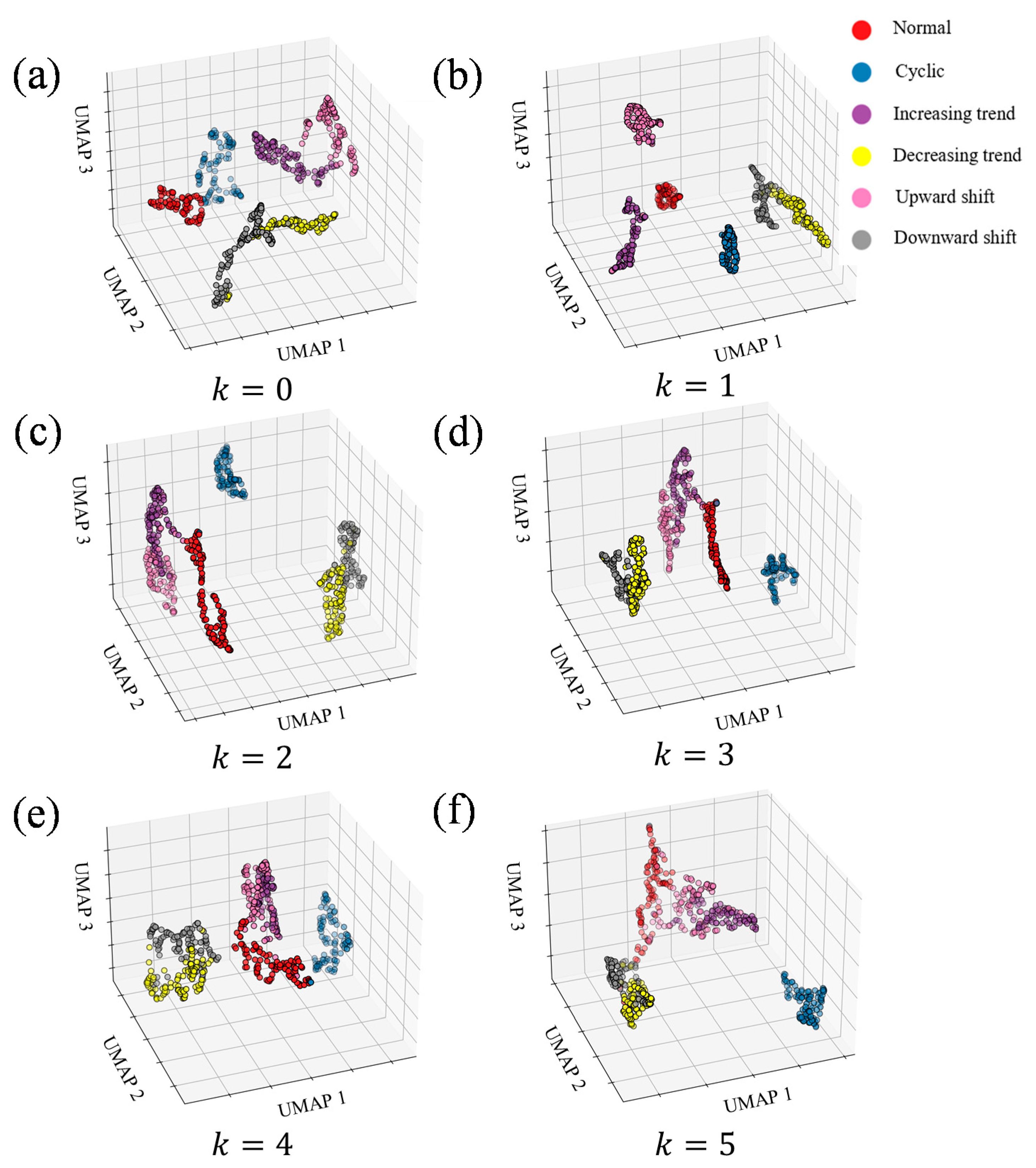
4.6. Visualization Analysis

In this Section, we analyze the effect of the adjustment parameter k on the clustering performance of TGMD on the Synthetic Controls dataset. Then, we visualize the TGMD metric space using UMAP [41].

The Synthetic Controls dataset was used to monitor the behavior of the system, with 600 data and a timing length of 60. There were six types of patterns within this dataset: normal, periodic, downward movement, upward movement, upward trend, and downward trend, respectively. All patterns except the normal pattern indicated that the monitored process was not functioning properly and needed to be adjusted.

When $k=0$, $f\left(x\right)$ was constant (see Figure 5), TGMD just reflected the geometric properties of the original time series (Figure 9a). Therefore, the two types of increasing trend (purple) and upward shift (pink) with different temporal dynamics were not easily distinguished. As $k$ increased, TGMD started to reveal the topological properties of the time series. As is apparent from Figure 9b, TGMD distinguished between increasing trend (purple) and upward shift (pink) already for $k=1$. As $k$ increased, only cycles with distinct topological properties were clearly distinguished (see results for $k=5$). Furthermore, we performed a cluster analysis on the distance matrix applied to the median value of $k$ and evaluated the result by ARI (Figure 10), which was similar to the visualization result. Overall, these results confirm that we may better understand the intrinsic properties of temporal data by properly considering the topological and geometric properties of the time series.

5. Conclusions

In this paper, a TGMD time series clustering framework was proposed and analyzed in detail. Using delay embedding, raw time series were projected in the phase space and then the topological features of the resulting point cloud were extracted using persistent homologies. A mixed distance measure based on a tuning function was suggested, which not only considers global topological properties but also describes the local structures of the time series. TGMD achieves this goal by taking into account the topological similarities, as well as the geometric ones. We performed a set of experiments, which showed that the method proposed in this paper outperforms topological-only or geometric-only methods in clustering noisy biological data. The proposed method achieves promising results compared with other standard time series clustering methods on real datasets, and the visualization analysis also verifies its effectiveness. These results show that consideration of both geometric and topological features can be used to reveal the representative features of an original time series to help time series clustering analysis.

Since the geometric and topological properties of a time series reveal its intrinsic characteristics, the proposed framework may be useful for clustering temporal data in different fields. Furthermore, the extraction of topological features from time series requires the use of delay embedding. This is the limitation of using topological features in time-series data analysis. Currently, the method takes into account only the topological properties in $H1$ dimension. In the future we intend to explore higher dimensional topological information since they are likely to reveal more complex topological properties that are potentially useful for improving clustering.

References

1. Aghabozorgi, S.; Shirkhorshidi, A.S.; Wah, T.Y. Time-series clustering—A decade review. Inf. Syst. 2015, 53, 16–38. [Google Scholar] [CrossRef]
2. Subhani, N.; Rueda, L.; Ngom, A.; Burden, C.J. Multiple gene expression profile alignment for microarray time-series data clustering. Bioinformatics 2010, 26, 2281–2288. [Google Scholar] [CrossRef] [Green Version]
3. Liu, X.; Tian, Y.; Zhang, X.; Wan, Z. Identification of Urban Functional Regions in Chengdu Based on Taxi Trajectory Time Series Data. ISPRS Int. J. Geo-Inf. 2020, 9, 158. [Google Scholar] [CrossRef] [Green Version]
4. Gajowniczek, K.; Bator, M.; Ząbkowski, T. Whole Time Series Data Streams Clustering: Dynamic Profiling of the Electricity Consumption. Entropy 2020, 22, 1414. [Google Scholar] [CrossRef]
5. Hsu, Y.-C.; Chen, A.-P. A clustering time series model for the optimal hedge ratio decision making. Neurocomputing 2014, 138, 358–370. [Google Scholar] [CrossRef]
6. Chu, S. Iterative deepening dynamic time warping for time series. In Proceedings of the 2002 SIAM International Conference on Data Mining. Society for Industrial and Applied Mathematics, Arlington, VA, USA, 11–13 April 2002; pp. 148–156. [Google Scholar]
7. Faloutsos, C.; Ranganathan, M.; Manolopoulos, Y. Fast subsequence matching in time-series databases. ACM Sigmod Rec. 1994, 23, 419–429. [Google Scholar] [CrossRef] [Green Version]
8. Vlachos, M.; Kollios, G.; Gunopulos, D. Discovering similar multidimensional trajectories. In Proceedings of the 18th International Conference on Data Engineering, San Jose, CA, USA, 26 February–1 March 2002; pp. 673–684. [Google Scholar]
9. Li, Y.; Liu, R.W.; Liu, Z.; Liu, J. Similarity Grouping-Guided Neural Network Modeling for Maritime Time Series Prediction. IEEE Access 2019, 7, 72647–72659. [Google Scholar] [CrossRef]
10. Pereira, C.M.M.; de Mello, R.F. Persistent homology for time series and spatial data clustering. Expert Syst. Appl. 2015, 42, 6026–6038. [Google Scholar] [CrossRef]
11. Ferreira, L.N.; Zhao, L. Time series clustering via community detection in networks. Inf. Sci. 2016, 326, 227–242. [Google Scholar] [CrossRef] [Green Version]
12. Umeda, Y. Time Series Classification via Topological Data Analysis. Inf. Media Technol. 2017, 12, 228–239. [Google Scholar] [CrossRef] [Green Version]
13. Tran, Q.H.; Hasegawa, Y. Topological time-series analysis with delay-variant embedding. Phys. Rev. E 2019, 99, 032209. [Google Scholar] [CrossRef] [Green Version]
14. Majumdar, S.; Laha, A.K. Clustering and classification of time series using topological data analysis with applications to finance. Expert Syst. Appl. 2020, 162, 113868. [Google Scholar] [CrossRef]
15. Seversky, L.M.; Davis, S.; Berger, M. On Time-Series Topological Data Analysis: New Data and Opportunities. In Proceedings of the 2016 IEEE Conference on Computer Vision and Pattern Recognition Workshops (CVPRW), Las Vegas, NV, USA, 26 June–1 July 2016; pp. 1014–1022. [Google Scholar]
16. Takens, F. Detecting strange attractors in turbulence. In Dynamical Systems and Turbulence, Warwick 1980; Springer: Berlin/Heidelberg, Germany, 1981; pp. 366–381. [Google Scholar]
17. Edelsbrunner, H.; Letscher, D.; Zomorodian, A. Topological persistence and simplification. In Proceedings of the 41st Annual Symposium on Foundations of Computer Science, Redondo Beach, CA, USA, 12–14 November 2000; pp. 454–463. [Google Scholar]
18. Zomorodian, A.J. Topology for Computing; Cambridge University Press: Cambridge, UK, 2005; Volume 16. [Google Scholar]
19. Carlsson, G. Topology and data. Bull. Am. Math. Soc. 2009, 46, 255–308. [Google Scholar] [CrossRef] [Green Version]
20. Cohen-Steiner, D.; Edelsbrunner, H.; Harer, J. Stability of Persistence Diagrams. Discret. Comput. Geom. 2007, 37, 103–120. [Google Scholar] [CrossRef] [Green Version]
21. Carrière, M.; Cuturi, M.; Oudot, S. Sliced Wasserstein Kernel for Persistence Diagrams. In Proceedings of the 34th International Conference on Machine Learning, Proceedings of Machine Learning Research, Sydney, Australia, 6–11 August 2017; pp. 664–673. [Google Scholar]
22. Yin, J.; Wang, R.; Zheng, H.; Yang, Y.; Li, Y.; Xu, M. A new time series similarity measurement method based on the morphological pattern and symbolic aggregate approximation. IEEE Access 2019, 7, 109751–109762. [Google Scholar] [CrossRef]
23. Berndt, D.J.; Clifford, J. Using dynamic time warping to find patterns in time series. In Proceedings of the KDD Workshop, Seattle, WA, USA, 31 July 1994; pp. 359–370. [Google Scholar]
24. Petitjean, F.; Ketterlin, A.; Gançarski, P. A global averaging method for dynamic time warping, with applications to clustering. Pattern Recognit. 2011, 44, 678–693. [Google Scholar] [CrossRef]
25. Paparrizos, J.; Gravano, L. k-shape: Efficient and accurate clustering of time series. In Proceedings of the 2015 ACM SIGMOD International Conference on Management of Data, New York, NY, USA, 31 May–4 June 2015; pp. 1855–1870. [Google Scholar]
26. Yang, J.; Leskovec, J. Patterns of temporal variation in online media. In Proceedings of the fourth ACM International Conference on Web Search and Data Mining, Hong Kong, China, 9–12 February 2011; pp. 177–186. [Google Scholar]
27. Zulkepli, N.F.S.; Noorani, M.S.M.; Razak, F.A.; Ismail, M.; Alias, M.A. Cluster Analysis of Haze Episodes Based on Topological Features. Sustainability 2020, 12, 3985. [Google Scholar] [CrossRef]
28. Perea, J.A. SW1PerS: Sliding windows and 1-persistence scoring; discovering periodicity in gene expression time series data. BMC Bioinform. 2015, 16, 1–12. [Google Scholar] [CrossRef] [PubMed] [Green Version]
29. Frahi, T.; Chinesta, F.; Falcó, A.; Badias, A.; Cueto, E.; Choi, H.Y.; Han, M.; Duval, J.-L. Empowering Advanced Driver-Assistance Systems from Topological Data Analysis. Mathematics 2021, 9, 634. [Google Scholar] [CrossRef]
30. Kim, K.; Kim, J.; Rinaldo, A. Time series featurization via topological data analysis. arXiv 2018, arXiv:1812.02987. [Google Scholar]
31. Gidea, M.; Goldsmith, D.; Katz, Y.; Roldan, P.; Shmalo, Y. Topological recognition of critical transitions in time series of cryptocurrencies. Phys. A Stat. Mech. Appl. 2020, 548, 123843. [Google Scholar] [CrossRef] [Green Version]
32. Chen, R.; Zhang, J.; Ravishanker, N.; Konduri, K.J. Clustering Activity–Travel Behavior Time Series using Topological Data Analysis. J. Big Data Anal. Transp. 2019, 1, 109–121. [Google Scholar] [CrossRef] [Green Version]
33. Rousseeuw, P.J. Silhouettes: A graphical aid to the interpretation and validation of cluster analysis. J. Comput. Appl. Math. 1987, 20, 53–65. [Google Scholar] [CrossRef] [Green Version]
34. Majumdar, K.; Jayachandran, S. A geometric analysis of time series leading to information encoding and a new entropy measure. J. Comput. Appl. Math. 2018, 328, 469–484. [Google Scholar] [CrossRef] [Green Version]
35. Mileyko, Y.; Mukherjee, S.; Harer, J. Probability measures on the space of persistence diagrams. Inverse Probl. 2011, 27, 124007. [Google Scholar] [CrossRef] [Green Version]
36. Monk, N.A.M. Oscillatory Expression of Hes1, p53, and NF-κB Driven by Transcriptional Time Delays. Curr. Biol. 2003, 13, 1409–1413. [Google Scholar] [CrossRef] [Green Version]
37. Dau, H.A.; Bagnall, A.; Kamgar, K.; Yeh, C.M.; Zhu, Y.; Gharghabi, S.; Ratanamahatana, C.A.; Keogh, E. The UCR time series archive. IEEE/CAA J. Autom. Sin. 2019, 6, 1293–1305. [Google Scholar] [CrossRef]
38. Huang, X.; Ye, Y.; Xiong, L.; Lau, R.Y.K.; Jiang, N.; Wang, S. Time series k-means: A new k-means type smooth subspace clustering for time series data. Inf. Sci. 2016, 367–368, 1–13. [Google Scholar] [CrossRef]
39. Tavenard, R.; Faouzi, J.; Vandewiele, G.; Divo, F.; Androz, G.; Holtz, C.; Payne, M.; Yurchak, R.; Rußwurm, M.; Kolar, K. Tslearn, a machine learning toolkit for time series data. J. Mach. Learn. Res. 2020, 21, 1–6. [Google Scholar]
40. Hubert, L.; Arabie, P. Comparing partitions. J. Classif. 1985, 2, 193–218. [Google Scholar] [CrossRef]
41. McInnes, L.; Healy, J.; Melville, J. Umap: Uniform manifold approximation and projection for dimension reduction. arXiv 2018, arXiv:1802.03426. [Google Scholar]
Figure 1. Schematic diagram of the proposed time series clustering method with Topological-Geometric Mixed Distance.
Mathematics 09 01046 g001
Figure 2. (ad) Time series S1–S4 in the original space; (eh) Time series S1–S4 in the phase space.
Mathematics 09 01046 g002
Figure 3. An example of VR complexes with resulting persistence diagram. We consider the 1-dimension hole ( H 1 ) here. From (af), we let the radius ε grow gradually. As ε increases, a 1-dimension hole appears and disappears in the region. The first 1-dimensional hole (yellow loop) appears at (c), and the second (red loop) appears at (d). If we continue increasing ε , then the yellow loop disappears at (e), and the red loop disappears at (f). (g) Persistence diagram corresponding to topological changes in the previous VR complex. There are two persistence points ( 0.28 ,   0.48 ) and ( 0.37 ,   0.82 ) , which represent the birth and death of the yellow loop and the red loop, respectively. A persistence diagram is a collection of all persistence points in the filtration.
Mathematics 09 01046 g003
Figure 4. The Wasserstein distance is computed by matching all points. If no corresponding matching point is found, it will match to diagonal.
Mathematics 09 01046 g004
Figure 5. The adaptive tuning effect f(x).
Mathematics 09 01046 g005
Figure 6. (a,d) are two examples of non-oscillatory (a) and oscillatory (d) time series data generated by the Hes1 model. (b,e) are the visualization results of the time series data after delay embedding and projected to a two-dimensional plot by PCA. (c,f) are the corresponding one-dimensional persistence diagrams. (c) corresponds to the non-oscillatory data of (a). And (f) corresponds to the oscillatory time-series in (d).
Mathematics 09 01046 g006
Figure 7. Clustering results for synthetic single-cell data with different intervals. (ad): the results with v = 5 ,   10 ,   15 ,   20 . Clustering results are evaluated by ARI (yellow) and silhouette coefficient (blue).
Mathematics 09 01046 g007
Figure 8. Clustering results for synthetic single-cell data with different noises.
Mathematics 09 01046 g008
Figure 9. The TGMD metric space with different adjustment parameter visualized using UMAP. (af): the results with k = 1 ,   2 ,   3 ,   4 ,   5 , different colors represent different labels of the data.
Mathematics 09 01046 g009
Figure 10. Clustering results by different adjustment parameter k.
Mathematics 09 01046 g010