Overlap Detection in 2D Amorphous Shapes for Paper Optimization in Digital Printing Presses

Abstract

Paper waste in the mockups design with regular, irregular, and amorphous patterns is a critical problem in digital printing presses. Paper waste reduction directly impacts production costs, generating business and environmental benefits. This problem can be mapped to the two-dimensional irregular bin-packing problem. In this paper, an iterated local search algorithm using a novel neighborhood structure to detect overlaps between amorphous shapes is introduced. This algorithm is used to solve the paper waste problem, modeled as one 2D irregular bin-packing problem. The experimental results show that this approach works efficiently and effectively to detect and correct the overlaps between regular, irregular, and amorphous figures.

1. Introduction

The two-dimensional (2D) bin-packing problem (BPP) is a combinatorial optimization problem classified as NP-Complete [1] since no exact algorithm for this problem is known to run in polynomial time. Then, computational heuristics have to be used to find near-optimal problem solutions. 2D BPP consists of placing a set of usually small elements (pieces) in one or more large objects (bins) and optimizing some objective function. In digital printing presses, a bin is a paper sheet where elements (regular, irregular, or amorphous shapes) are placed without overlapping so that the residual area is minimal. The residual area is the difference between the paper sheet area and the sum of each of the shapes’ areas placed in it. It is then a geometric problem of optimally accommodating the shapes (regular, irregular, and amorphous) without overlapping them.

In the existing literature, there are several approaches to 2D irregular BPP. In [2], a Constructive Algorithm (CA) to the nesting problem with irregular pieces is introduced. The solution is built by successively adding a new one to a set of pieces previously placed on a plate. Several criteria to choose the next piece to be added and to define its orientation are also proposed. A not-fit polygon (NFP) algorithm to determine the feasible location points in the placed pieces’ contour is used. In [3], a tutorial of the primary geometric methodologies currently used for cutting and packaging irregular pieces is provided. They use the NFP algorithm as their insertion procedure. This algorithm traverses the inserted pieces’ contour, trying to place a new one as close as possible to this contour, considering its concavities. In [4], authors explore different problem representations and mechanisms to move between solutions and evaluate basic approaches to solve them. In [5], one ordered list of pieces to be packed represents the 2D irregular BPP, which is solved using both TOPOS and beam-search approaches. In [6], the 2D irregular (convex) BPP with guillotine constraints is solved using three two-stage strategies. These strategies first place one or two pieces in a rectangle area that is then packed using a competitive algorithm.

In [7], a one-dimensional (1D) BPP heuristic is adapted to solve the 2D irregular BPP. The authors carried out several tests using a wide variety of convex polygons and applied various insertion techniques, such as First Fit (FF), First Fit Decreasing (FFD), First Fit Increasing (FFI), Filler, and Best Fit (BF). Unlike the NFP method, these strategies insert polygons, omitting their concavities. The insertion is carried out by ordering the polygons and placing them, starting in the coordinates (0,0). In [8], several variants of a constructive algorithm able to solve a wide variety of 2D irregular BPP variants are described. This algorithm first applies an Integer Programming model to assign pieces to bins and then uses a Mixed Integer Programming model for placing the pieces into the bins. The second stage tests a promising set of rotations for the piece and puts the one that fits the piece into the bin. A tested method is the FF algorithm, which is similar to the FFD method proposed in [9] to solve the 1D BPP. FFD takes an ordered list of pieces and assigns them sequentially to bins. To assign a piece, FFD examines the bins in the order they are opened and places the piece in the first bin that it will fit into. If the piece does not fit in any existing bin, a new one is created, and the piece is assigned to it. This algorithm is efficient but critically dependent on the initial order of the pieces. In [10], an evolutionary hyper-heuristic that chooses the best of six deterministic algorithms to solve BPP instances, either 1D or 2D, and uses regular or irregular pieces is introduced. In [11], the Heuristic Search Diversification Mechanism (HSDM), addressing both the piece allocation and placement problems together, is proposed. The authors implemented several strategies to handle piece rotations, such as Bottom-Left, Minimum-Length, and Maximum Utilization. These strategies can use a set of four angles or unrestricted rotations. In [12], a review about mathematical models for the cutting and packing problem using 2D/3D construction techniques is detailed. Furthermore, authors use the technique to insert each piece at the bottom left of another already inserted. This technique considers the pieces already inserted to avoid overlapping between them and to be able to fill the spaces that were left empty in previous insertion stages. Finally, in [13], one improved typology of cutting and packing problems is introduced, based on the one proposed by Dyckhoff [14], but with a new criterion and setting new and different categories. The authors demonstrated the typology viability, classifying the papers in the existing literature between 1995 and 2004.

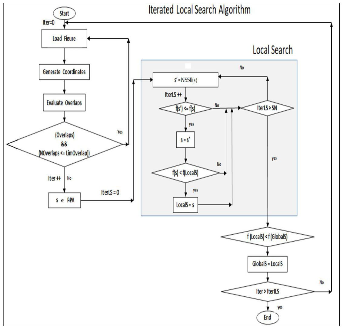
Unlike the approaches proposed in the existing literature, this article presents an iterated local search-based approach to insert pieces in bins. The iterated local search (ILS) is a powerful technique, simple to implement, robust, and highly efficient to traverse a complex solution space and reach near-optimal solutions [15,16]. In particular, in this paper, ILS uses a neighborhood structure that consists of making small movements on pieces previously placed in the bin to obtain more available space for new pieces. This neighborhood structure has been successfully used to solve various NP-complete problems [1]. For the paper waste reduction problem, the neighborhood structure is determined using a geometry-based method for overlap detection between pieces (regular, irregular, amorphous, or a combination of them) [4] and achieving feasible and optimized results. The experimental results show that this approach works efficiently and effectively to detect and correct the overlaps between regular, irregular, and amorphous figures.

The rest of this paper is organized as follows. Section 2 describes the paper waste reduction problem using a graphical representation and mathematical model based on the 2D BPP. The neighborhood structure proposed in this paper, as well as the ILS algorithm to solve the problem, is detailed in Section 3. Section 4 presents the experimental results obtained by the proposed method, and the comparison with those of several algorithms in the existing literature using five benchmark problems. Finally, the conclusions of this work are discussed in Section 5.

2. Paper Waste Reduction Problem in Digital Printing Presses

2.1. Graphical Representation

Figure 1 is a graphical representation of the mockup design for a possible serial production on one paper sheet’s printable area (PPA) using a digital press. The paper in the figure has a rectangular PPA (colored black) with several pieces of various sizes distributed in it. The minimization of the residual area is required, inserting as many pieces as possible in the PPA. The residual area is the difference between the PPA and the total area of the pieces.

2.2. Mathematical Model

The paper optimization problem in digital printing presses consists of placing as many pieces as possible in a rectangular region without overlap between them. The pieces should be placed inside the rectangular region known as the Printable Paper Sheet Area (PPA). The pieces arranged on a PPA are regular, irregular, amorphous pieces, or a combination of them. The mathematical model used in this work to solve the waste reduction problem in digital presses is based on that used to represent a 2D BPP in [17] and is an approximate model to solve the paper optimization problem in digital presses.

$$minf\left(W,H,w,h,a\right)=\left(W\ast H\right)-\sum \left(w_i\ast h_i\right)+\sum \left(w_i\ast h_i-a_i\right)$$

(1)

s.t.

$$0\le x_i\le W-w_i\hspace{1em}\hspace{1em}\hspace{1em}\hspace{1em}\hspace{1em}\hspace{1em}\hspace{1em}\hspace{1em}\hspace{1em}\hspace{1em}\forall i\in N$$

(2)

$$0\le y_i\le H-h_i\hspace{1em}\hspace{1em}\hspace{1em}\hspace{1em}\hspace{1em}\hspace{1em}\hspace{1em}\hspace{1em}\hspace{1em}\hspace{1em}\forall i\in N$$

(3)

$$x_i+w_i\le x_j\hspace{1em}\hspace{1em}\hspace{1em}\hspace{1em}\hspace{1em}\hspace{1em}\hspace{1em}\hspace{1em}\hspace{1em}\hspace{1em}\forall i,j\in N$$

(4)

$$x_j+w_j\le x_i\hspace{1em}\hspace{1em}\hspace{1em}\hspace{1em}\hspace{1em}\hspace{1em}\hspace{1em}\hspace{1em}\hspace{1em}\hspace{1em}\forall i,j\in N$$

(5)

$$y_i+h_i\le y_j\hspace{1em}\hspace{1em}\hspace{1em}\hspace{1em}\hspace{1em}\hspace{1em}\hspace{1em}\hspace{1em}\hspace{1em}\hspace{1em}\forall i,j\in N$$

(6)

$$y_j+h_j\le y_i\hspace{1em}\hspace{1em}\hspace{1em}\hspace{1em}\hspace{1em}\hspace{1em}\hspace{1em}\hspace{1em}\hspace{1em}\hspace{1em}\forall i,j\in N$$

(7)

$$x_i,y_i,w_{i,}{h}_i,W,H\in N$$

(8)

The objective Function (1) is to minimize the PPA residual area. W and H represent the PPA width and height, respectively. Vectors w and h are the dimensions of the regular polygons enveloping the amorphous pieces. $\sum \left(w_i\ast h_i-a_i\right)$ is the total residual area between regular polygons and amorphous pieces, and x_i and y_i are the coordinates of the upper left edge of the i-th piece inserted into the PPA. The PPA residual area is computed as follows: First, each i-th amorphous piece $a_i$ inside a regular polygon is encoded in a binary matrix $\left(w_i\ast h_i\right)$. In this matrix, values of 1 represent the piece pixels $a_i$, and values of 0 describe the rest of the polygon pixels $\left(w_i\ast h_i-a_i\right)$. Then, in Equation (1), the PPA residual area is the difference between the PPA $\left(W\ast H\right)$and the area used by all regular polygons, $\sum \left(w_i\ast h_i\right),$added to the rest of the polygon pixels, $\sum \left(w_i\ast h_i-a_i\right),$that is, the number of values of 0 in the encoded matrices.

Constraints in (2) and (3) indicate that each i-th piece must be within the PPA. Constraints (4)–(7) indicate that each i-th piece must not have an overlap, that is, each inequality means one of four relative locations: to the left of, to the right of, below, or above. Finally, according to (8), the mathematical model does not accept negative values in the variables.

The optimization model described in (1)–(8) represents the 2D BPP with a single bin. Since only one bin is used (a paper sheet’s printable area), it can be solved in polynomial time despite being an NP-complete problem [1]. This is an integer linear programming model that can be solved with commercial software such as CPLEX. CPLEX must be adapted to treating amorphous pieces, combining with the algorithms presented in this work to read pixel-based images and with overlap detection.

3. Neighborhood Structure

A solution s for the waste reduction problem represented as a set of pieces placed in the PPA is a graphical representation of a model, as explained in Section 2.1. This solution is feasible if there are no overlaps between the pieces present in the model.

Given a feasible solution s of the set of feasible solutions S of the problem (s ∈ S), the neighborhood of that solution is a subset of solutions S′$\left(S{}^{\prime }\subset S\right)$that are close to s. If s′ is a neighbor of s, then s′∈ S′ [18]. If $dis{t}_H\left(s,s{}^{\prime }\right)\vee S{}^{\prime }\times S{}^{\prime }\to R$ is the Hamming distance between two solutions s and s′, the neighborhood of s $N\left(s\right)\subseteq S{}^{\prime }$ is as follows:

$$N\left(s\right)=\left\{s{}^{\prime }\in S{}^{\prime }\vee dis{t}_{Hamming}\left(s,s{}^{\prime }\right)⩽\epsilon \right\}\hspace{1em}\hspace{1em}\hspace{1em}\hspace{1em}\hspace{1em}\hspace{1em}\hspace{1em}\hspace{1em}\hspace{1em}\hspace{1em}\forall \epsilon >0$$

(9)

where ε is the maximum distance of a neighbor of s. If β is the maximum perturbations number in the piece coordinates, s′ can be created from s. Accordingly, the neighborhood of s is defined by Equation (10), where s′ is reached from s, by applying a slight movement in the coordinates of a piece placed in the PPA.

$$\mathrm{N}\left(\mathrm{s}\right)=\left\{\mathrm{s}{}^{\prime }\in \mathrm{S}{}^{\prime }\vee \mathrm{s}\underrightarrow{ \mathsf{\beta } }\mathrm{s}{}^{\prime }\right\}$$

(10)

3.1. Neighborhood Structure with Simple Perturbations

Algorithm 1 shows the Neighborhood Structure with simple perturbation (NSSP) procedure. This procedure uses an iterated local search to create new neighborhood solutions to the current solution.

Algorithm 1 NSSP neighborhood structure

1: procedure NSSP(s) 2:    NF ← |s| 3:    while (NF ≤ MaxNF) 4:       do 5:          F ← rand (0, NF) 6:          x ← rand (0, W–w, β) 7:          y ← rand (0, H–h, β) 8:          s’ ← f(F, x, y, β) 9:       while (CheckOverlaps(s′)) 10:      do 11:          s ← s’ ∪ {G} 12:       while (CheckOverlaps(s)) 13:    end while 14: end procedure

The algorithm starts with a feasible initial solution s representing a set of NF pieces placed in the PPA. Next, a new solution s′ is created (lines 4–9) by selecting one piece from s, named F, and generating new F coordinates, using the maximum perturbations value β. Both the selection of F and the generation of its new coordinates is carried out at random. This solution is accepted as a neighbor feasible solution if and only if it does not have overlaps with the other placed pieces, using the CheckOverlaps() function. Finally, a new piece, G, is inserted in s, as long as G does not have overlaps too (lines 10–12). The algorithm is blind because it unknown if the space created by moving the piece F is enough to insert piece G. This condition knows as soon as it can insert G without generating any overlap. If G cannot be inserted, lines 4 to 9 are repeated to choose another piece, F maintains its new PPA location. This procedure is iteratively repeated until the number of pieces is greater than the maximum number of pieces (MaxNF).

The CheckOverlaps function is based on [4] and implements a geometric method to detect overlaps for amorphous pieces. This method uses masks to detect overlaps. Masks represent figures for which an overlap needs to be detected. A mask represents a rectangular area that inscribes a figure. It is encoded with a binary matrix and with the values of its dimensions (width and height). Each figure pixel is mapped as a binary value in the array. Active pixels have a value of 1, and deactivated pixels have a value of 0. Active pixels are inside the figure, including its borders. Deactivated pixels do not represent figures, but they are part of the mask. The distance between masks is calculated to validate the existence of overlaps between the figures. If this distance is considerable, then there is no overlap. Otherwise, overlaps between active pixels must be verified. If there are active pixels in the same location in both masks, then there are overlaps in the figures. Algorithm 2 shows the steps of this function.

Algorithm 2 CheckOverlaps Function

1: function CheckOverlaps (maska, maskb, x, y) 2:     x ← (maska(w) + maskb(w)/2–abs(x) 3:     y ← (maska(h) + maskb(h)/2–abs(y) 4:     if (x ≤ 0 || y ≤ 0) 5:        return false 6:     endif 7:     x1 ← (maska(w–x) * (x < 0 ? 1 : 0) 8:     y1 ← (maska(h)–y) * (y < 0 ? 1 : 0) 9:     x2 ← (maskb(w)–x) * (x < 0 ? 0 : 1) 10:     y2 ← (maskb(h)–y) * (y < 0 ? 0 : 1) 11:     for i ← 0 to x 12:       for j ← 0 to y 13:          if (maska → bits[(x1 + i) * maska → w + (y1 + j)] = 1                 ^ maskb → bits[(x2 + u) * maskb → w + (y2 + j)] = 1) 14:          return true 15:         end if 16:       end for 17:     end for 18:    return false 19: end function

The CheckOverlaps function receives as parameters the masks mapping the pieces to be compared and the location (x, y) of the perturbed piece in s′. First, the mean width and mean height of the masks are computed (lines 2–3). If some mean is negative, overlapping does not exist and the function returns false (lines 4–6). Next, the overlaps between the masks are verified in lines 7–17.

An example of this overlap-checking process is shown in Figure 2. Figure 2a represents a solution s, where the space in the upper left area is not sufficient to insert a new figure. The perturbation β applied with the proposed neighborhood structure is as follows: (1) randomly choosing a figure F of s (marked with yellow in Figure 2a); (2) (Figure 2b) modifying its coordinates and verifying overlaps with the rest of the model’s figures. If an overlap exists, the coordinates modification is repeated until it is feasible. This process allows for generating the necessary space so that another figure can be inserted into the bin; (3) a new figure G (marked with red in Figure 2c) is inserted into the available space. If the previous procedure does not generate overlaps, the new residual area is computed. Figure 2c represents a neighboring solution s’, with s applying a perturbative motion β (movement in the direction of the yellow arrow) to the already inserted piece F (yellow color), and then inserting another piece G (red color). This process is done iteratively until a new feasible neighboring solution is found.

3.2. Iterated Local Search Algorithm

Figure 3 shows the Iterated Local Search Algorithm (ILS) graphical representation for paper waste reduction in digital printing presses. ILS is a powerful, simple to implement, robust, and highly efficient technique [16]. It starts by generating a feasible solution that consists of selecting a set of pieces (regular, irregular, amorphous, or a combination). The user defines both the number and the form of the pieces. The pieces can be patterns with small or large areas or with a size defined at random. These pieces are placed at random into the PPA. The problem constraints indicate that there are no overlaps between pieces and that they all must lie inside the PPA. The algorithm has one overlap counter, which is updated each time a new piece tries to be inserted in the PPA. Suppose the overlap number is not less than a predefined limit (LimOverlap), and no more non-overlapped pieces can be inserted. In that case, a feasible initial solution s is found. A local search is executed with s applying NSSD to obtain neighboring solutions s′, according to the procedure explained in Section 3.1. With the neighborhood structure, pieces are inserted, and the overlap is corrected. Each neighbor solution s′ is compared with s using the cost function f (W, H, w, h), as described in Equation (1).

The neighbor solution s′ represents the best solution obtained by the local search procedure. This process is repeated until the number of iterations IterLS is greater than the neighborhood size (SN). In each ILS iteration, the best solution is stored in the LocalS variable. After completing the local search, the LocalS is compared with the GlobalS. The GlobalS variable represents the best solution obtained by ILS when it finishes its execution. The result is a reduction of wasted paper by increasing the number of figures inserted in the PPA. The iterative process is repeated as long as the number of iterations (Iter) is greater than the number of global iterations (IterILS). For an efficient ILS operation, one parameter tuning is needed through a sensitivity analysis. The parameters that must be tuned are LimOverlap, NS, and IterILS.

4. Experimental Results

The experimental tests were carried out on a HP PC computer (México, City) with an, Intel Core i7-870 2.93 Ghz CPU and 5.0 GB RAM, using a Windows 10 operating system, install from the factory by HP with a Microsoft Visual C ++ 2012, and the Allegro Ver 5.0 with free software license (GitHub, Inc.) for the overlap detection.

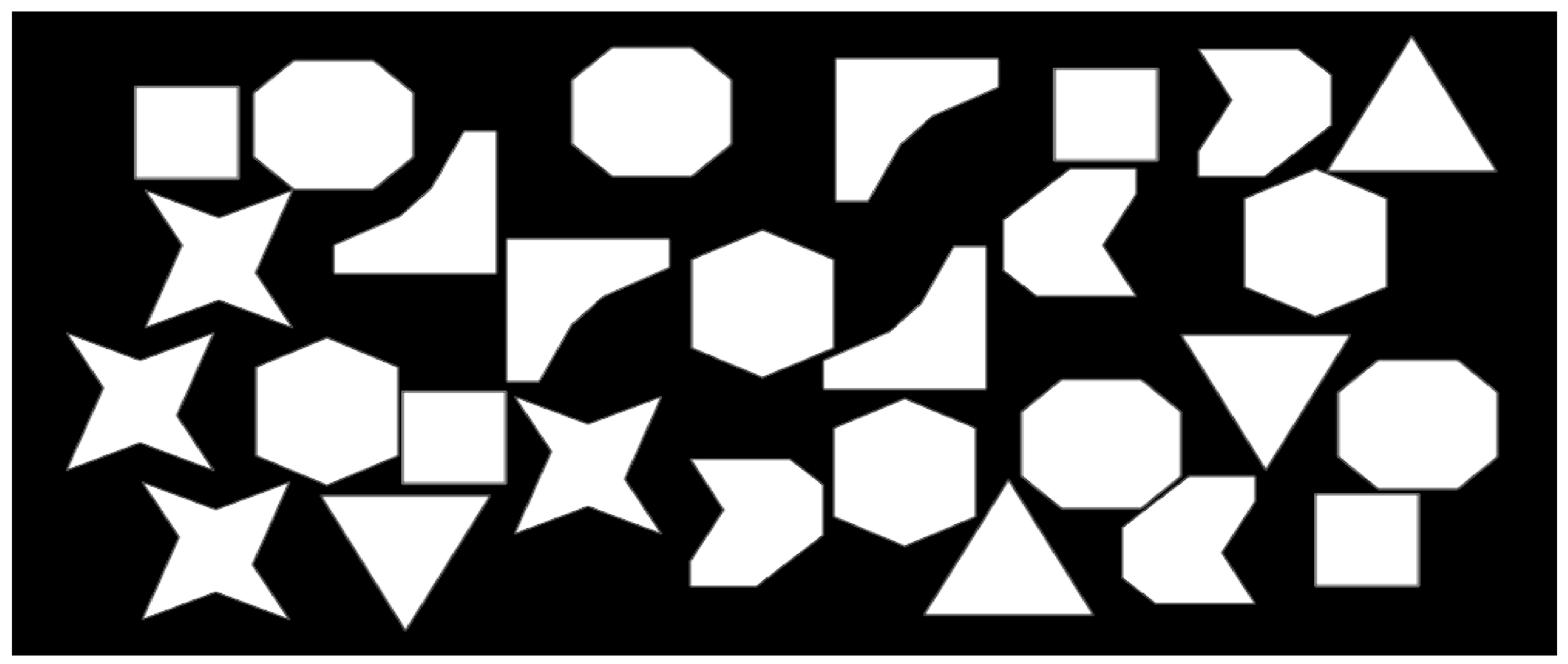
For the initial ILS tests, amorphous pieces, such as those presented in Figure 2, were used. Figure 4 depicts the landscape behavior of 500 tests carried out, each one consuming 500 seconds. The parameters shown are (1) shapes (the number of pieces placed on the PPA), (2) residual area, and (3) overlaps (the number of overlaps generated). The red rectangle in Figure 4 encloses the best solutions found using a high number of attempts (based on the number of checked overlaps before reaching a feasible solution). This figure also shows a portion enclosed in a grid of black lines, indicating the best values reached using the fewest attempts. These values ranged between 48 and 50 for the number of pieces placed on the PPA. ILS obtained the best solution when the objective function with 50 pieces was placed on the PPA.

It is interesting to see the difficulty degree of obtaining feasible solutions. Suppose the solutions had a more significant number of pieces inserted on the PPA. In that case, ILS could generate many overlaps before finding improved solutions. However, the best solutions found generated close to 500,000 to 1,500,000 overlaps. In contrast, solutions with a lower value (marked in Figure 4 with a red rectangle) used 46 and 47 pieces and detected close to 3,500,000 overlaps. This result is interesting since it points out that a local search finds a better trajectory in the solution space, avoiding further exploration of the best solutions.

Table 1. ILS results of 500 experimental tests.

Time = 500 s
Solution Quality	Number of Pieces	Residual Area (Pixels)
Best solution	50	620,940
Worst solution	42	678,876
Mean	46	649,908
Mode	45	657,150

shows the best and worst values and the mean and mode of the objective function values. The PPA value was 983,040 square pixels. The area of each piece was 7242 square pixels. The best solution obtained from the implemented algorithm’s objective function represents 63.16% of the occupation area. This data was obtained considering the pieces inserted on the PPA and the PPA without pieces.

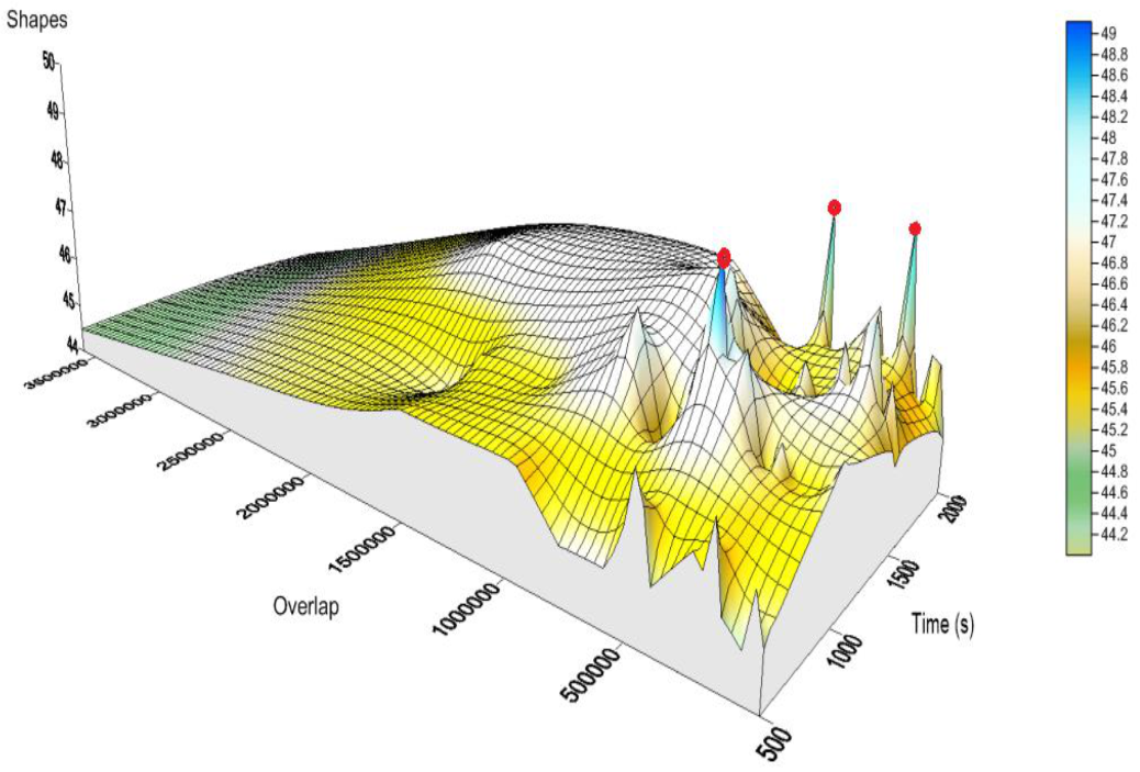
Figure 5 shows the landscape behavior as a function of time. This graph is based on the number of pieces, the number of overlaps, and the execution time in seconds, using 120 experimental tests.

The total ILS iterations are 10,000. The best solutions obtained are within the range of 100,000 to 1,500,000 overlaps, with 1000 and 2000 s of execution time, as shown in Figure 5. The red dots identify the best solutions on the figure. It can be seen that the worst solutions were when the number of overlaps increased until approximately 2,000,000 overlaps. Peaks and valleys are observed in the figure, representing the best and worst solutions, respectively. This behavior indicates that the quality increase is not directly or inversely proportional to the ILS execution time. It is observed that bad solutions in the landscape surround the best solutions. This behavior indicates that the ILS execution can find good solutions in each of its executions.

Table 2. ILS behavior with different executions times.

Time = 500 s		Time = 1000 s
Solution Quality	Number of Pieces	Solution Quality	Number of Pieces
Best solution	48	Best solution	50
Worst solution	44	Worst solution	45
Mean	45	Mean	46
Mode	45	Mode	46

and

Table 3. ILS behavior with different executions times.

Time = 1500 s		Time= 2000 s
Solution Quality	Number of Pieces	Solution Quality	Number of Pieces
Best solution	50	Best solution	49
Worst solution	45	Worst solution	43
Mean	46	Mean	46
Mode	45	Mode	47

show a summary of all results obtained by the implemented algorithm.

From the values in Table 2 and Table 3, it can be concluded that the best solutions obtained by the algorithm were in the time intervals between 1000 and 1500 s, with 50 pieces. However, in the time interval of 2000 s, a solution of 49 pieces was found.

The graph in Figure 6 shows the landscape behavior as a function of time.

In Figure 3, the behavior of the parameters on 120 experimental tests is represented. In this figure, bad solutions can be distinguished based on the largest residual area, which stands out in the landscape peaks. The worst and best solutions are displayed in the landscape using yellow and red dots, respectively. It can be seen that the worst solutions increased the number of overlaps to about 2,000,000. A black point in Figure 6 identifies the worst solution obtained by the objective function. This point is located on the upper right corner of the graph, specifically where the blue part of the landscape with the worst solutions is located. The algorithm behavior is considered variably since the surface describes an irregular landscape where the best solutions are found. The total iterations were 10,000.

Table 4. ILS behavior with different execution times (residual area).

Time = 500 s		Time = 1000 s
Solution Quality	Residual Area	Solution Quality	Residual Area
Best solution	635,424	Best solution	620,940
Worst solution	664,392	Worst solution	657,150
Mean	657,150	Mean	649,908
Mode	657,150	Mode	649,908

and

Table 5. ILS behavior with different execution times (residual area).

Time = 1500 s		Time = 2000 s
Solution Quality	Residual Area	Solution Quality	Residual Area
Best solution	620,940	Best solution	628,182
Worst solution	657,150	Worst solution	671,634
Mean	649,908	Mean	649,908
Mode	657,150	Mode	642,666

represent a summary of the results obtained by the objective function. It is observed that the best and the worst values are 620,940 and 671,634 square pixels, respectively. The best solutions found in the time intervals of 1000, 1500, and 2000 s were 620,940, 620,940, and 628,182 square pixels, respectively, with 63.13% and 63.90% of the PPA used. In these intervals, the algorithm consumed more time applying perturbation movements to exploiting the solutions space.

Comparative tests of the ILS algorithm were performed with other algorithms proposed in the existing literature, using the following benchmark instances [2]: Shapes 0, Shapes 1, Shapes 2, Shirts, and Swim.

Table 6. Pieces used in each benchmark instance.

Instance	Piece
	1	2	3	4	5	6	7	8	9	10
Shapes 0
Shapes 1
Shapes 2
Shirts
Swim

presents the pieces in each instance. For the Shape 0 instance, 4 different shapes were required. For the Shape 1 instance, 6 different shapes were required. For the Shape 2 instance, 7 different shapes were required. For the Shirts instance, 8 different shapes were required, and for the Swim instance, 10 different shapes were required. The sizes of each figure used for ILS testing were the same. Note that no amorphous shapes were used in these instances, and studies in the existing literature with comparable results did not use rotational movements either. They placed the pieces to build sets with different orientations (0°, 90°, 180°, and 270°) before inserting them into the bin. In the algorithm proposed in this paper, some figures were rotated before introducing them to ILS to match the solution presented in the existing literature, since in this work, ILS does not handle figure rotation.

Table 7. Time used to find the same solution using different algorithms.

Instance	Algorithms
	CA [2]	PHNFP [5]	FF [8]	HSDM [11]	ILS
	Time (s)
Shapes 0	34.6	7.8	14	263.7	1106
Shapes 1	23.3	360	19	408.3	1560
Shapes 2	10.9	223.8	1	60.7	1952
Shirts	210.5	168.6	97	618.3	1603
Swim	---	535.6	121	1988.1	2079

presents the comparative tests of ILS with other algorithms in the existing literature, including the Constructive Algorithm (CA) [2], the Placement Heuristic with Not-Fit-Polygon (PHNFP) [5], the First Fit algorithm (FF) [8], and the Heuristic Search Diversification Mechanism (HSDM) [11]. In these methods, the number of pieces is kept constant and the paper size is reduced until the same number of pieces can no longer be inserted. In the case of the ILS procedure, the paper size is kept constant (40 × 80 units). To use pixels, a transformation of those dimensions from world coordinates to screen coordinates is conducted to obtain the sheet size in pixels, which is 625 × 1250, with a total sheet area of 781,250 pixels. It is observed in this table that ILS takes more time than the others to find the same solution. This behavior is due to the fact that the overlap detection algorithm used by ILS must be generating the mask of each piece moving in the PPA to find a new neighboring solution s’. This algorithm always considers amorphous pieces even if they are not present. Therefore, it was necessary to evaluate the pixels mask representing the piece for overlapping detection. However, the solutions presented in Table 7 of each instance were found. As the ILS algorithm does not have some rotation procedure, the pieces were previously rotated to be used in the algorithm to compare the results with those described in the existing literature. For example, in Shape 1 instance shown in Table 6, 4 pieces of type 5 were used and 2 pieces (5 and 6) were rotated before introducing them to the algorithm. It has been established that in future work, the pieces will rotate at any angle to improve the ILS algorithm efficiency.

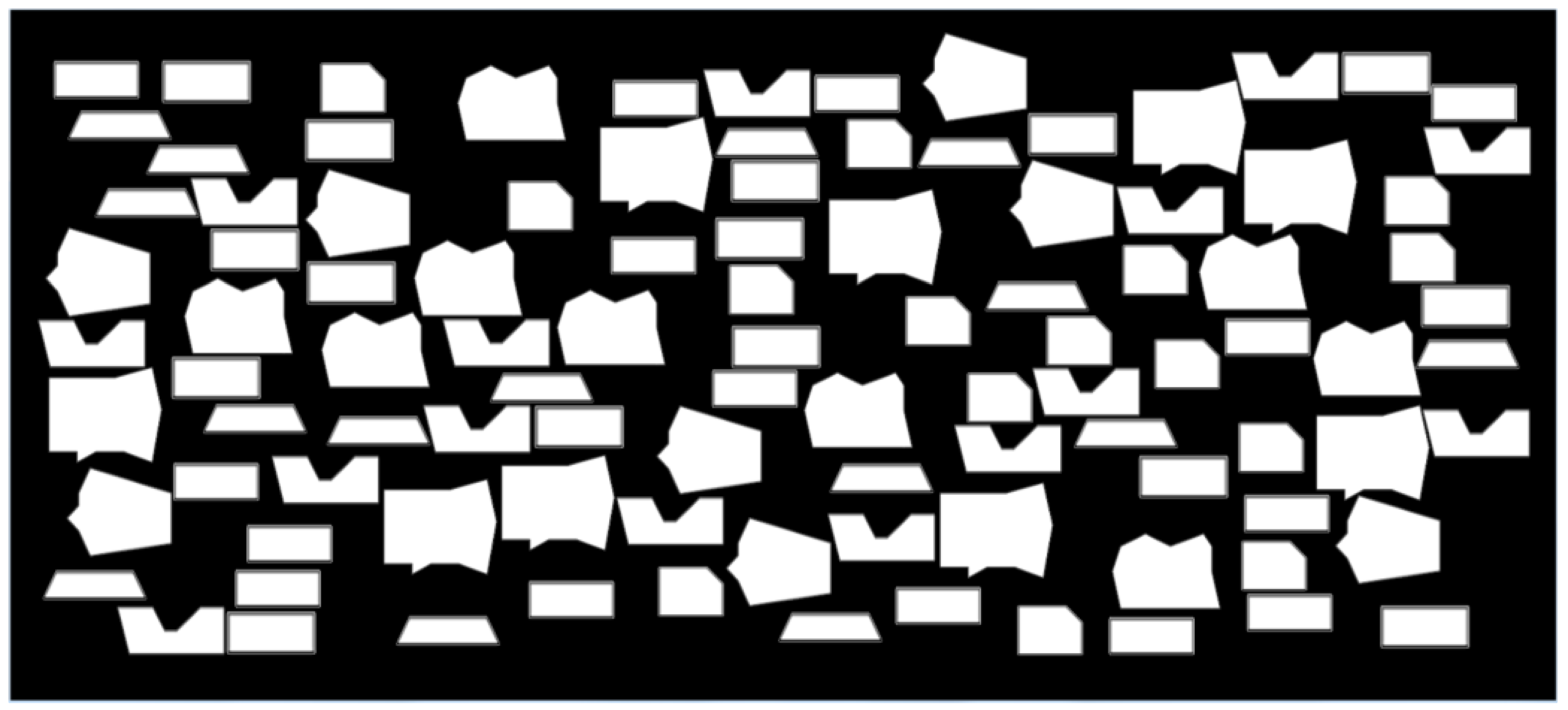
Figure 7, Figure 8, Figure 9, Figure 10 and Figure 11 present the solution for the five instances. These are the same as those found for the compared algorithms. However, the locations of the pieces in the PPA were naturally different and the residual area was huge.

Table 8. ILS results for each benchmark instance consuming 2 h of processing time.

Instance	Maximum	Minimum	Mode	%RA	%RAOp
Shapes 0	49	47	48	65.72	61.10
Shapes 1	48	47	48	65.72	61.48
Shapes 2	31	30	31	38.74	36.78
Shirts	101	100	101	57.75	56.92
Swim	51	50	51	69.45	66.52

presents the optimized ILS tests with the benchmark instances of Table 6 based on a time limit of two hours, keeping the sheet size constant and increasing the number of inserted pieces. There were 30 tests performed for each instance, and the best, worst, and mode solutions are presented. ILS could insert more pieces in the same sheet size if the time increased to 2 h. However, the percentage of residual area was still huge (between 36.78% to 66.52%). It is not possible to compare the results of other methods described in the existing literature, since they reduce the bin area using a constant number of pieces to be inserted. Alternatively, the method proposed in this study was used to optimize the paper waste in digital printers where the paper area was constant. However, if irregular pieces with few concavities were used, the results of other authors were better than the method proposed in this work. RA is the residual area in percentage, and RAOp is the optimized residual area in percentage, both measured in square pixels.

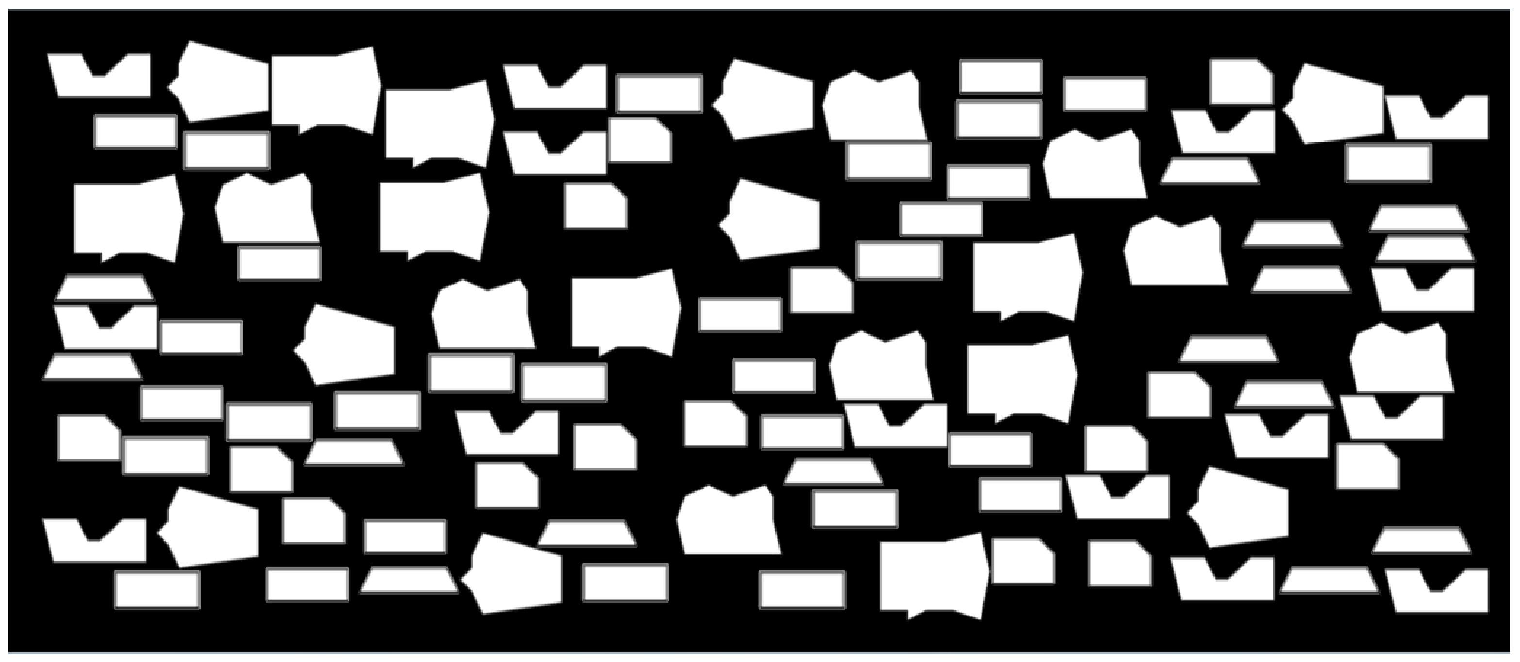
Figure 12, Figure 13, Figure 14, Figure 15 and Figure 16 show the ILS algorithm’s solution for each instance with 2 h of processing time. In each figure, can be observed that several pieces presented an approach within the mask of inactive pixels. This allowed for a better approach without overlapping the pieces’ edges (regular, irregular, amorphous, or a combination). This behavior can allow for a more significant number of piece insertions when amorphous pieces are used.

Each piece used in the instances described in Table 6 had a reduced number of vertices and few concavities. The complexity to compute overlaps in two convex pieces, A and B, is O(nm), where n and m are the number of vertices of A and B, respectively. Concavities found in concave polygons are a challenge to avoiding overlap between them, and are more difficult when there are a large number of concavities in the pair of pieces A and B. This problem has been dealt with in the literature by dividing each piece into convex polygons, which are simpler to deal with. A different approach is to slide a reference point of piece B around the circumference of piece A. Another approach uses diagrams, where the slope is computed only in the piece concavities requiring special treatment [19]. The methods to overlap detection between a pair of pieces using trigonometric calculations have one increased time complexity to detect overlaps in irregular pieces when the number of concavities and vertices is increased. In this work, ILS generated a mask with the Allegro software for each inserted piece and used the CheckOverlaps function of Algorithm 2, avoiding the use of trigonometric. Because no instances with amorphous pieces were found in the literature to be able to make comparisons with ILS, in this work, instances containing amorphous pieces were proposed.

Table 9. Amorphous pieces used in each instance.

Instance	Piece
	1	2	3	4	5	6	7	8
A0
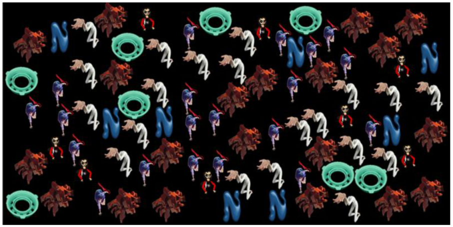
A1
A2
A3

shows the instances proposed in this paper using amorphous figures. These figures have a huge number of vertices and concavities that are commonly printed in digital printers. Instances A0-A3 presented different piece designs to be able to evaluate the ILS procedure and check if the residual area increased according to the complexity of the inserted figures, depending on their vertices and concavities. Instance A0 showed several figures with pronounced concavities and a large number of vertices.

Table 10. ILS results for each benchmark instance consuming 2 h of processing time.

Instance	Maximum	Minimum	Mode	%RAOp
A0	41	39	40	59.60
A1	84	80	80	66.30
A2	73	70	72	61.24
A3	78	77	77	56.97

presents the ILS results of running the algorithm for 2 h for each instance with amorphous pieces. There were 30 tests conducted for each instance. We observed that the residual area RAOp obtained for the four instances was similar to that obtained for the instances that handled few vertices and reduced concavities (Table 8), except for Shape 2, where the inserted pieces had a larger area, allowing for better optimization of the RAOp. This behavior indicates that the execution of ILS does not have a visible effect when the number of vertices and concavities in the pieces to be inserted is high.

Figure 17, Figure 18, Figure 19 and Figure 20, show the solution of the ILS algorithm for A0–A4 instances with 2 h of running time. We performed a comparison of the RAOp results with the instances presented in the literature with irregular pieces (Table 8) and the proposed instances of amorphous pieces (Table 10). From Table 8, for the Shape 2 instance, where the RAOp was 36.78%, it can be seen (Figure 14) that the pieces were larger than the other instances in Table 8, indicating that when ILS inserts larger figures, it works more efficiently. If we see instance A0 (Table 10), which obtains one of the best RAOp, it is observed (Figure 17) that the figures were a little larger than instances A1 to A3, but we can also see that instance A3 obtained the best RAOp and presented the largest number of different pieces to insert. This behavior indicates that ILS works better when a greater number of different pieces are inserted and when they have a greater number of vertices and concavities.

For conducting the statistical analysis, both data normality and homoscedasticity were first verified. The test data were the run times (Table 7) to obtain the same results in each evaluated algorithm (PHNFP, FF, HSDM, and ILS). The null hypothesis, $H_0$ in Equation (11), indicates that the means of the results are equal. The alternative hypothesis, Equation $H_1$ in (12), points out that the means are not equal, or at least one is different.

$$H_0:\overline{X_1}=\overline{X_2}=\dots =\overline{X_r}$$

(11)

$$H_1:Not all are the same$$

(12)

Figure 21 shows no normality for the data since the points are not located on the graph’s diagonal.

The homoscedasticity analysis is shown using the box-and-whisker graphs presented in Figure 22. It can be seen that the boxes for each algorithm are not equal, so a difference in variances can be admitted, which indicates that homoscedasticity cannot exist. As the normality and homoscedasticity of the data do not exist, the parametric ANOVA test could not be used. Thus, a robust ANOVA with the Welch and Box tests [20] was used.

Welch’s test, defined by Equations (13)–(23), uses weights w_i to reduce the data heterogeneity. The weights w_i in Equation (13) are based on the sample size n_i of the data generated by the i-th algorithm and the observed variance s²_w,_i for each i-th group of data generated by the i-th algorithm. For the i-th group of data generated by the i-th algorithm,

$$d_i=\frac{\left(n_i-1\right)s_{w,i}^2}{h_i\left(h_i-1\right)}$$

(13)

where n_i is the sample size of the i-th algorithm, s²_w,_i is the winsorized variance (of the trimmed data), h_i is the adequate sample size of the i-th group (number of observations remaining after the cut-off).

$$w_i=\frac{1}{d_i}$$

(14)

$$U={\displaystyle \sum }_{i=1}^r{w}_i$$

(15)

$$\overline{X}=\frac{1}{U}{\displaystyle \sum }_{i=1}^r{w}_i{\overline{x}}_{\alpha .i}$$

(16)

where ${\overline{\mathit{x}}}_{\mathit{\alpha }\mathbf{.}\mathit{i}}$ are the trimmed means.

$$A=\frac{1}{r-1}{\displaystyle \sum }_{i=1}^r{w}_i{\left({\overline{x}}_{\alpha .i}-\overline{X}\right)}^2$$

(17)

$$B=\frac{2\left(r-2\right)}{r^2-1}{\displaystyle \sum }_{i=1}^r\frac{{\left(1-\frac{w_i}{U}\right)}^2}{h_i-1}$$

(18)

$$F_{w=\frac{A}{1+B}}$$

(19)

From the Fw statistic, if H₀ is true, then a Snedecor Fw distribution with v₁ and v₂ degrees of freedom is used, where

$$v_1=r-1$$

(20)

$$v_2=\frac{2r-4}{3B}$$

(21)

Then, the decision rule to control the significance level α is

$$H_o\mathrm{is} \mathrm{accepted} \mathrm{if} F_w\le F_{\left(1-\alpha ;v_1,v_2\right)}$$

(22)

$$H_o \mathrm{is} \mathrm{refused} \mathrm{if} F_w>F_{\left(1-\alpha ;v_1,v_2\right)}$$

(23)

If H_o is true, the F_w statistic follows a Snedecor probability distribution with $\left(1-\alpha ;v_1,v_2\right)$ degrees of freedom.

The robust generalization of the Box test is presented in (24)–(27), where the F_w statistic is as follows:

$$F_w=\frac{{\displaystyle \sum }_{i=1}^r{h}_i{\left({\overline{x}}_{\alpha .i}-\overline{x}\right)}^2}{{\displaystyle \sum }_{i=1}^r\left(1-\frac{h_i}{H}\right)S_i^2}$$

(24)

where

$$H={\displaystyle \sum }_{i=1}^r{h}_i$$

(25)

$$\overline{x}=\frac{{{\displaystyle \sum }}_{i=1}^r{h}_i{\overline{x}}_{\alpha ,i}}{H}$$

(26)

$$S_i^2=\frac{\left(n_i-1\right)s_{w,i}^2}{h_i-1}$$

(27)

The null hypothesis is rejected for large values of the F_w statistic. If the null hypothesis is accepted, it follows a Snedecor F-distribution with the following freedom degrees:

$$v_1=\frac{{\left({{\displaystyle \sum }}_{i=1}^r\left(1-f_i\right)S_i^2\right)}^2}{{\left({{\displaystyle \sum }}_{i=1}^r{S}_i^2{f}_i\right)}^2+{{\displaystyle \sum }}_{i=1}^r{S}_i^4\left(1-2f_i\right)}$$

(28)

$$v_2=\frac{{\left({{\displaystyle \sum }}_{i=1}^r\left(1-f_i\right)S_i^2\right)}^2}{\frac{{{\displaystyle \sum }}_{i=1}^r{S}_i^4{\left(1-f_i\right)}^2}{\left(h_i-1\right)}}$$

(29)

where

$$f_i=\frac{h_i}{H}$$

(30)

In this work, the statistical analysis was carried out using the robust ANOVA test, defined in Equations (12)–(23) with Welch’s test and (24)–(30) with Box’s.

Welch was implemented in the t1way (x, tr, grp) function of the WRS R package [21]. In the t1way function, x is the data, tr is the trimmed means, and grp indicates the subset size to be compared. In this case, 4 algorithms were compared using 10% of the trimmed means. A p-value of 3.315954 × 10⁻⁴ was obtained. The null hypothesis was refused since there were differences between the algorithms’ trimmed means. The F_w value was 26.45909, and the freedom degrees were v₁ = 3, and v₂ = 7.039397, with $1-\alpha$ = 0.95, the v₁ and v₂ values, Fisher table values [22], and a Snedecor value of 4.347. Since $26.45909>{4.347}_{\left(0.95;3,7.039397\right)}$, the H0 was refused, indicating that differences in the trimmed means existed.

The robust generalization of the Box test was implemented with tr = 10% in the box1way (x, 0.1) function of the WRS R package [21]. A p-value of 6.406586 × 10⁻³ was obtained, F_w was 13.219, and v₁ and v₂ were 1.527593 and 6.5418, respectively. The Snedecor value was 7.322 and the null hypothesis was refused ($26.45909>{4.347}_{\left(0.95;3,7.039397\right)}$). These values indicate that differences existed between the behaviors of the analyzed algorithms.

5. Conclusions

It can be understood that the neighborhood structure developed in this work operates effectively and efficiently since it detects and corrects the overlaps between regular, irregular, and amorphous figures. According to the landscape analysis, this structure can optimize the solution by finding better ones not depending proportionally on the overlaps generated. Moreover, it does not present a clear proportionality as a function of time. This behavior implies that the increase in a much greater execution time of ILS does not always improve the solution. The comparison with other algorithms in the existing literature using regular and irregular figures shows the ILS effectiveness in finding the same solutions. Statistical tests show that differences between the behavior of the compared algorithms exist.

The contribution of this paper is to apply the 2D BPP to solve the paper waste reduction problem in digital printing presses with amorphous shapes. This approach creates models where the figures are distributed on the printable paper area and can reduce the residual area. The figures used in digital printing presses are of all kinds (regular, irregular, amorphous, and combinations of these).

In future research, it is crucial to improve the ILS execution time to make it more efficient and significantly reduce the residual area RAOp. One proposal is to parallelize the overlap detection algorithm to speed up reading the masks’ pixels that detect overlaps. Works with distributed processing have been done using cloud computing to solve the bin packing problem [23]. To reduce the residual area, the developed neighborhood structure can also be improved by applying movements such as insertion in pairs of figures, translation, rotation, and a combination of these movements. This has already been done in other works and is known as a variable neighborhood [24]. More regular, irregular, and amorphous figures can be inserted into the paper sheet with these perturbations, generating more significant space for new solutions and greater movements in the neighborhood structure. An important point is the rotation treatment, an orientation of the figures at different angles before inserting them into the paper sheet, which is already included in the literature. We will handle, in future work, the rotation of figures already inserted in the paper sheet, with the possibility of rotating the figure at random, which we think can give greater efficiency to the neighborhood variable that will be designed.

References

1. Garey, M.R.; Johnson, S.S. Computers and Intractability a Guide to the Theory of NP-Completeness; Freeman: New York, NY, USA, 1979; ISBN 0-7167-1044-7. [Google Scholar]
2. Oliveira, J.F.; Gomes, A.M.; Ferreira, J.S. TOPOS—A new constructive algorithm for nesting problems. OR-Spektrum 2000, 22, 263–284. [Google Scholar] [CrossRef]
3. Bennell, J.A.; Oliveira, J.F. The geometry of nesting problems: A tutorial. Eur. J. Oper. Res. 2008, 184, 397–415. [Google Scholar] [CrossRef]
4. Bennell, J.A.; Oliveira, J.F. A tutorial in irregular shape packing problems. J. Oper. Res. Soc. 2009, 60, S93–S105. [Google Scholar] [CrossRef]
5. Bennell, J.A.; Song, X. A beam search implementation for the irregular shape packing problem. J. Heuristics 2010, 16, 167–188. [Google Scholar] [CrossRef] [Green Version]
6. Han, W.; Bennell, J.A.; Zhao, X.; Song, X. Construction heuristics for two dimensional irregular shape bin packing with guillotine constraints. Eur. J. Oper. Res. 2013, 230, 495–504. [Google Scholar] [CrossRef] [Green Version]
7. López-Camacho, E.; Ochoa, G.; Terashima-Marin, H.; Burke, E.K. An effective heuristic for the two-dimensional irregular bin packing problem. Ann. Oper. Res. 2013, 206, 241–264. [Google Scholar] [CrossRef] [Green Version]
8. Martinez-Sykora, A.; Alvarez-Valdes, R.; Bennell, J.A.; Ruiz, R.; Tamarit, J.M. Metaheuristics for the irregular bin packing problem with free rotations. Eur. J. Oper. Res. 2017, 258, 440–455. [Google Scholar] [CrossRef] [Green Version]
9. Johnson, D.S.; Demers, A.; Ullman, J.D.; Garvey, M.R.; Graham, R.L. Worst-case performace bounds for simple one-dimensional packing algorithms. SIAM J. Comuting 1974, 3, 299–325. [Google Scholar] [CrossRef] [Green Version]
10. López-Camacho, E.; Terashima-Marin, H.; Ross, P.; Ochoa, G. A unified hyper-heuristic framework for solving packing problems. Expert Syst. Appl. 2014, 41, 6876–6889. [Google Scholar] [CrossRef]
11. Abeysooriya, R.P.; Bennell, J.A.; Martinez-Sykora, A. Jostle heuristics for the 2D-irregular shapes bin packing problems with free rotation. Int. J. Prod. Econ. 2018, 195, 12–26. [Google Scholar] [CrossRef] [Green Version]
12. Chernov, N.; Stoyan, Y.; Romanova, T. Mathematical model and efficient algorithms for objects packing problem. Comput. Geom. Theory Appl. 2010, 43, 535–553. [Google Scholar] [CrossRef] [Green Version]
13. Wäscher, G.; Haußner, H.; Schumann, H. An improved typology of cutting and packing problems. Eur. J. Oper. Res. 2007, 183, 1109–1130. [Google Scholar] [CrossRef]
14. Dyckhoff, H. A typology of cutting and packing problems. Eur. J. Oper. Res. 1990, 44, 145–159. [Google Scholar] [CrossRef]
15. Lourenco, H.R.; Martin, O.; Stützle, T. A beginner´s introduction to iterated local search. In Proceedings of the MIC2001: 4th Metaheuristics International Conference, Porto, Portugal, 16–20 July 2001; pp. 1–6. [Google Scholar]
16. Handbook of Metaheuristics, Chapter Iterated Local Search; Lourenço, H.R.; Martin, O.C.; Stützle, T.; Kochenberger, G. (Eds.) Kluwer Academic Publishers: Norwell, MA, USA, 2002; pp. 321–353. [Google Scholar]
17. Salto, C. Meta heurísticas Híbridas paralelas para problemas industriales de corte, empaquetado y otros relacionados. In Proceedings of the WICC2010: XII Workshop de Investigadores en Ciencias de la Computación, Comodoro Rivadavia, Argentina, 5–6 May 2010; pp. 822–831. [Google Scholar]
18. Papadimitriou, C.H.; Steiglitz, K. Combinatorial Optmization. Algorithms and Complexity; Dover Publication: Mineola, NY, USA, 1998; ISBN 0-486-40258-4. [Google Scholar]
19. Dowsland, K.A.; Dowsland, W.B.; Bennell, J.A. Jostling for position: Local improvement for irregular cutting patterns. J. Oper. Res. Soc. 1998, 49, 647–658. [Google Scholar] [CrossRef]
20. Wilcox, R. Introduction to Robust Estimation and Hypothesis Testing, 3rd ed.; Academic Press: Cambridge, MA, USA, 2013; ISBN 9780123869838. [Google Scholar] [CrossRef]
21. R Version 4.0.5. Copyright ©, The Foundation for Statistical Computing. Available online: https://cran.r-project.org/bin/windows/base/ (accessed on 31 March 2021).
22. Guenther, W. Introducción a la Inferencia Estadística, 1st ed.; McGraw-Hill: Panama, PA, South America, 1977; ISBN 978-84-219-0061-1. 357p. [Google Scholar]
23. Aydın, N.; Muter, I.; Birbil, I. Multi-objective temporal bin packing problem: An application in cloud computing. Comput. Oper. Res. 2020, 121, 104959. [Google Scholar] [CrossRef]
24. Baioletti, M.; Milani, A.; Santucci, V. Variable neighborhood algebraic differential evolution: An application to the linear ordering problem with cumulative costs. Inf. Sci. 2020, 507, 37–52. [Google Scholar] [CrossRef]
Figure 1. Mockup design for the digital printing of pieces with diverse sizes.
Mathematics 09 01033 g001
Figure 2. Neighborhood structure from the movements of the figures. (a) Piece F (yellow color), chosen in a solution s. (b) F movement, modifying its coordinates. (c) New piece G (red color) inserted in s generates s′.
Mathematics 09 01033 g002
Figure 3. ILS flow diagram to the paper waste optimization problem.
Mathematics 09 01033 g003
Figure 4. ILS landscape average of 500 tests (shapes, overlaps, and residual area).
Mathematics 09 01033 g004
Figure 5. ILS landscape average of 120 tests (shapes, overlaps, and time).
Mathematics 09 01033 g005
Figure 6. ILS landscape average of 120 tests (residual area, overlaps, and time).
Mathematics 09 01033 g006
Figure 7. Solution found by the ILS algorithm using 43 pieces for the Shape 0 instance.
Mathematics 09 01033 g007
Figure 8. Solution found by the ILS algorithm using 43 pieces for the Shape 1 instance.
Mathematics 09 01033 g008
Figure 9. Solution found by the ILS algorithm using 28 pieces for the Shape 2 instance.
Mathematics 09 01033 g009
Figure 10. Solution found by the ILS algorithm using 99 pieces for the Shirts instance.
Mathematics 09 01033 g010
Figure 11. Solution found by the ILS algorithm using 48 pieces for the Swim instance.
Mathematics 09 01033 g011
Figure 12. Solution found by the ILS algorithm inserting 49 pieces for the Shape 0 instance, consuming 2 h of processing time.
Mathematics 09 01033 g012
Figure 13. Solution found by the ILS algorithm inserting 48 pieces for the Shape 1 instance, consuming 2 h of processing time.
Mathematics 09 01033 g013
Figure 14. Solution found by the ILS algorithm inserting 31 pieces for the Shape 2 instance, consuming 2 h of processing time.
Mathematics 09 01033 g014
Figure 15. Solution found by the ILS algorithm inserting 101 pieces for the Shirts instance, consuming 2 h of processing time.
Mathematics 09 01033 g015
Figure 16. Solution found by the ILS algorithm inserting 51 pieces for the Swim instance, consuming 2 h of processing time.
Mathematics 09 01033 g016
Figure 17. Solution found by the ILS algorithm when inserting 50 pieces for the A0 instance, consuming 4 h of processing time.
Mathematics 09 01033 g017
Figure 18. Solution found by the ILS algorithm when inserting 84 pieces for the A1 instance, consuming 4 h of processing time.
Mathematics 09 01033 g018
Figure 19. Solution found by the ILS algorithm when inserting 73 pieces for the A2 instance, consuming 4 h of processing time.
Mathematics 09 01033 g019
Figure 20. Solution found by the ILS algorithm when inserting 71 pieces for the A3 instance, consuming 4 h of processing time.
Mathematics 09 01033 g020
Figure 21. Normality graphs for PHNFP, FF, HSDM, and ILS algorithms.
Mathematics 09 01033 g021
Figure 22. Box-and-whisker graphs for PHNFP, FF, HSDM, and ILS algorithms.
Mathematics 09 01033 g022