Control Method of Flexible Manipulator Servo System Based on a Combination of RBF Neural Network and Pole Placement Strategy

Abstract

Gravity and flexibility will cause fluctuations of the rotation angle in the servo system for flexible manipulators. The fluctuation will seriously affect the motion accuracy of end-effectors. Therefore, this paper adopts a control method combining the RBF (Radial Basis Function) neural network and pole placement strategy to suppress the rotation angle fluctuations. The RBF neural network is used to identify uncertain items caused by the manipulator’s flexibility and the time-varying characteristics of dynamic parameters. Besides, the pole placement strategy is used to optimize the PD (Proportional Differential) controller’s parameters to improve the response speed and stability. Firstly, a dynamic model of flexible manipulators considering gravity is established based on the assumed mode method and Lagrange’s principle. Then, the system’s control characteristics are analyzed, and the pole placement strategy optimizes the parameters of the PD controllers. Next, the control method based on the RBF neural network is proposed, and the Lyapunov stability theory demonstrates stability. Finally, numerical analysis and control experiments prove the effectiveness of the control method proposed in this paper. The means and standard deviations of rotation angle error are reduced by the control method. The results show that the control method can effectively reduce the rotation angle error and improve motion accuracy.

1. Introduction

Flexible manipulators are complex systems with multiple inputs and multiple outputs. They are widely used in in-depth space exploration, industrial assembly, and other fields [1,2]. Compared with the traditional rigid manipulators, flexible manipulators have a larger radius of rotation and lighter weight. Flexible manipulators are more likely to vibrate in a low-frequency area. In order to clarify the reasons for the vibration of flexible manipulators, it is necessary to carry out a dynamic modeling analysis. At present, the modeling methods of flexible manipulators are mainly divided into two categories. One is the finite element (FE) method, and the other is the assumed mode method (AMM). In literature [3,4,5], the dynamic equations of flexible manipulators with the rotation angle coupled with modal coordinates are established by using the AMM. In literature [6], the FE method is used to establish the dynamic equation of flexible manipulators with flexible joints. Compared with the AMM, the FE method is more suitable for flexible manipulators with irregular shapes [7]. Nowadays, in the dynamic modeling processes of flexible manipulators, it is usually assumed that flexible manipulators move in the horizontal plane, as shown in the literature [8,9]. According to this assumption, the influence of gravity on flexible manipulators can be ignored. However, in some practical applications of flexible manipulators, the gravity factor needs to be considered [2,10]. In literature [11], the gravity factor is considered in modeling processes of the servo system for a manipulator with flexible joints. Gravity is introduced into the dynamic equation as a strong nonlinear term. Therefore, the gravity factor needs to be considered in the dynamic modeling of flexible manipulators.

The control methods of the servo system for flexible manipulators mainly include active control and passive control. The active control method is to obtain stable output by changing controller parameters or controller structures. The passive control method is to eliminate the resonant influence of the flexible manipulators by adding a notch device. The active control methods mainly include PID (Proportional Integral Differentiation) control [12,13], sliding mode control [14,15], robust control [16,17], etc. In literature [13], the nonlinear self-tuning PID controller is used to control the flexible manipulators. In literature [15], the sliding mode controller with observer is used to control the angle of manipulators. In literature [16], the linear quadratic Gaussian and the weighted H infinity controller are adopted to control flexible manipulators. Compared with rigid manipulators, the nonlinear flexible factor is introduced into the dynamic equation of flexible manipulators. This kind of flexible nonlinear factor brings difficulty to the design of the servo system controller. If the gravity factor is considered in flexible manipulators’ dynamic modeling processes, the nonlinear factor is introduced again. This further increases the difficulty of the servo system controller design. In literature [18], internal control loops with nonlinear terms are added to compensate for the influence of gravity factors on rigid manipulators. There are some uncertain items in the servo system for flexible manipulators. These uncertain items come from the errors in the dynamic modeling processes and the parameters’ time-varying characteristics during the motion of flexible manipulators. Neural networks are widely used in the identification of system uncertain items. Literature [19,20] uses the neural network to identify the uncertain items in the dynamic system of flexible-joint manipulators, thus improving the control precision. Therefore, the neural network can be used to identify the uncertain items in the dynamic system of flexible manipulators. Then, the input torque can be compensated in the way of an internal control loop. Besides, the controller parameters also affect the output of the servo system for flexible manipulators. In literature [21,22], the controller parameters are optimized by adjusting the pole coefficients, and the rigid manipulators obtain a good output.

According to the literature [23,24], a flexible manipulator is equivalent to a flexible beam model in this paper. The dynamic equation of the servo system for flexible manipulators is established by using the AMM. Gravity is taken into account in the modeling of dynamics. Then the transmission of the servo system for flexible manipulators is analyzed through dynamic equations. The controller parameters of the servo system also affect the output accuracy. In this paper, a pole placement strategy is used to optimize the controller parameters. Then, the RBF neural network is used to identify the uncertain items of the servo system for flexible manipulators. Among them, the servo system’s uncertain items are composed of the parameter time-varying part and the flexible part. After the neural network identification, it is compensated into the control system again in the way of an internal control loop. Therefore, the accuracy of the input torque of the servo system is improved. This paper’s main contribution is to improve the control accuracy by using a combination of pole placement strategy and neural network. The RBF neural network is used to identify uncertain items containing flexible factors. The gravity factor’s influence is considered in the modeling processes, and the gravity item in the dynamic equation is compensated through the internal control loop.

The rest of the paper is organized as follows: Section 2 establishes the dynamic equation of the servo drive system for flexible manipulators with gravity found using the AMM and Lagrange’s principle. Section 3 describes the servo system’s control characteristics and uses the PD control strategy based on the pole placement strategy to control the position loop. Section 4 uses the PD control strategy based on the RBF neural network to control the servo system, and the stability of the servo system’s is proved by Lyapunov stability theory. Section 5 carries out the numerical simulation and experiments of flexible manipulators to verify the proposed control strategy’s effectiveness. Section 6 states the conclusion.

2. Dynamic Modeling of the Flexible Manipulator Servo System

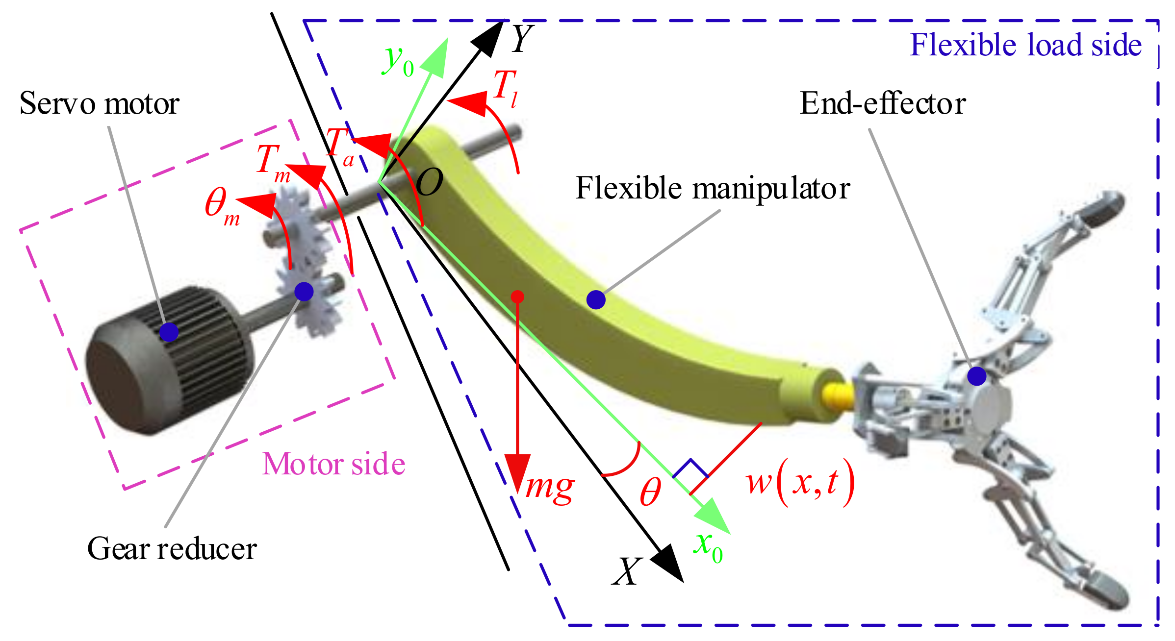
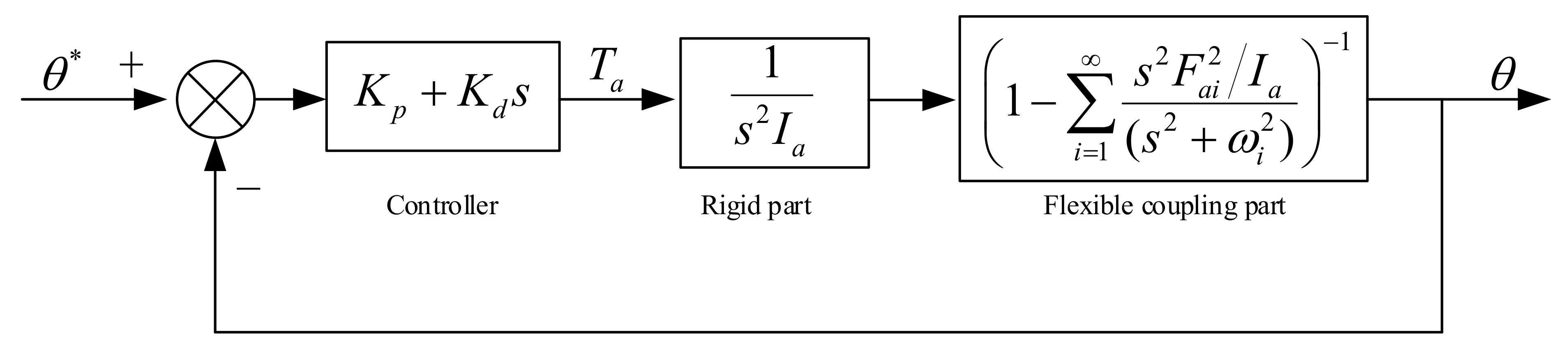
The servo system for flexible manipulators can be considered to be composed of a motor side and a flexible load side, as shown in Figure 1. The motor side contains a gear reducer that reduces the speed of the motor side. The flexibility of a flexible load is equivalent to the flexibility of a flexible manipulator. According to the literature [25,26], the flexible load can be equal to the Euler–Bernoulli flexible beam model.

where T_m, T_l, T_a represent the electromagnetic motor torque, the external torque of the load side, the input torque of the flexible load; w(x, t) represents the deformation of the flexible load; θ_m, θ represent the rotation angle of motor side, and the rotation angle of flexible load; XOY, x₀Oy₀ represent the static coordinate and the moving coordinate; mg represents the gravity.

If the torsional stiffness is ignored, the rotation angle of the motor side is equal to the rotation angle of the flexible load. Wherein, the relationship between T_m, T_l, and T_a is shown in Equation (1):

$$T_a=T_m-T_l.$$

(1)

According to the literature [27], the deformation of flexible loads is considered to be a two-dimensional function of the position of the load section x and time t. In the servo system’s modeling processes for flexible manipulators, the above model can be equivalent to the system that the cantilever beam rotates around the center. When the cantilever beam rotates, the transverse deformation of the flexible load is obvious. The longitudinal deformation occurs at the same time as the transverse deformation. According to the literature [28], the longitudinal deformation of the flexible load can be ignored since the longitudinal deformation is small. Therefore, the flexible load in the servo system for flexible manipulators is equivalent to an Euler–Bernoulli beam.

2.1. Description of Flexible Load-Deformation

According to the vibration theory of flexible beams, the deformation of the flexible load is described by the AMM. It is assumed that a flexible beam’s deformation is related to the modal function and the modal coordinate. The deformation of the flexible load is shown in Equation (2):

$$w\left(x,t\right)={\displaystyle \sum _{i=1}^{\infty }{\varphi }_i}\left(x\right){\delta }_i\left(t\right),$$

(2)

where ϕ_i(x), δ_i(t) represent the modal function and the modal coordinate.

The flexible manipulator’s external load is ignored, and the flexible load is equivalent to the flexible cantilever beam. Thus, the flexible load boundary conditions can be obtained, as shown in Equation (3):

$$\left\{\begin{array}{c}w\left(0,t\right)=0\\ \frac{\partial w\left(0,t\right)}{\partial x}=0\\ EI\frac{{\partial }^{2}w\left(l,t\right)}{\partial x^2}=0\\ EI\frac{{\partial }^{3}w\left(l,t\right)}{\partial x^3}=0\end{array}\right..$$

(3)

According to the vibration theory, the partial differential equation of the flexible load’s lateral vibration can be obtained, as shown in Equation (4):

$$\rho A\frac{{\partial }^{2}w\left(x,t\right)}{\partial t^2}+\frac{{\partial }^2}{\partial x^2}\left[EI\frac{{\partial }^{2}w\left(x,t\right)}{\partial x^2}\right]=0,$$

(4)

where ρ represents the volume density of flexible load; A represents the cross-section area of flexible load; EI represents the elastic modulus of flexible load.

Substituting Equation (2) into Equation (4), Equation (5) can be obtained:

$$\frac{{{\delta }^{″}}_i\left(t\right)}{{\delta }_i\left(t\right)}=-\frac{EI}{\rho A}\frac{{\varphi }_i{}^{\left(4\right)}\left(x\right)}{{\varphi }_i\left(x\right)}=-{\omega }_i^2,$$

(5)

where ω_i represents the modal frequency of the flexible load.

Equation (5) can be sorted out to get Equation (6):

$$EI{\varphi }_i{}^{\left(4\right)}\left(x\right)-{\omega }_i^2\rho A{\varphi }_i\left(x\right)=0.$$

(6)

Assume the expression of the modal function solution, as shown in Equation (7):

$${\varphi }_i\left(x\right)=e^{sx}.$$

(7)

According to Equations (6)–(9) can be obtained:

$${\beta }_i^4=\frac{{\omega }_i{}^2\rho A}{EI},$$

(8)

$$\frac{{\mathrm{d}}^4{\varphi }_i\left(x\right)}{\mathrm{d}x}={\beta }_i^4{\varphi }_i\left(x\right),$$

(9)

where β_i represents the characteristic root of the modal function. Its value is related to the flexible load length and boundary conditions. When the boundary conditions of the flexible load are consistent with the cantilever beam, the expression of the characteristic root value of the modal function is shown in Equation (10):

$$\cos {\beta }_{i}l\mathrm{ch}{\beta }_{i}l=-1.$$

(10)

According to Equation (8), the relationship between the modal frequency of the flexible load and the characteristic root of the modal function can be obtained, as shown in Equation (11):

$${\omega }_i=\sqrt{\frac{EI{\beta }_i{}^4}{\rho A}}.$$

(11)

Thus, the characteristic equation and characteristic root of the modal function can be obtained according to Equation (9), as shown in Equation (12):

$$\left\{\begin{array}{c}{s}^4-{\beta }^4=0\\ s_{1,2}=\pm \beta \\ s_{3,4}=\pm \mathrm{i}\beta \end{array}\right..$$

(12)

According to Equation (12), the solution of the modal function can be obtained, as shown in Equation (13).

$${\varphi }_i\left(x\right)=D_1\sin {\beta }_{i}x+D_2\cos {\beta }_{i}x+D_3\mathrm{sh}{\beta }_{i}x+D_4\mathrm{ch}{\beta }_{i}x$$

(13)

where D₁, D₂, D₃, and D₄ represent the coefficients that can be obtained by the boundary conditions.

According to literature [27], Equation (13) is sorted out to obtain Equation (14).

$${\varphi }_i\left(x\right)=\mathrm{ch}{\beta }_{i}x-\cos {\beta }_{i}x+{\varsigma }_i\left(\mathrm{sh}{\beta }_{i}x-\sin {\beta }_{i}x\right)$$

(14)

where the expression of ${\varsigma }_i$ can be obtained in Equation (15).

$${\varsigma }_i=-\frac{\mathrm{sh}{\beta }_{i}l-\sin {\beta }_{i}l}{\mathrm{ch}{\beta }_{i}l+\cos {\beta }_{i}l}$$

(15)

2.2. Modeling of the Flexible Manipulator Servo System

If the flexible manipulator moves in the horizontal plane, it does not need to consider gravity’s influence. In this case, the vector representation of any point on the flexible load is shown in Equation (16):

$$\left\{\begin{array}{l}{r}^{\mathrm{T}}=\left[X,Y\right]\\ X=x\cos \theta -w\left(x,t\right)\sin \theta \\ Y=x\sin \theta +w\left(x,t\right)\cos \theta \end{array}\right..$$

(16)

So, the kinetic energy of the flexible load is shown in Equation (17):

$$\begin{array}{l}T=\frac{1}{2}\rho A{\displaystyle {\int }_0^l{\dot{r}}^{\mathrm{T}}\dot{r}\mathrm{d}x}\\ =\frac{1}{2}\rho A{\displaystyle {\int }_0^l\left[\left(x^2+w{\left(x,t\right)}^2\right){\dot{\theta }}^2+{\left(\frac{\partial w\left(x,t\right)}{\partial t}\right)}^2+2x\frac{\partial w\left(x,t\right)}{\partial t}\dot{\theta }\right]\mathrm{d}x}\end{array}$$

(17)

The elastic potential energy of the flexible manipulator is shown in Equation (18):

$$V=\frac{1}{2}EI{\displaystyle {\int }_0^l\frac{{\partial }^{2}y\left(x,t\right)}{\partial x^2}}\mathrm{d}x.$$

(18)

According to the Lagrange Lagrange’s principle, Equation (19) can be obtained:

$$\frac{\mathrm{d}}{\mathrm{d}t}\left(\frac{\partial T}{\partial {\dot{q}}_i}\right)-\frac{\partial T}{\partial q_i}+\frac{\partial V}{\partial q_i}=Q_i,$$

(19)

where q₁, q₂ represent the rotation angle of flexible load and the modal coordinates; Q_i represents the generalized force.

Equation (19) can be obtained by Equation (20):

$$\left\{\begin{array}{l}\frac{\mathrm{d}}{\mathrm{d}t}\left(\frac{\partial T}{\partial \dot{\theta }}\right)-\frac{\partial T}{\partial \theta }+\frac{\partial V}{\partial \theta }=T_a\\ \frac{\mathrm{d}}{\mathrm{d}t}\left(\frac{\partial T}{\partial {\dot{\delta }}_i\left(t\right)}\right)-\frac{\partial T}{\partial {\delta }_i\left(t\right)}+\frac{\partial V}{\partial {\delta }_i\left(t\right)}=0\end{array}\right..$$

(20)

Equation (20) can be finally sorted into the form of Equation (21):

$$\left\{\begin{array}{c}\ddot{\theta }{\displaystyle {\int }_0^l\rho A{x}^2\mathrm{d}x+}\ddot{\theta }{\displaystyle \sum _{i=1}^{\infty }{\delta }_i{\left(t\right)}^2}+2\dot{\theta }{\displaystyle \sum _{i=1}^{\infty }{\delta }_i\left(t\right){\dot{\delta }}_i\left(t\right)}+{\displaystyle \sum _{i=1}^{\infty }{\ddot{\delta }}_i\left(t\right)}{\displaystyle {\int }_0^l\rho Ax{\varphi }_i\left(x\right)\mathrm{d}x}=T_a\\ {\displaystyle \sum _{i=1}^{\infty }{\ddot{\delta }}_i\left(t\right)}+\ddot{\theta }{\displaystyle \sum _{i=1}^{\infty }{\displaystyle {\int }_0^l\rho Ax{\varphi }_i\left(x\right)\mathrm{d}x}}-{\dot{\theta }}^2{\displaystyle \sum _{i=1}^{\infty }{\delta }_i\left(t\right)}+{\displaystyle \sum _{i=1}^{\infty }{\omega }^2{}_i{\delta }_i\left(t\right)}=0\end{array}\right..$$

(21)

Equations (22) and (23) are defined:

$$I_a=\rho A{\displaystyle {\int }_0^i{x}^2}\mathrm{d}x,$$

(22)

$$F_{ai}=\rho A{\displaystyle {\int }_0^{i}x{\varphi }_i\left(x\right)}\mathrm{d}x.$$

(23)

According to Equations (22) and (23), the servo system’s dynamic equation for flexible manipulators can be summarized in the form shown in Equation (24):

$$\left\{\begin{array}{c}{I}_a\ddot{\theta }+\ddot{\theta }{\displaystyle \sum _{i=1}^{\infty }{\delta }_i{\left(t\right)}^2}+2\dot{\theta }{\displaystyle \sum _{i=1}^{\infty }{\delta }_i\left(t\right){\dot{\delta }}_i\left(t\right)}+{\displaystyle \sum _{i=1}^{\infty }{\ddot{\delta }}_i\left(t\right)}{F}_{ai}=T_a\\ {\displaystyle \sum _{i=1}^{\infty }{\ddot{\delta }}_i\left(t\right)}+\ddot{\theta }{\displaystyle \sum _{i=1}^{\infty }{F}_{ai}}-{\dot{\theta }}^2{\displaystyle \sum _{i=1}^{\infty }{\delta }_i\left(t\right)}+{\displaystyle \sum _{i=1}^{\infty }{\omega }^2{}_i{\delta }_i\left(t\right)}=0\end{array}\right..$$

(24)

After removing the nonlinear terms, Equation (24) can be sorted out, as shown in Equation (25):

$$\left\{\begin{array}{c}{I}_a\ddot{\theta }+{\displaystyle \sum _{i=1}^{\infty }{\ddot{\delta }}_i\left(t\right)}{F}_{ai}=T_a\\ {\displaystyle \sum _{i=1}^{\infty }{\ddot{\delta }}_i\left(t\right)}+\ddot{\theta }{\displaystyle \sum _{i=1}^{\infty }{F}_{ai}}+{\displaystyle \sum _{i=1}^{\infty }{\omega }^2{}_i{\delta }_i\left(t\right)}=0\end{array}\right..$$

(25)

Equation (25) represents the servo system’s dynamic equation for flexible manipulators moving in the horizontal plane.

2.3. Modeling of Flexible Manipulator Servo System Considering the Gravity

If flexible manipulators move in the vertical plane, the influence of gravity needs to be considered. The flexible manipulator’s kinetic energy is still shown in Equation (17), but its potential energy can be approximately expressed, as shown in Equation (26):

$$V=\frac{1}{2}EI{\displaystyle {\int }_0^l\frac{{\partial }^{2}y\left(x,t\right)}{\partial x^2}}\mathrm{d}x+\frac{1}{2}gl\sin \theta {\displaystyle {\int }_0^l\rho A}\mathrm{d}x.$$

(26)

According to Lagrange’s principle, the dynamic Equation of the servo system for flexible manipulators considering the influence of gravity can be obtained, as shown in Equation (27):

$$\left\{\begin{array}{c}\ddot{\theta }{\displaystyle {\int }_0^l\rho A{x}^2\mathrm{d}x+}\ddot{\theta }{\displaystyle \sum _{i=1}^{\infty }{\delta }_i{\left(t\right)}^2}+2\dot{\theta }{\displaystyle \sum _{i=1}^{\infty }{\delta }_i\left(t\right){\dot{\delta }}_i\left(t\right)}+{\displaystyle \sum _{i=1}^{\infty }{\ddot{\delta }}_i\left(t\right)}{\displaystyle {\int }_0^l\rho Ax{\varphi }_i\left(x\right)\mathrm{d}x}+\frac{1}{2}gl\cos \theta {\displaystyle {\int }_0^l\rho A}\mathrm{d}x=T_a\\ {\displaystyle \sum _{i=1}^{\infty }{\ddot{\delta }}_i\left(t\right)}+\ddot{\theta }{\displaystyle \sum _{i=1}^{\infty }{\displaystyle {\int }_0^l\rho Ax{\varphi }_i\left(x\right)\mathrm{d}x}}-{\dot{\theta }}^2{\displaystyle \sum _{i=1}^{\infty }{\delta }_i\left(t\right)}+{\displaystyle \sum _{i=1}^{\infty }{\omega }^2{}_i{\delta }_i\left(t\right)}=0\end{array}\right.$$

(27)

Similarly, after removing the nonlinear term, the simplified dynamic equation can be obtained, as shown in Equation (28):

$$\left\{\begin{array}{c}\ddot{\theta }{\displaystyle {\int }_0^l\rho A{x}^2\mathrm{d}x+}{\displaystyle \sum _{i=1}^{\infty }{\ddot{\delta }}_i\left(t\right)}{\displaystyle {\int }_0^l\rho Ax{\varphi }_i\left(x\right)\mathrm{d}x}+\frac{1}{2}gl\cos \theta {\displaystyle {\int }_0^l\rho A}\mathrm{d}x=T_a\\ {\displaystyle \sum _{i=1}^{\infty }{\ddot{\delta }}_i\left(t\right)}+\ddot{\theta }{\displaystyle \sum _{i=1}^{\infty }{\displaystyle {\int }_0^l\rho Ax{\varphi }_i\left(x\right)\mathrm{d}x}}+{\displaystyle \sum _{i=1}^{\infty }{\omega }^2{}_i{\delta }_i\left(t\right)}=0\end{array}\right..$$

(28)

According to Equations (22) and (23), Equation (27) can be sorted into the form shown in Equation (29):

$$\left\{\begin{array}{c}{I}_a\ddot{\theta }+\ddot{\theta }{\displaystyle \sum _{i=1}^{\infty }{\delta }_i{\left(t\right)}^2}+2\dot{\theta }{\displaystyle \sum _{i=1}^{\infty }{\delta }_i\left(t\right){\dot{\delta }}_i\left(t\right)}+{\displaystyle \sum _{i=1}^{\infty }{\ddot{\delta }}_i\left(t\right)}{F}_{ai}+\frac{1}{2}gl\cos \theta {\displaystyle {\int }_0^l\rho A}\mathrm{d}x=T_a\\ {\displaystyle \sum _{i=1}^{\infty }{\ddot{\delta }}_i\left(t\right)}+\ddot{\theta }{\displaystyle \sum _{i=1}^{\infty }{F}_{ai}}-{\dot{\theta }}^2{\displaystyle \sum _{i=1}^{\infty }{\delta }_i\left(t\right)}+{\displaystyle \sum _{i=1}^{\infty }{\omega }^2{}_i{\delta }_i\left(t\right)}=0\end{array}\right..$$

(29)

According to Equation (29), Equation (30) can be obtained after removing the nonlinear term:

$$\left\{\begin{array}{c}{I}_a\ddot{\theta }+{\displaystyle \sum _{i=1}^{\infty }{\ddot{\delta }}_i\left(t\right)}{F}_{ai}+\frac{1}{2}gl\cos \theta {\displaystyle {\int }_0^l\rho A}\mathrm{d}x=T_a\\ {\displaystyle \sum _{i=1}^{\infty }{\ddot{\delta }}_i\left(t\right)}+\ddot{\theta }{\displaystyle \sum _{i=1}^{\infty }{F}_{ai}}+{\displaystyle \sum _{i=1}^{\infty }{\omega }^2{}_i{\delta }_i\left(t\right)}=0\end{array}\right..$$

(30)

Equation (29) represents the dynamic equation of the servo system for flexible manipulators considering gravity. Equation (31) represents the simplified form when nonlinear terms are not considered.

In order to study the influence of gravity on the input torque of flexible manipulators, a single link maneuver proposed by the literature [29] is also adopted. The relationship between the rotation angle and time is shown in Equation (31):

$$\ddot{\theta }\left(t\right)=\left\{\begin{array}{ll}\frac{{\dot{\theta }}_{\max }}{15}\left(1-\cos \frac{2\pi }{15}\left(t\right)\right)& 0\le t\le 15\\ 0& 15\le t\end{array}\right..$$

(31)

When gravity is taken into account, parameters such as the length and elastic modulus of flexible manipulators will affect the input torque. If only the first-order model is considered and the mass of the flexible manipulator is unchanged, the input torque can be obtained according to Equations (25) and (30), as shown in Figure 2.

According to Figure 2, the following conclusions can be drawn:

(1)

If the flexible manipulator moves on the vertical plane, gravity’s influence on the input torque is crucial and cannot be ignored.

(2)

The input torque under the influence of gravity increases as the flexible manipulator’s length increases.

(3)

Without considering the factor of gravity, the input torque is affected by the maximum rotation speed of the flexible manipulator, and the input torque increases with the increase of speed.

If the factor of gravity is considered, the input torque of the flexible manipulator is less affected by the maximum rotation speed. According to the above conclusion, when the flexible manipulator moves in the vertical plane, the influence of gravity should not be ignored.

3. Control Characteristics of Flexible Manipulator Servo System

3.1. Transfer Function of the Servo System

When the flexible manipulator moves in the horizontal plane, gravity’s influence does not need to be considered. Equation (25) can be used as the dynamic equation of the servo system for flexible manipulators. The dynamic equation shown in Equation (25) can be regarded as a single-input multiple-output system. The input torque of the flexible manipulator is taken as the input, and the rotation angle and the modal coordinates are taken as the output.

After the Laplace variation of Equation (25), Equation (32) can be obtained:

$$s^2\theta \left(I_a-{\displaystyle \sum _{i=1}^{\infty }\frac{s^2{F}_{ai}^2}{\left(s^2+{\omega }_i^2\right)}}\right)=T_a,$$

(32)

$$-I_a{\displaystyle \sum _{i=1}^{\infty }\frac{{\delta }_i\left(t\right)\left(s^2+{\omega }_i^2\right)}{F_{ai}}}+{\displaystyle \sum _{i=1}^{\infty }{\delta }_i\left(t\right)}{s}^2{F}_{ai}=T_a.$$

(33)

Only the first-order model, the servo system’s transfer function for flexible manipulators, can be obtained according to Equation (32), as shown in Equation (34):

$$\frac{\theta }{T_a}=\frac{1}{s^2\left(I_a-\frac{s^2{F}_{a1}^2}{\left(s^2+{\omega }_1^2\right)}\right)},$$

(34)

$$\frac{{\delta }_1\left(t\right)}{T_a}=\frac{F_{a1}}{s^2{F}_{a1}^2-I_a\left(s^2+{\omega }_1^2\right)}.$$

(35)

Equation (34) represents the transfer function from the input torque of flexible manipulators to the rotation angle. Equation (35) illustrates the transfer function from the input torque of flexible manipulators to the modal function.

If the effect of flexibility is not considered, the transfer function from the input torque of the manipulator to the rotation angle is shown in Equation (36):

$$G_1\left(s\right)=\frac{1}{s^2{I}_a}.$$

(36)

If we consider that flexible manipulators have a third-order mode, the transfer function from the input torque to the rotation angle is obtained, as shown in Equation (37):

$$G_2\left(s\right)=\frac{1}{s^2{I}_a}{\left(1-M\right)}^{-1},$$

(37)

where the expression of M is shown in Equation (38):

$$M=\frac{s^2{F}_{a1}^2/I_a}{(s^2+{\omega }_1^2)}+\frac{s^2{F}_{a2}^2/I_a}{(s^2+{\omega }_2^2)}+\frac{s^2{F}_{a3}^2/I_a}{(s^2+{\omega }_3^2)}.$$

(38)

According to Equation (37), the open-loop Bode diagram from the input torque to the flexible manipulator’s rotation angle can be obtained, as shown in Figure 3. According to Figure 3, the flexibility of the manipulator will cause oscillation frequency. When the oscillation frequency is close to the speed, it will cause more significant vibration. Therefore, it is necessary to consider the flexibility of the manipulator.

The length and the elastic modulus of the flexible manipulator will impact the oscillation frequency of the open-loop transfer function, as shown in Figure 4.

According to Figure 4, each mode’s oscillation frequency decreases with the increase of the manipulator’s length and increases with the growth of the elastic modulus. The manipulator will change the oscillation frequency in the telescopic movement due to the flexible factor, so it has strong robustness. This robustness will cause the motion error of the flexible manipulator and affect the accuracy. Therefore, the flexible factor should be considered for high precision manipulator:

By comparing Equations (36) and (37), the flexibility of manipulators is mainly reflected in the flexible coupling part, and its expression is shown in Equation (39). Compared with rigid manipulators, flexible manipulators have a flexible coupling part in the transfer function:

$$H\left(s\right)={\left(1-{\displaystyle \sum _{i=1}^{\infty }\frac{s^2{F}_{ai}^2/I_a}{(s^2+{\omega }_i^2)}}\right)}^{-1}.$$

(39)

3.2. Design of the PD Controller Based on Pole Placement Strategy

In the servo system for flexible manipulators, it is considered in the literature [30] that the control of the speed loop and current loop of the servo system has been completed. Therefore, the influence of the current loop and speed loop is ignored in this paper and considers position control. The position loop of the servo system adopts a PD control strategy, as shown in Figure 5.

where K_p, K_d represent the proportion coefficient and the differential coefficient.

According to Figure 5, the closed-loop transfer function of position control of the flexible manipulator can be obtained, as shown in Equation (40):

$$G_b\left(s\right)=\frac{\left(K_p+K_{d}s\right)\frac{1}{s^2{I}_a}{\left(1-{\displaystyle \sum _{i=1}^{\infty }\frac{s^2{F}_{ai}^2/I_a}{(s^2+{\omega }_i^2)}}\right)}^{-1}}{1+\left(K_p+K_{d}s\right)\frac{1}{s^2{I}_a}{\left(1-{\displaystyle \sum _{i=1}^{\infty }\frac{s^2{F}_{ai}^2/I_a}{(s^2+{\omega }_i^2)}}\right)}^{-1}}.$$

(40)

When only the first-mode is considered, the position control’s closed-loop transfer function is shown in Equation (41):

$$G_b\left(s\right)=\frac{K_d{s}^3+K_p{s}^2+K_d{\omega }_1^{2}s+K_p{\omega }_1^2}{\left(I_a-F_{a1}^2\right)s^4+K_d{s}^3+\left(K_p+I_a{\omega }_1^2\right)s^2+K_d{\omega }_1^{2}s+K_p{\omega }_1^2}.$$

(41)

According to the literature [21], the pole placement strategy is adopted to configure the closed-loop transfer function’s poles. The denominator polynomial of Equation (41) is written in the form shown in Equation (42):

$$\left\{\begin{array}{l}\left(I_a-F_{a1}^2\right)s^4+K_d{s}^3+\left(K_p+I_a{\omega }_1^2\right)s^2+K_d{\omega }_1^{2}s+K_p{\omega }_1^2=\left(I_a-F_{a1}^2\right)D\\ D=\left(s^2+2{\xi }_{a1}{\omega }_{a1}s+{\omega }_{a1}^2\right)\left(s^2+2{\xi }_{b1}{\omega }_{b1}s+{\omega }_{b1}^2\right)\end{array}\right.,$$

(42)

where ${\xi }_{a1}$, ${\xi }_{b1}$ denote the damping coefficients of the poles; ${\omega }_{a1}$, ${\omega }_{b1}$ denote the natural frequency coefficients of the poles.

According to Equation (42), Equation (43) can be obtained:

$$\left(s^2+2{\xi }_{a1}{\omega }_{a1}s+{\omega }_{a1}^2\right)\left(s^2+2{\xi }_{b1}{\omega }_{b1}s+{\omega }_{b1}^2\right)=s^4+\frac{K_d}{\left(I_a-F_{a1}^2\right)}{s}^3+\frac{\left(K_p+I_a{\omega }_1^2\right)}{\left(I_a-F_{a1}^2\right)}{s}^2+\frac{K_d{\omega }_1^2}{\left(I_a-F_{a1}^2\right)}s+\frac{K_p{\omega }_1^2}{\left(I_a-F_{a1}^2\right)}.$$

(43)

Therefore, Equations (44)–(47) can be obtained:

$$2{\xi }_{a1}{\omega }_{a1}+2{\xi }_{b1}{\omega }_{b1}=\frac{K_d}{\left(I_a-F_{a1}^2\right)},$$

(44)

$${\omega }_{a1}^2+{\omega }_{b1}^2+4{\xi }_{a1}{\xi }_{b1}{\omega }_{a1}{\omega }_{b1}=\frac{\left(K_p+I_a{\omega }_1^2\right)}{\left(I_a-F_{a1}^2\right)},$$

(45)

$$2{\xi }_{a1}{\omega }_{a1}{\omega }_{b1}^2+2{\xi }_{b1}{\omega }_{b1}{\omega }_{a1}^2=\frac{K_d{\omega }_1^2}{\left(I_a-F_{a1}^2\right)},$$

(46)

$${\omega }_{a1}^2{\omega }_{b1}^2=\frac{K_p{\omega }_1^2}{\left(I_a-F_{a1}^2\right)}.$$

(47)

The determination of PD controller parameters is the core of using the PD control method to control the servo system for flexible manipulators. According to Equations (44)–(47), pole placement strategy is used to calculate controller parameters. The PD controller parameters are shown in Equations (48) and (49):

$$K_p=\frac{{\omega }_{a1}^2{\omega }_{b1}^2\left(I_a-F_{a1}^2\right)}{{\omega }_1^2},$$

(48)

$$K_d=\left(2{\xi }_{a1}{\omega }_{a1}+2{\xi }_{b1}{\omega }_{b1}\right)\left(I_a-F_{a1}^2\right).$$

(49)

In this paper, the pole placement strategy with the same damping coefficient is used to determine the controller parameters. That means that the closed-loop transfer function of the system has the same damping coefficient. Substitute ${\xi }_{a1}={\xi }_{b1}={\xi }_1$ into the Equations (44)–(47), and Equations (50) and (51) can be obtained after sorting out:

$$2{\xi }_1\left({\omega }_{a1}+{\omega }_{b1}\right)=\frac{K_d}{\left(I_a-F_{a1}^2\right)},$$

(50)

$${\omega }_{a1}^2+{\omega }_{b1}^2+4{\xi }_1{}^2{\omega }_{a1}{\omega }_{b1}=\frac{\left(K_p+I_a{\omega }_1^2\right)}{\left(I_a-F_{a1}^2\right)}.$$

(51)

According to Equations (50) and (51), Equations (52) and (53) can be obtained:

$$\left(\frac{{\omega }_{a1}^2+{\omega }_{b1}^2}{{\omega }_{a1}{\omega }_{b1}}\right)+4{\xi }_1{}^2=\frac{\left(I_a-F_{a1}^2+I_a\right)}{\left(I_a-F_{a1}^2\right)}=\frac{\left(2I_a-2F_{a1}^2+F_{a1}^2\right)}{\left(I_a-F_{a1}^2\right)}=\frac{F_{a1}^2}{I_a-F_{a1}^2}+2,$$

(52)

$${\omega }_1^2={\omega }_{a1}{\omega }_{b1}^{}.$$

(53)

According to Equations (52) and (53), Equations (54) and (55) can be obtained:

$${\omega }_{a1}=\frac{\sqrt{\frac{F_{a1}^2}{I_a-F_{a1}^2}-4{\xi }_1^2+4}-\sqrt{\frac{F_{a1}^2}{I_a-F_{a1}^2}-4{\xi }_1^2}}{2}{\omega }_1,$$

(54)

$${\omega }_{b1}=\frac{\sqrt{\frac{F_{a1}^2}{I_a-F_{a1}^2}-4{\xi }_1^2+4}+\sqrt{\frac{F_{a1}^2}{I_a-F_{a1}^2}-4{\xi }_1^2}}{2}{\omega }_1.$$

(55)

According to Equations (54) and (55), the control parameters can be obtained as shown in Equations (56) and (57):

$$K_d=2{\xi }_1\left(I_a-F_{a1}^2\right)\sqrt{\frac{F_{a1}^2}{I_a-F_{a1}^2}-4{\xi }_1^2+4}{\omega }_1,$$

(56)

$$K_p=\left(I_a-F_{a1}^2\right){\omega }_1^2.$$

(57)

According to the control parameters, the servo system’s closed-loop transfer function for flexible manipulators can be obtained, as shown in Equation (58):

$$G_b\left(s\right)=\frac{\left(2{\xi }_1\sqrt{\frac{F_{a1}^2}{I_a-F_{a1}^2}-4{\xi }_1^2+4}\right){\omega }_1{s}^3+{\omega }_1^2{s}^2+\left(2{\xi }_1\sqrt{\frac{F_{a1}^2}{I_a-F_{a1}^2}-4{\xi }_1^2+4}\right){\omega }_1^{3}s+{\omega }_1^4}{s^4+\left(2{\xi }_1\sqrt{\frac{F_{a1}^2}{I_a-F_{a1}^2}-4{\xi }_1^2+4}\right){\omega }_1{s}^3+\left({\omega }_1^2+\frac{I_a{\omega }_1^2}{I_a-F_{a1}^2}\right)s^2+\left(2{\xi }_1\sqrt{\frac{F_{a1}^2}{I_a-F_{a1}^2}-4{\xi }_1^2+4}\right){\omega }_1^{3}s+{\omega }_1^4}.$$

(58)

The parameters of the PD controller can be adjusted indirectly by adjusting the damping coefficient of the poles. The controller parameters can be calculated according to Equations (56) and (57) to achieve a stable and fast output of the system.

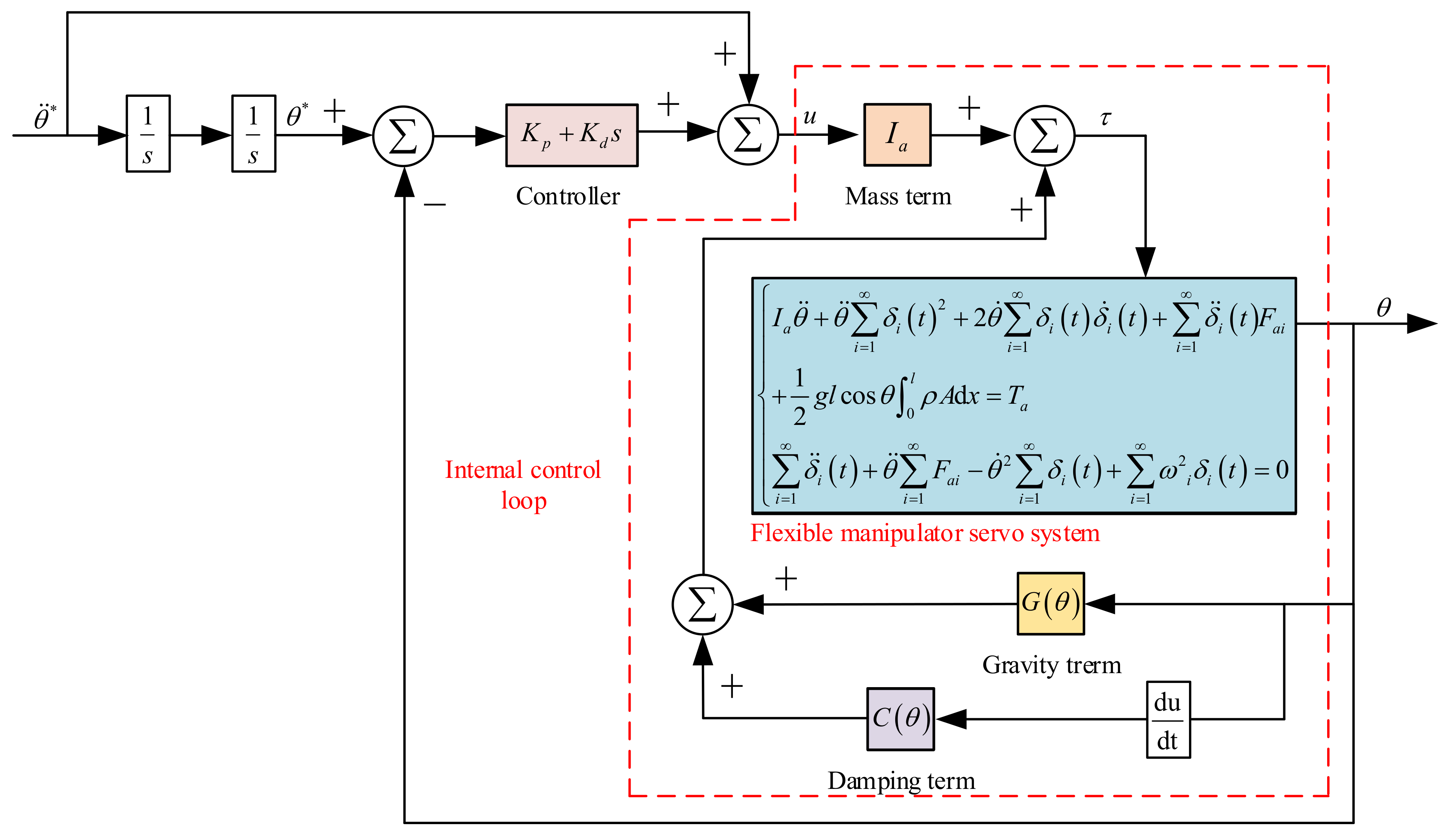
4. Control Method of Flexible Manipulators Based on RBF Neural Network

When flexible manipulators move in a vertical plane, the gravity factor cannot be ignored. Due to the nonlinear factors caused by gravity and flexibility, the difficulty of flexible manipulators control is increased. Therefore, the nonlinear control method of flexible manipulators is adopted in this paper. Nonlinear compensation is introduced into the inner control loop to offset the influence of gravity nonlinear term. The nonlinear part caused by flexibility is regarded as the disturbance term, which increases uncertain items in the system. During the compound motion of flexible manipulators, the parameters such as inertia have significant time-varying characteristics. Therefore, the servo drive system for flexible manipulators has strong robustness, bringing difficulty to precise control. In order to solve the uncertain items caused by flexibility and time-varying characteristics of the parameters, the RBF neural network is used to approximate the uncertain items. The accurate input torque of flexible manipulators can be obtained by introducing an internal control loop with nonlinear terms and identify the system’s uncertain items with the RBF neural network. Then, the angle error and the vibration amplitude of flexible manipulators are reduced.

According to Equation (30), the servo system’s dynamic equation for flexible manipulators considering gravity can be obtained. Equation (30) is simplified into a general form, as shown in Equation (59):

$$\left\{\begin{array}{l}{I}_a\ddot{\theta }+C\left(\theta \right)\dot{\theta }+G\left(\theta \right)=\tau +d\\ G\left(\theta \right)=\frac{1}{2}gl\cos \theta {\displaystyle {\int }_0^l\rho A}\mathrm{d}x\\ \tau =T_a\\ d=-\left(2\dot{\theta }{\displaystyle \sum _{i=1}^{\infty }{\delta }_i\left(t\right){\dot{\delta }}_i\left(t\right)}+{\displaystyle \sum _{i=1}^{\infty }{\ddot{\delta }}_i\left(t\right)}{F}_{ai}\right)\end{array}\right.,$$

(59)

where C(θ), G(θ), represent the damping coefficient and the gravity item respectively. If the damping effect is ignored, then C(θ) = 0. The symbol τ and d represent the input torque of the flexible load and the disturbance term respectively.

4.1. Internal Control Loop with Nonlinear Compensation Term

According to Equation (30) and Figure 2, the gravity factor cannot be ignored during the movement of flexible manipulators in a vertical plane. When calculating the input torque of flexible manipulators, whether the gravity factor is considered or not has a significant difference in the calculation results. In this paper, the inner control loop is added based on the PD control strategy that controls the servo system’s position loop for flexible manipulators. The parameters of the PD controller are determined by pole placement strategy. A nonlinear gravity compensation term is added to the internal control loop. The input torque generated by the system can compensate for the influence of gravity in real-time. The schematic diagram of the servo system’s internal control loop for flexible manipulators with nonlinear compensation is shown in Figure 6.

It is assumed that the uncertain items are not considered in the servo system for flexible manipulators. According to Figure 6, the control law of the PD control strategy with the inner control loop can be obtained, as shown in Equation (60):

$$\left\{\begin{array}{l}\tau =I_{a}u+C\left(\theta \right)\dot{\theta }+G\left(\theta \right)\\ u={\ddot{\theta }}^{*}-K_d\dot{e}-K_{p}e\\ e=\theta -{\theta }^{*}\\ \dot{e}=\dot{\theta }-{\dot{\theta }}^{*}\\ \ddot{e}=\ddot{\theta }-{\ddot{\theta }}^{*}\end{array}\right..$$

(60)

Thus, the closed-loop system equation under this control strategy can be obtained, as shown in Equation (61):

$$\ddot{e}+K_d\dot{e}+K_{p}e=0.$$

(61)

4.2. Control Law Considering the Uncertain Items

Due to the time-varying characteristics of parameters and flexible nonlinear terms in the servo system for flexible manipulators, proper system parameters cannot be obtained. Therefore, only nominal models can be established. For the nominal system, the control law is shown in Equation (62):

$$\tau ={\widehat{I}}_a\left({\ddot{\theta }}^{*}-K_d\dot{e}-K_{p}e\right)+\widehat{C}\left(\theta \right)\dot{\theta }+\widehat{G}\left(\theta \right),$$

(62)

where ${\widehat{I}}_a$, $\widehat{C}\left(\theta \right)$, $\widehat{G}\left(\theta \right)$ represent the nominal coefficients of the inertia, the damping coefficient, and the gravity item respectively; ${\theta }^{*}$ represents the desired angular trajectory.

By substituting the control law of the nominal system into Equation (59), Equation (63) can be obtained:

$${\widehat{I}}_a\left({\ddot{\theta }}^{*}-K_d\dot{e}-K_{p}e\right)+\widehat{C}\left(\theta \right)\dot{\theta }+\widehat{G}\left(\theta \right)+d=I_a\ddot{\theta }+C\left(\theta \right)\dot{\theta }+G\left(\theta \right).$$

(63)

After simplification of Equation (63), Equation (64) can be obtained:

$${\widehat{I}}_a\left[\left(\ddot{\theta }-{\ddot{\theta }}^{*}\right)+K_d\dot{e}+K_{p}e\right]=\left({\widehat{I}}_a-I_a\right)\ddot{\theta }+\left(\widehat{C}\left(\theta \right)-C\left(\theta \right)\right)\dot{\theta }+\left(\widehat{G}\left(\theta \right)-G\left(\theta \right)\right)+d.$$

(64)

Equation (64) shows the closed-loop system equation with deterministic considerations, as shown in Equation (65):

$$\left\{\begin{array}{l}\ddot{e}+K_d\dot{e}+K_{p}e={\widehat{I}}_a{}^{-1}\left(\Delta I_a\ddot{\theta }+\Delta C\left(\theta \right)\dot{\theta }+\Delta G\left(\theta \right)+d\right)\\ \Delta I_a={\widehat{I}}_a-I_a\\ \Delta C\left(\theta \right)=\widehat{C}\left(\theta \right)-C\left(\theta \right)\\ \Delta G\left(\theta \right)=\widehat{G}\left(\theta \right)-G\left(\theta \right)\end{array}\right.,$$

(65)

where ΔI_a, ΔC(θ), and ΔG(θ) represent the difference between nominal coefficients and real coefficients of the inertia, the damping coefficient, and the gravity item, respectively.

According to Equation (65), the uncertain items can be obtained, and its expression is shown in Equation (66):

$$f={\widehat{I}}_a{}^{-1}\left(\Delta I_a\ddot{\theta }+\Delta C\left(\theta \right)\dot{\theta }+\Delta G\left(\theta \right)+d\right).$$

(66)

Based on Equations (65) and (66), the error state equation of the system can be obtained under the condition of considering system uncertain items, as shown in Equation (67):

$$\ddot{e}=-K_{p}e-K_d\dot{e}+f.$$

(67)

Equation (67) can be written as shown in Equation (68):

$$\left\{\begin{array}{l}\dot{\mathit{x}}=A\mathit{x}+Bf\\ \mathit{x}={\left[\begin{array}{cc}e& \dot{e}\end{array}\right]}^{\mathrm{T}}\\ A=\left[\begin{array}{cc}0& 1\\ -K_p& -K_d\end{array}\right]\\ B={\left[\begin{array}{cc}0& 1\end{array}\right]}^{\mathrm{T}}\end{array}\right..$$

(68)

Assuming that the uncertain items are known, the control law of servo system for flexible manipulators is shown in Equation (69):

$$\tau =\widehat{D}\left(\theta \right)\left({\ddot{\theta }}^{*}-K_d\dot{e}-K_{p}e-f\right)+\widehat{C}\left(\theta \right)\dot{\theta }+\widehat{G}\left(\theta \right).$$

(69)

By substituting Equation (68) into Equation (59), the stable closed-loop system equation can be obtained, as shown in Equation (61).

Because flexible manipulators’ parameters are time-varying and the flexible item is nonlinear, the uncertain items cannot be obtained. Therefore, it is necessary to identify the uncertain items to ensure the precise input torque of flexible manipulators.

4.3. RBF Neural Network to Identify the Uncertain Items of the Model

In this paper, the RBF neural network is used to approximate the uncertain items of the servo system for flexible manipulators. The result after approximation by the neural network replaces the real uncertain items of the system.

In the RBF neural network, the most common activation function is Gaussian [31]. The Gaussian activation function has the following advantages:

(1)

The representation is simple. It does not add too much complexity to multi-variable input.

(2)

Radial symmetry.

(3)

The smoothness is good, and the derivative of any order exists.

In this paper, the Gaussian function is used as the activation function of the RBF neural network, and the output of the ith node of the neural network can be expressed by Equation (70):

$$\left\{\begin{array}{l}{u}_i\left(\mathit{x}\right)=\exp \left(\frac{{\left(\mathit{x}-{\mathit{c}}_{\mathit{i}}\right)}^{\mathrm{T}}\left(\mathit{x}-{\mathit{c}}_{\mathit{i}}\right)}{2{\sigma }_i^2}\right),i=1,2,\cdots ,n\\ \mathit{x}={\left[x_1 x_2 \cdots x_n\right]}^{\mathrm{T}}={\left[\left(e_1,{\dot{e}}_1\right) \left(e_2,{\dot{e}}_2\right) \cdots \left(e_n,{\dot{e}}_n\right)\right]}^{\mathrm{T}}\end{array}\right.,$$

(70)

where u_i (x) represents the output of the ith hidden node; σ_i represents the normalizing constant of the ith hidden node; n represents the number of nodes of the hidden layer; c_i represents the center vector of the ith hidden node of the Gaussian function; x represents the input samples.

The hidden layer of the RBF neural network to the output layer realizes linear mapping. The result of the output layer is shown in Equation (71):

$$\left\{\begin{array}{l}{y}_k={\mathit{w}}_{\mathit{k}}\mathit{u}={\displaystyle \sum _{i=1}^n{w}_{ki}}{u}_i\\ y_k=\widehat{f}\end{array}\right.,$$

(71)

where y_k represents the output of the kth node of the output layer; w_k represents the weight coefficient vector; w_ki represents weight coefficient. In this paper, there is only one output node, which represents the system uncertain items.

According to Equations (70) and (71), it can be known that the system uncertain items are a function of the input samples and the weight coefficient vector. Use the $\widehat{f}\left(\mathit{x},{\mathit{w}}_{\mathit{k}}\right)$ to represent the uncertain items of the system identified by the neural network. The real uncertain items are a function of the state vector of the error. Use the f(x) to represent the uncertain items of the real system.

This article makes the following assumptions:

(1)

The RBF neural network output continuously.

(2)

The output of the RBF neural network approximates a continuous function f(x), and there is a very small positive number ε₀ that satisfies the condition of Equation (72):

$$\max ‖\widehat{f}\left(\mathit{x},{\mathit{w}}_k^{*}\right)-f\left(\mathit{x}\right)‖\le {\epsilon }_0.$$

(72)

According to the above assumptions, the error state-space equation shown in Equation (68) can be written into the form shown in Equation (73):

$$\dot{\mathit{x}}=\mathit{A}\mathit{x}+\mathit{B}\left\{\widehat{f}\left(\mathit{x},{\mathit{w}}_k^{*}\right)+\left[f\left(\mathit{x}\right)-\widehat{f}\left(\mathit{x},{\mathit{w}}_k^{*}\right)\right]\right\},$$

(73)

where ${\mathit{w}}_k^{*}$ represents the neural network weight coefficient vector for the optimal identification of system uncertain items. Its expression is shown in Equation (74):

$${\mathit{w}}_k^{*}=\arg \left(\min \left\{\sup ‖f\left(\mathit{x}\right)-\widehat{f}\left(\mathit{x},{\mathit{w}}_k^{}\right)‖\right\}\right).$$

(74)

This paper uses the η to represent the neural network error, and its expression is shown in Equation (75):

$$\mathit{\eta }=f\left(\mathit{x}\right)-\widehat{f}\left(\mathit{x},{\mathit{w}}_k^{*}\right).$$

(75)

According to Equation (75), the error state space-equation is written in the form shown in Equation (76):

$$\dot{\mathit{x}}=\mathit{A}\mathit{x}+\mathit{B}\left\{\widehat{f}\left(\mathit{x},{\mathit{w}}_k^{*}\right)+\mathit{\eta }\right\}.$$

(76)

After training, the neural network’s weight coefficient vector becomes ${\mathit{w}}_k^{*}$, then the output value of the neural network at this time is shown in Equation (77):

$$\widehat{f}\left(\mathit{x},{\mathit{w}}_k^{*}\right)={\displaystyle \sum _{i=1}^n{w}_{ki}^{*}}{u}_i.$$

(77)

According to Equation (66), the error state-space equation is written in the form shown in Equation (78):

$$\dot{\mathit{x}}=\mathit{A}\mathit{x}+\mathit{B}\left\{{\displaystyle \sum _{i=1}^n{w}_{ki}^{*}}{u}_i+\mathit{\eta }\right\}.$$

(78)

After applying the RBF neural network to identify the uncertain items, the servo drive system’s control law for flexible manipulators is shown in Equation (79):

$$\tau ={\widehat{I}}_a\left({\ddot{\theta }}^{*}-K_d\dot{e}-K_{p}e-\widehat{f}\left(\mathit{x},{\widehat{\mathit{w}}}_k^{}\right)\right)+\widehat{C}\left(\theta \right)\dot{\theta }+\widehat{G}\left(\theta \right),$$

(79)

where ${\widehat{\mathit{w}}}_k^{}$ represents the estimated value of ${\mathit{w}}_k^{*}$.

After using the RBF neural network to identify the uncertain items, the control loop’s schematic diagram is shown in Figure 7.

4.4. Proof of Stability

The RBF neural network is used to approach the uncertain items of the servo system for flexible manipulators. The control law is obtained, as shown in Equation (79). By substituting Equation (79) into Equation (59), Equation (80) can be obtained:

$$\ddot{e}+K_d\dot{e}+K_{p}e=\widehat{f}\left(\mathit{x},{\mathit{w}}_k^{*}\right)+f\left(\mathit{x}\right)-\widehat{f}\left(\mathit{x},{\mathit{w}}_k^{*}\right)-\widehat{f}\left(\mathit{x},{\widehat{\mathit{w}}}_k^{}\right).$$

(80)

According to Equation (80), Equation (81) can be obtained:

$$\ddot{e}+K_d\dot{e}+K_{p}e=\widehat{f}\left(\mathit{x},{\mathit{w}}_k^{*}\right)-\widehat{f}\left(\mathit{x},{\widehat{\mathit{w}}}_k^{}\right)+\mathit{\eta }={\displaystyle \sum _{i=1}^n{w}_{ki}^{*}}{u}_i-{\displaystyle \sum _{i=1}^n{\widehat{w}}_{ki}^{}}{u}_i+\mathit{\eta }.$$

(81)

Equation (82) is established:

$${\tilde{w}}_{ki}^{}={\widehat{w}}_{ki}^{}-w_{ki}^{*}.$$

(82)

Then, Equation (81) is written as shown in Equation (83):

$$\ddot{e}+K_d\dot{e}+K_{p}e=\widehat{f}\left(\mathit{x},{\mathit{w}}_k^{*}\right)-\widehat{f}\left(\mathit{x},{\widehat{\mathit{w}}}_k^{}\right)+\mathit{\eta }=-{\displaystyle \sum _{i=1}^n{\tilde{w}}_{ki}^{}}{u}_i+\mathit{\eta }.$$

(83)

According to Equation (83), the error state-space equation can be obtained, as shown in Equation (84):

$$\dot{\mathit{x}}=\mathit{A}\mathit{x}+\mathit{B}\left\{-{\displaystyle \sum _{i=1}^n{\tilde{w}}_{ki}^{}}{u}_i+\mathit{\eta }\right\}=\mathit{A}\mathit{x}+\mathit{B}\left\{-{\tilde{\mathit{w}}}_{\mathit{k}}^{}{}^{\mathrm{T}}\mathit{u}\left(x\right)+\mathit{\eta }\right\},$$

(84)

where ${\tilde{\mathit{w}}}_k^{}$ represents the difference between the optimal weight coefficients vector of neural network after training and the estimated weight coefficients vector; u(x) represents the output vector of the hidden node of the neural network.

The Lyapunov function is defined as Equation (85):

$$\mathrm{V}=\frac{1}{2}{\mathit{x}}^{\mathrm{T}}\mathit{P}\mathit{x}+\frac{1}{2\gamma }{‖{\tilde{\mathit{w}}}_{\mathit{k}}^{}‖}^2,$$

(85)

where γ is a positive number; P is a positive definite matrix and satisfies the Lyapunov function, as shown in Equation (86):

$$\mathit{P}\mathit{A}+{\mathit{A}}^{\mathrm{T}}\mathit{P}=-\mathit{Q},$$

(86)

where Q is a positive definite matrix.

According to Equation (85), Equation (87) can be obtained:

$$\left\{\begin{array}{l}\mathrm{V}={\mathrm{V}}_1+{\mathrm{V}}_2\\ {\mathrm{V}}_1=\frac{1}{2}{\mathit{x}}^{\mathrm{T}}\mathit{P}\mathit{x}\\ {\mathrm{V}}_2=\frac{1}{2\gamma }{‖{\tilde{\mathit{w}}}_{\mathit{k}}^{}‖}^2\end{array}\right..$$

(87)

According to Equation (87), Equation (88) can be obtained:

$$\left\{\begin{array}{l}{\dot{\mathrm{V}}}_1=\frac{1}{2}{\dot{\mathit{x}}}^{\mathrm{T}}\mathit{P}\mathit{x}+\frac{1}{2}{\mathit{x}}^{\mathrm{T}}\mathit{P}\dot{\mathit{x}}=\frac{1}{2}\left({\mathit{x}}^{\mathrm{T}}{\mathit{A}}^{\mathrm{T}}+{\mathit{M}}^{\mathrm{T}}\right)\mathit{P}\mathit{x}+\frac{1}{2}{\mathit{x}}^{\mathrm{T}}\mathit{P}\left(\mathit{A}\mathit{x}+\mathit{M}\right)\\ \hspace{1em}=\frac{1}{2}{\mathit{x}}^{\mathrm{T}}\left({\mathit{A}}^{\mathrm{T}}\mathit{P}+\mathit{P}\mathit{A}\right)\mathit{x}+\frac{1}{2}{\mathit{M}}^{\mathrm{T}}\mathit{P}\mathit{x}+\frac{1}{2}{\mathit{x}}^{\mathrm{T}}\mathit{P}\mathit{M}\\ \hspace{1em}=-\frac{1}{2}{\mathit{x}}^{\mathrm{T}}\mathit{Q}\mathit{x}+\frac{1}{2}\left({\mathit{M}}^{\mathrm{T}}\mathit{P}\mathit{x}+{\mathit{x}}^{\mathrm{T}}\mathit{P}\mathit{M}\right)=-\frac{1}{2}{\mathit{x}}^{\mathrm{T}}\mathit{Q}\mathit{x}+{\mathit{x}}^{\mathrm{T}}\mathit{P}\mathit{M}\\ {\dot{\mathrm{V}}}_2=\frac{1}{\gamma }{\tilde{\mathit{w}}}_{\mathit{k}}^{}{}^{\mathrm{T}}{\dot{\tilde{\mathit{w}}}}_{\mathit{k}}^{}\\ {\dot{\mathrm{V}}}_{}={\dot{\mathrm{V}}}_1+{\dot{\mathrm{V}}}_2=-\frac{1}{2}{\mathit{x}}^{\mathrm{T}}\mathit{Q}\mathit{x}+{\mathit{x}}^{\mathrm{T}}\mathit{P}\mathit{M}+\frac{1}{\gamma }{\tilde{\mathit{w}}}_{\mathit{k}}^{}{}^{\mathrm{T}}{\dot{\tilde{\mathit{w}}}}_{\mathit{k}}^{}\end{array}\right..$$

(88)

In Equation (88), the expression of M is shown in Equation (89):

$$\mathit{M}=\mathit{B}\left\{-{\tilde{\mathit{w}}}_{\mathit{k}}^{}{}^{\mathrm{T}}\mathit{u}\left(x\right)+\mathit{\eta }\right\}.$$

(89)

So, Equation (90) can be obtained:

$$\dot{\mathrm{V}}=-\frac{1}{2}{\mathit{x}}^{\mathrm{T}}\mathit{Q}\mathit{x}+{\mathit{x}}^{\mathrm{T}}\mathit{P}\mathit{B}\left\{-{\tilde{\mathit{w}}}_{\mathit{k}}^{}{}^{\mathrm{T}}\mathit{u}\left(x\right)+\mathit{\eta }\right\}=-\frac{1}{2}{\mathit{x}}^{\mathrm{T}}\mathit{Q}\mathit{x}+{\mathit{x}}^{\mathrm{T}}\mathit{P}\mathit{B}\mathit{\eta }+\frac{1}{\gamma }{\tilde{\mathit{w}}}_{\mathit{k}}^{}{}^{\mathrm{T}}\left(-\gamma {\mathit{x}}^{\mathrm{T}}\mathit{P}\mathit{B}\mathit{u}\left(x\right)+{\dot{\tilde{\mathit{w}}}}_{\mathit{k}}^{}\right).$$

(90)

The adaptive law of the RBF neural network is shown in Equation (91):

$${\dot{\tilde{\mathit{w}}}}_k^{}=\gamma {\mathit{x}}^{\mathrm{T}}\mathit{P}\mathit{B}\mathit{u}\left(x\right).$$

(91)

By substituting Equation (91) into Equation (90), the derivative of the Lyapunov function can be obtained as shown in Equation (92):

$$\dot{\mathrm{V}}=-\frac{1}{2}{\mathit{x}}^{\mathrm{T}}\mathit{Q}\mathit{x}+{\mathit{x}}^{\mathrm{T}}\mathit{P}\mathit{B}\mathit{\eta }.$$

(92)

By choosing the matrix Q and the small error η, the Lyapunov function’s derivative can be less than 0. Under this condition, the servo system for flexible manipulators is stable.

5. Numerical Simulation Analysis and Experiment

In this paper, the control method combining the pole placement strategy and the RBF neural network is used to improve the motion accuracy of flexible manipulators. The PD controller parameters are optimized according to the pole placement strategy. Besides, the RBF neural network is used to identify the uncertain items of flexible manipulators. So, the input torque of flexible manipulators is more accurate. Therefore, the precision of the rotation angle of flexible manipulators is improved. In order to verify the effectiveness of the proposed control strategy, numerical simulation and physical control experiments of flexible manipulators are carried out in this paper. Firstly, the influence of the physical parameters of flexible manipulators on the input torque and resonance frequency are analyzed by numerical simulation experiments. Next, the influence of the damping coefficient of poles on the rotation angle is analyzed. Finally, the numerical simulation experiment and experiment of the servo control for flexible manipulator are carried out.

5.1. The influence of Physical Parameters of the Manipulator

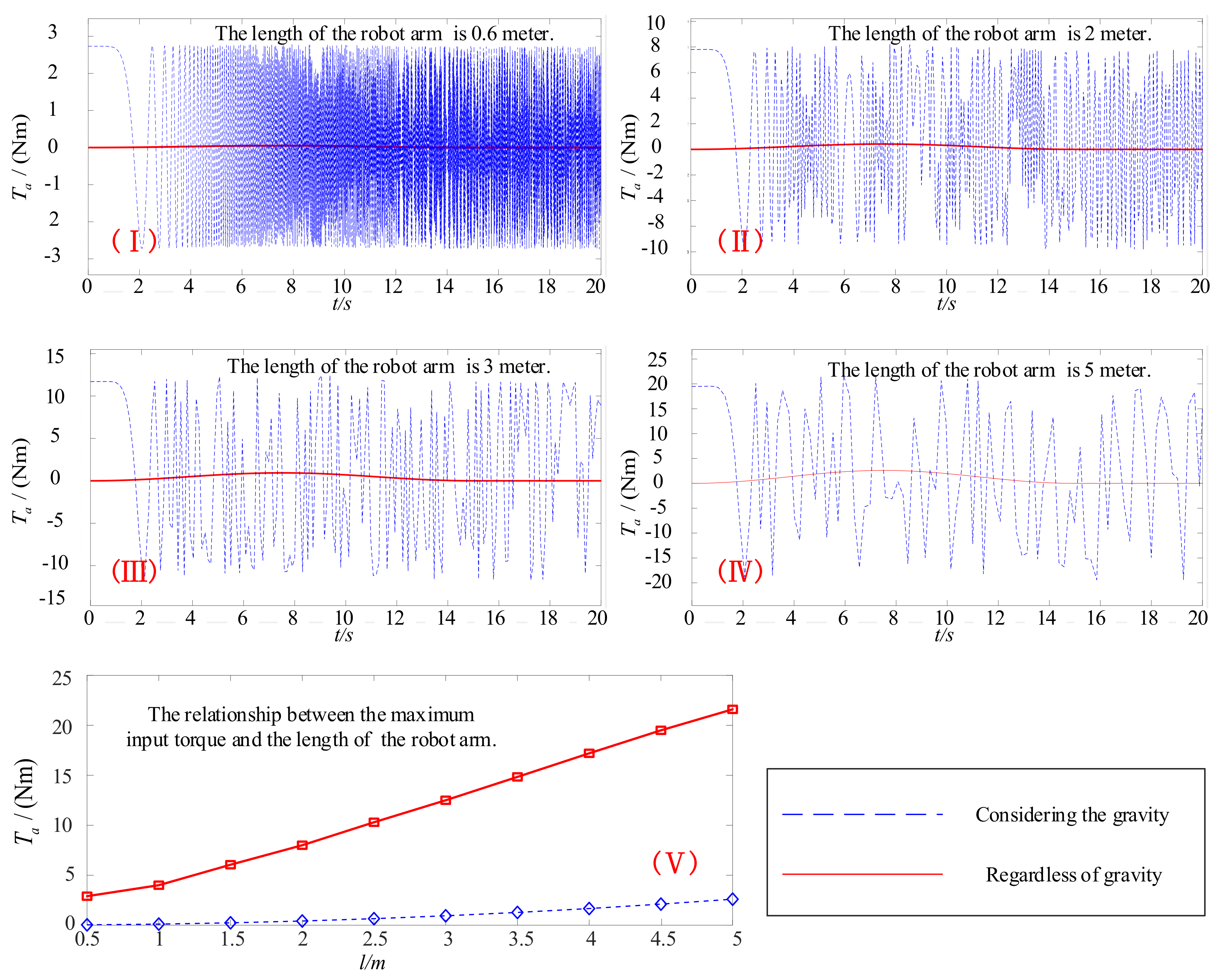
The length and elastic modulus of flexible manipulators will affect the servo system’s input torque and resonance frequency. Among them, the value of the input torque is closely related to the length of the manipulator. Besides, the input torque is closely associated with the gravity term. In this paper, according to Equation (25), Equation (30), and Equation (31), the relationship between input torque and time under different manipulators’ lengths is respectively calculated in two conditions, as shown in Figure 8. One of the cases ignores the gravitational factor, and the other case considers the gravitational factor.

According to Figure 8, the servo system’s maximum input torque increases with the increase of the length of manipulators. Among them, the gravity factor has a more significant influence on the maximum input torque. Relative to the manipulator’s length, the gravity factor is the dominant factor for the maximum input torque. Therefore, the internal control loop with nonlinear term compensation can effectively reduce the maximum input torque. Moreover, this control strategy can effectively reduce the fluctuation degree of the servo system’s output torque.

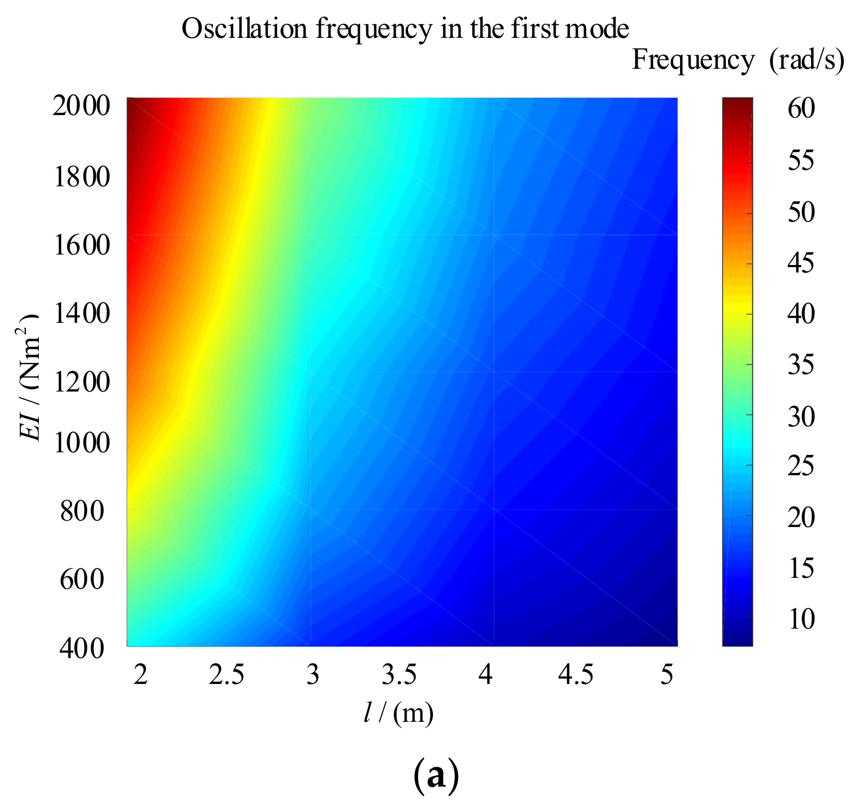
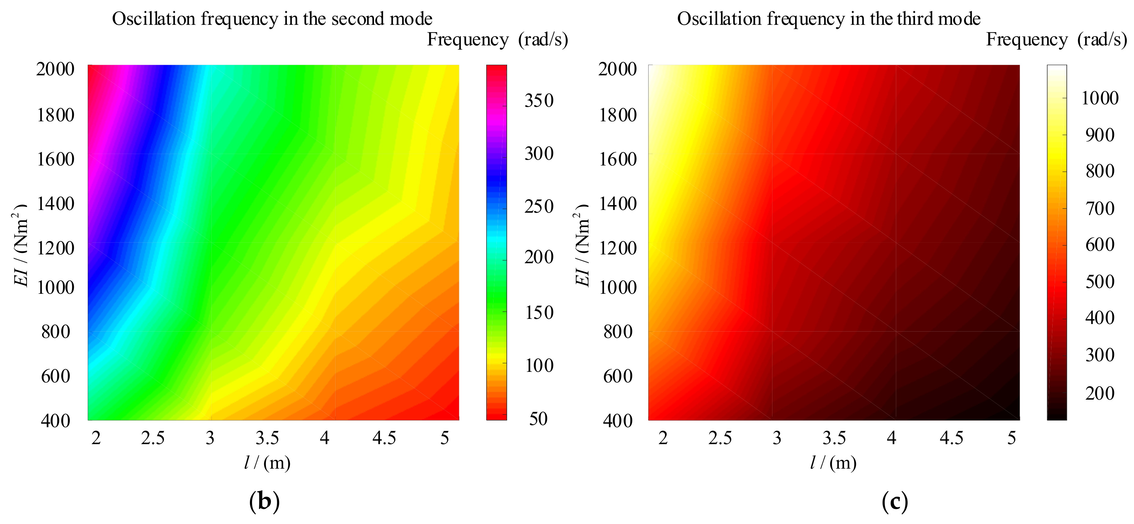
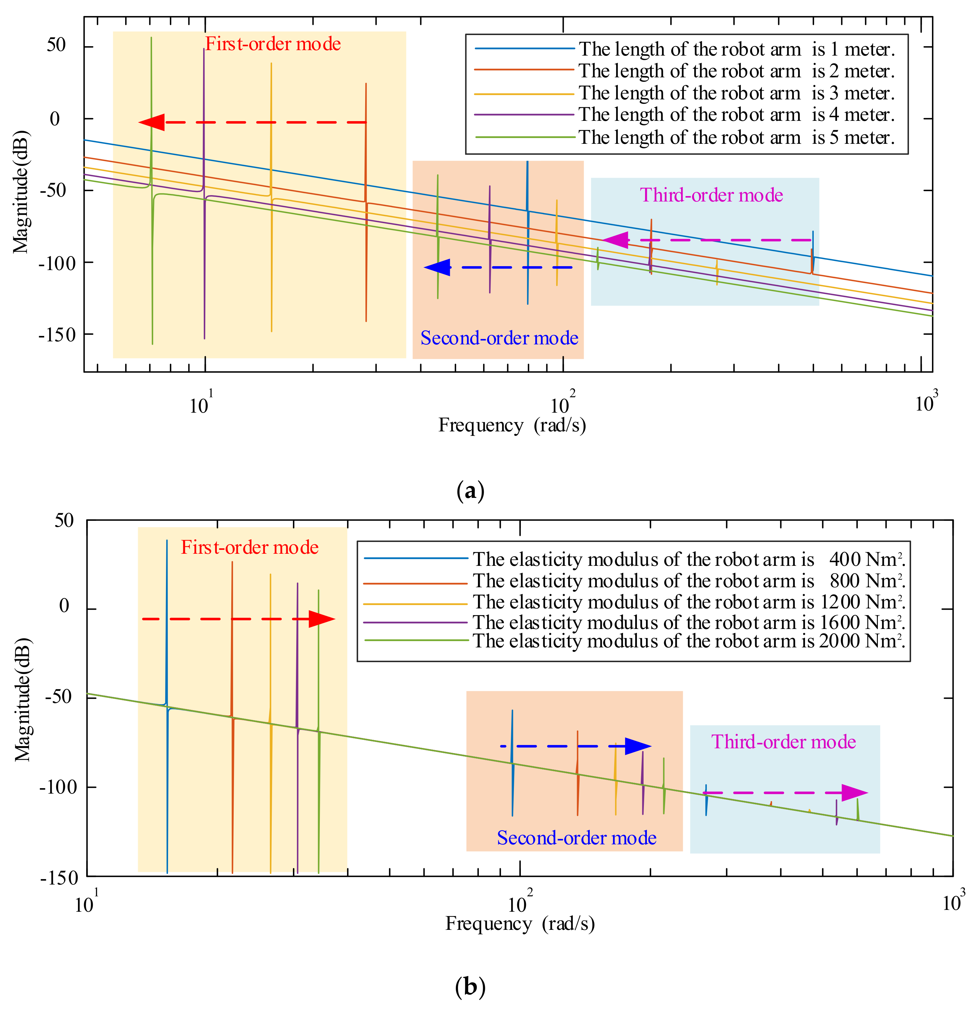
The length and elastic modulus reflect the flexibility of manipulators. They also have an impact on the resonance frequency of the servo system. According to Equation (37), the influence of the flexible manipulator’s physical parameters on the resonant frequency can be obtained, as shown in Figure 9. According to Figure 9, the flexible manipulator’s resonance frequency decreases as the length increases and increases as the elastic modulus increases. The conclusion drawn in Figure 9 is the same as that in Figure 4. It can be seen that the stronger the flexibility of manipulators, the smaller the resonance frequency. Vibration is more likely to occur in the low-frequency phase.

5.2. The Influence of Coefficients of the Pole on the Rotation Angle

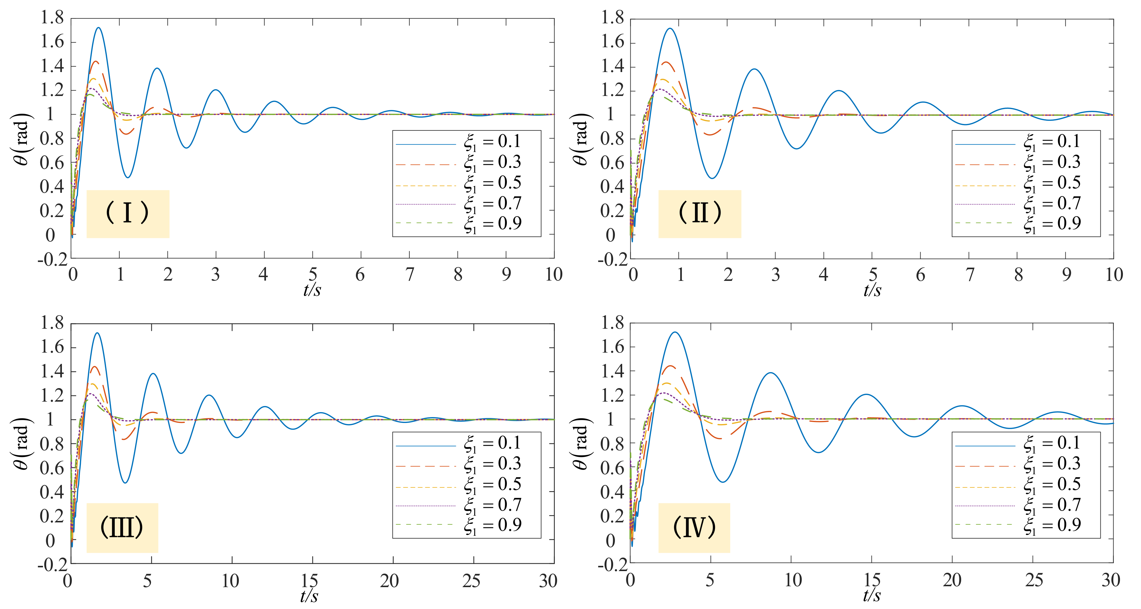
Before using the RBF neural network to compensate for the uncertain items, the PD controller parameters need to be determined. The value of the controller parameter directly affects the control accuracy of the servo system output. In this paper, the pole placement strategy is used to optimize the parameters of the PD controller. It provides a theoretical basis for the parameter selection of the PD controller. According to the pole placement strategy, the selection of controller parameters can be attributed to selecting the damping coefficient of poles. Different damping coefficients of poles will affect the output of the servo system. The unit step signal is used as the system’s input signal to obtain the variation rules of rotation angle with time, as shown in Figure 10. Among them, the numerical simulation selected 4 different parameters, as shown in

Table 1. Parameters of flexible manipulators.

Parameters	Condition1	Condition 2	Condition 3	Condition 4
Flexible load length l/m	2	3	4	5
Flexible load mass m/kg	1	1	1	1
Elastic modulus of flexible load EI/Nm2	2000	1600	800	400
Linear density of flexible load ρA/kg/m2	0.5	0.3333	0.25	0.2
Flexible load inertia Ia/kgm2	1.333	3	5.333	8.33
Flexible modal coupling coefficient Fa1/kg1/2m	1.1376	1.7064	2.27521	2.8440
Modal frequency of the flexible load ω1/rad/s	55.5869	27.0633	12.4296	6.2889
Characteristic root of modal function β1	0.9375	0.625	0.4688	0.375

.

According to Figure 10, it can be seen that the variation rule of the rotation angle is not only related to the damping coefficient of poles but also closely related to the length and elastic modulus of flexible manipulators.

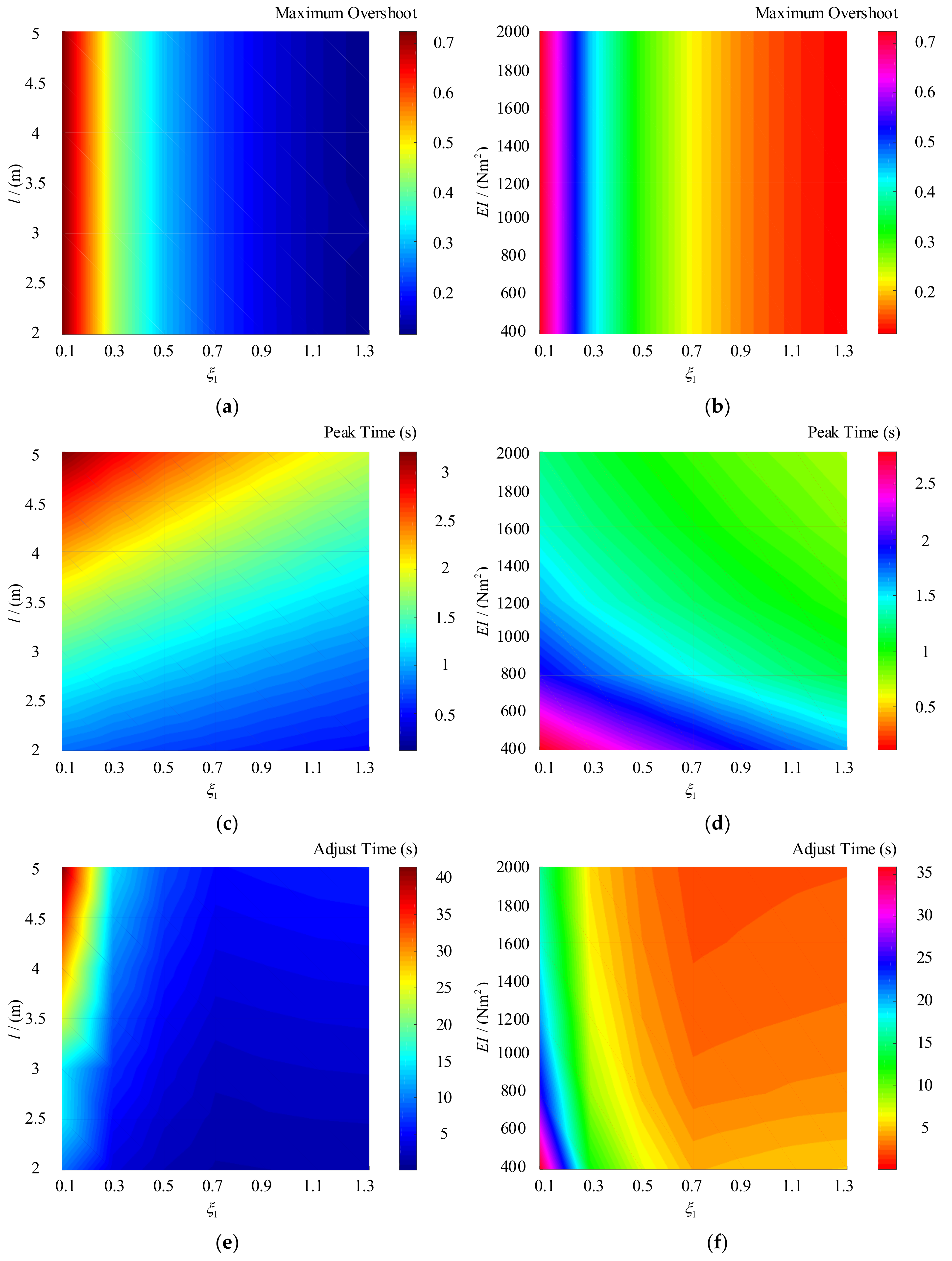
In this paper, three indexes of maximum overshoot, peak time, and adjustment time are selected to evaluate the output characteristics [21]. Among them, the maximum overshoot reflects the system’s dynamic accuracy; the peak time and adjustment time reflect the rapidity of the system. If the maximum overshoot is smaller, the system is more stable. On the contrary, it shows that system stability is poor. If the peak time and adjustment time are shorter, the system rapidity is better. On the contrary, it indicates that the system reflects slowly. The influence law of the length, elastic modulus, and damping coefficient of poles on the evaluation index is shown in Figure 11.

According to Figure 11, as the flexible manipulator’s length increases, the maximum overshoot of rotation angle does not change, but the adjustment time and peak time increase significantly. It can be seen that with the rise in the length of flexible manipulators, the flexibility of the manipulator rises, and it takes a long time to stabilize the system. With the increase of flexible manipulators’ elastic modulators, the maximum rotation angle does not change, but the adjustment time and peak time decrease. It can be seen that with the increase of the elastic modulus, the flexibility of manipulators is weakened, and it takes a shorter time to stabilize the system. However, the damping coefficient of poles has a greater influence on the overshoot. With the increase of the damping coefficient of poles, the overshoot decreases gradually. The damping coefficient of poles has a weak effect on the adjustment time and peak time. According to Figure 11, it is appropriate to select poles’ damping coefficient between 0.5 and 0.7. In this interval, the system can obtain a faster response and receive a smaller overshoot.

5.3. Control Method Based on the Combination of RBF Neural Network and Pole Placement Strategy

In order to verify the effect of the combination control method, the parameters in Table 1 are selected to carry out a numerical simulation experiment. The simulation experiment takes the sine function as the input signal and obtains a change in the rotation angle over time, as shown in Figure 12. The influence of the manipulator’s length and elastic modulus on the rotation angle error under different control strategies is shown in Figure 13.

According to Figure 12, if the pole placement strategy is used alone, stable tracking can be achieved when manipulators’ length is small. With the increase of the length of manipulators, pole placement’s control strategy cannot satisfy the precise tracking. However, after using the neural network to compensate for the uncertain items, the combination control method can ensure the system’s stability.

According to Figure 13, it can be seen that the control method using pole placement strategy alone will have a large error. Additionally, the error increases as the length of manipulators increases. The error decreases with the increase of elastic modulus. It is shown that the control method using pole placement strategy can only satisfy the condition of low flexibility. The control effect is not suitable for the situation of large flexibility. However, the combined control method is not affected by the flexibility of manipulators. The combined control method can obtain a better control effect in any cases.

5.4. Experiment

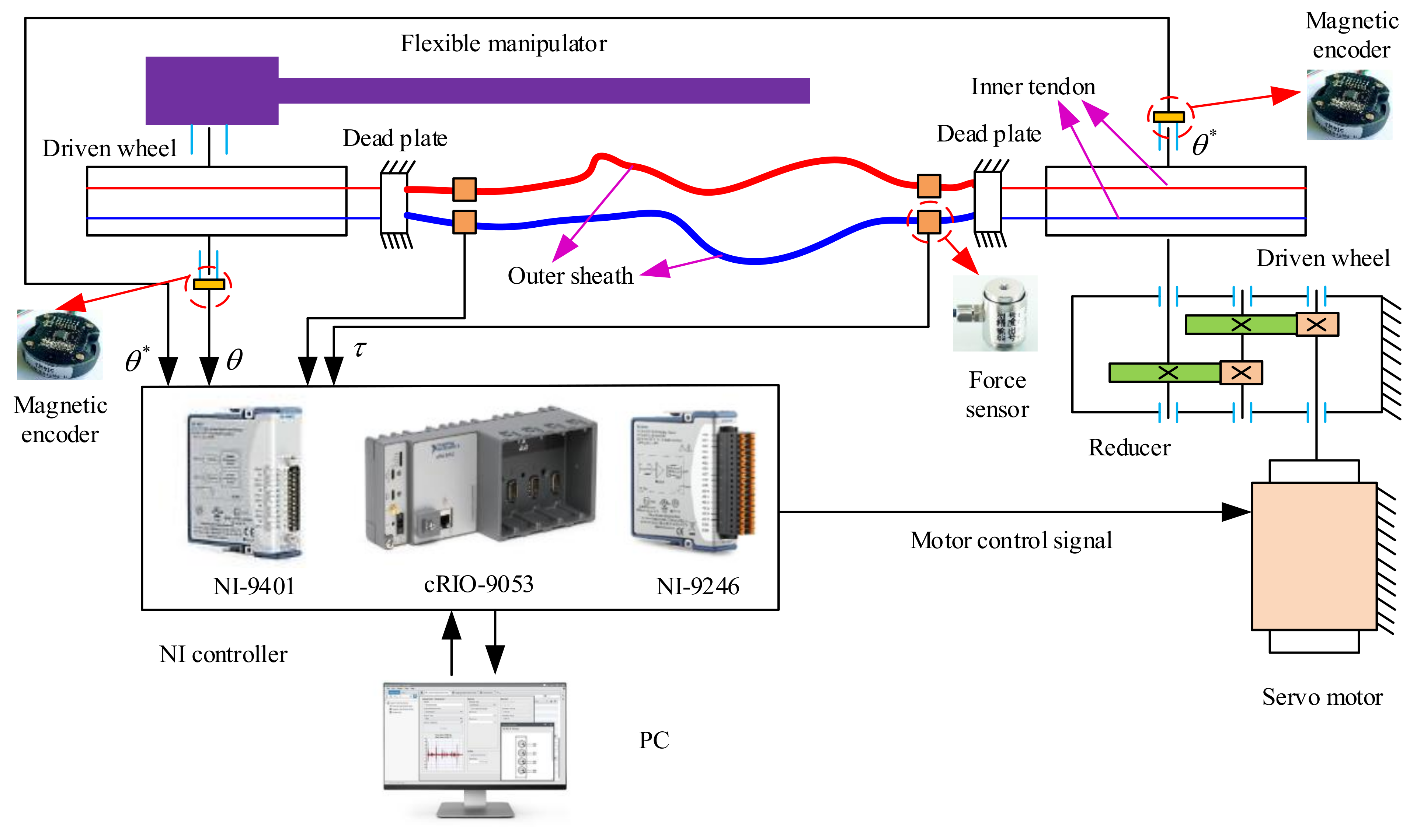
This paper builds an experimental platform to verify flexible manipulators’ control strategy, as shown in Figure 14. The experimental platform is composed of a servo motor, a transmission tendon-sheath, and a flexible manipulator. The tendon-sheath transmits the input torque generated by the servo motor to the flexible manipulator. The input torque of the flexible manipulator can be accurately calculated through the tension sensor on the tendon-sheath. The control platform uses CRIO-9053 as the lower computer that inputs the collected feedback signals into LabVIEW’s control program. Simultaneously, the control program’s output signal is transmitted to the NI-9246 module to control the output torque. Magnetic encoders collect the feedback signal. The magnetic encoder is installed at the back of the flexible manipulator to collect the angle signal. The control principle of the experimental platform is shown in Figure 15.

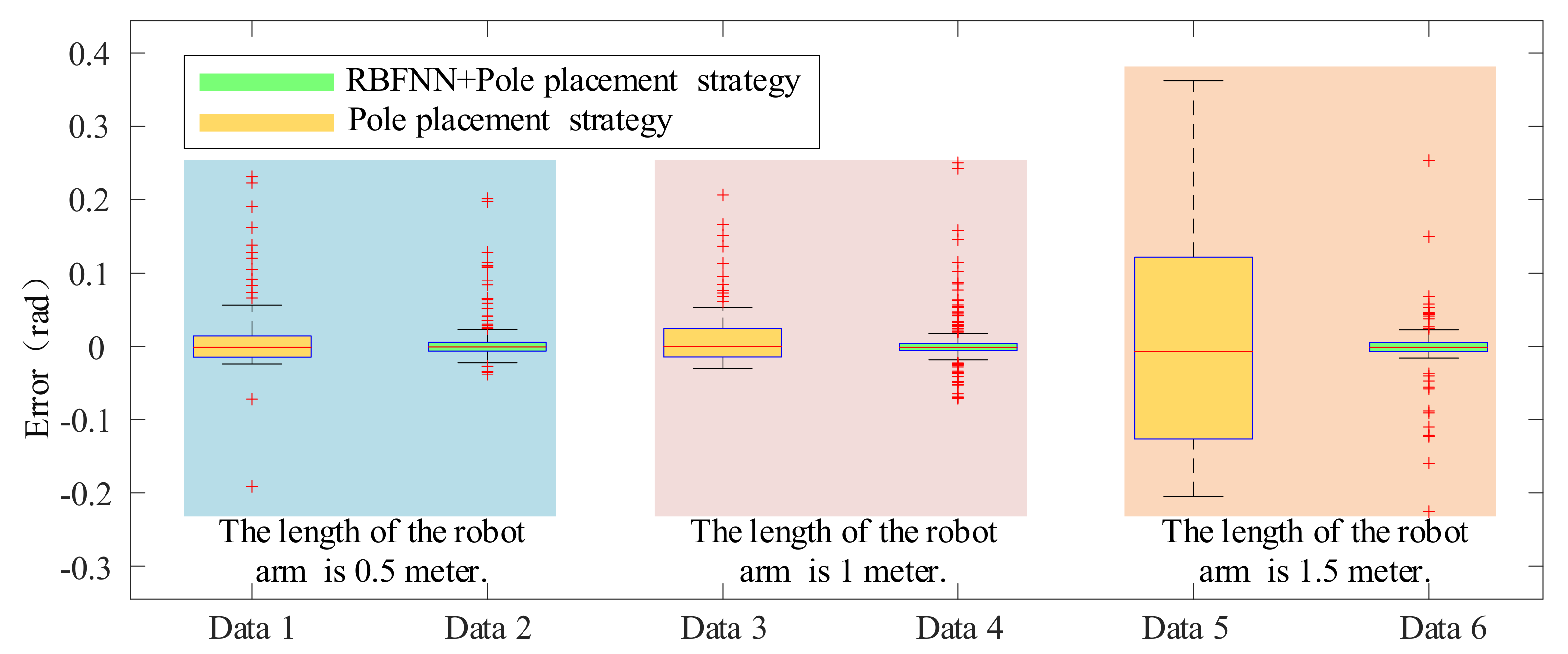
The flexible beam is used to simulate the flexible manipulator in the control experiment platform. Flexible beams with lengths of 0.5, 1, and 1.5 m are used to simulate flexible manipulators of different lengths. Two different control methods are used to experiment with rotation angle control. One of the control methods is to use the pole placement strategy alone, and the other is to use the combined control method. The relationship between the rotation angle with a length of 0.5 m and its error are shown in Figure 16. Six groups of experimental data can be obtained through the experiment. The statistical results of the rotation angle errors of the experimental data groups are shown in Figure 17. What is more, the error indicators of six groups of experimental data can be obtained as shown in

Table 2. Error indicators of six groups of experimental data.

	Robot Arm Is 0.5 m		Robot Arm Is 1 m		Robot arm Is 1.5 m
Error Indicators	Combined Control Strategy	Pole Placement Strategy	Combined Control Strategy	Pole Placement Strategy	Combined Control Strategy	Pole Placement Strategy
Error standard deviation	0.0337	0.0967	0.0407	0.0634	0.1741	0.2654
Mean error	0.0023	0.0041	0.0018	0.0053	0.0034	0.2654

.

It can be seen from Figure 16 that the combined control method has a smaller error. According to Figure 17 and Table 2, it can be seen that the combined control method can make the flexible beams of different lengths get smaller tracking errors. However, the pole placement strategy alone cannot guarantee the flexible beam’s tracking accuracy in the case of a long length. Therefore, the effectiveness of the control strategy proposed in this paper is verified through experiment.

6. Conclusions

In this paper, a dynamic model of flexible manipulators with gravity is established. The innovation of this paper is to consider the factor of gravity and the combined control strategy is used to improve the motion accuracy. The control method combining the pole placement strategy and the RBF neural network is applied to reduce the fluctuation of the rotation angle of flexible manipulators. Then, the motion precision of flexible manipulators is improved. Among them, the RBF neural network is used to distinguish the uncertain items of the system. The uncertain items include both the flexible factors and the time-varying characteristics of the dynamic parameters. Simulation analysis and experiments show that the proposed control method can effectively suppress the rotation angle’s vibration and improve the motion accuracy of the end-effector. The specific conclusions are as follows:

(1)

Gravity factors will seriously affect the input torque of flexible manipulators. If flexible manipulators move in the vertical plane, the gravity factor should be taken into account.

(2)

Its length and elastic modulus determine the flexibility of manipulators. The PD controller can control the manipulator with less flexible. The pole placement strategy is used to optimize the PD controller’s parameters to obtain a stable output of the rotation angle. However, for the manipulator with strong flexibility, the pole placement strategy cannot receive a stable output of the rotation Angle. Using the RBF neural network control strategy to identify the uncertain items containing the flexible factors can effectively reduce flexibility.

(3)

The simulation and experimental results show that the control method combined with the RBF neural network and the pole placement strategy can effectively reduce the error of the flexible manipulator’s rotation angle. According to the Table 2, compared with pole placement strategy alone, the mean error is reduced by nearly 60%. Therefore, the combined control method can effectively reduce the angle error. Therefore, the control method proposed in this paper can effectively improve the control accuracy of the flexible manipulator.

This paper uses the control method to improve the motion accuracy of flexible manipulators. It is hoped that the vibration isolation device can be added between flexible manipulators and end-effectors in the future. In this way, the motion accuracy of flexible manipulators can be improved.