Article

Subsurface Temperature Estimation from Sea Surface Data Using Neural Network Models in the Western Pacific Ocean

1
College of Information Science and Technology, Qingdao University of Science and Technology, Qingdao 266061, China
2
Research Institute for Mathematics and Interdisciplinary Sciences, Qingdao University of Science and Technology, Qingdao 266061, China
3
School of Mathematics and Physics, Qingdao University of Science and Technology, Qingdao 266061, China
4
Marine Science Data Center, Institute of Oceanology, Chinese Academy of Sciences, Qingdao 266071, China
5
Center for Ocean Mega-Science, Chinese Academy of Sciences, Qingdao 266071, China
*
Authors to whom correspondence should be addressed.
Mathematics 2021, 9(8), 852; https://doi.org/10.3390/math9080852
Submission received: 2 March 2021 / Revised: 7 April 2021 / Accepted: 10 April 2021 / Published: 14 April 2021
(This article belongs to the Special Issue Artificial Intelligence and Big Data Computing)

Abstract

:
Estimating the ocean subsurface thermal structure (OSTS) based on multisource sea surface data in the western Pacific Ocean is of great significance for studying ocean dynamics and El Niño phenomenon, but it is challenging to accurately estimate the OSTS from sea surface parameters in the area. This paper proposed an improved neural network model to estimate the OSTS from 0–2000 m from multisource sea surface data including sea surface temperature (SST), sea surface salinity (SSS), sea surface height (SSH), and sea surface wind (SSW). In the model experiment, the rasterized monthly average data from 2005–2015 and 2016 were selected as the training and testing set, respectively. The results showed that the sea surface parameters selected in the paper had a positive effect on the estimation process, and the average RMSE value of the ocean subsurface temperature (OST) estimated by the proposed model was 0.55 °C. Moreover, there were pronounced seasonal variation signals in the upper layers (the upper 200 m), however, this signal gradually diminished with increasing depth. Compared with known estimation models such as the random forest (RF), the multiple linear regression (MLR), and the extreme gradient boosting (XGBoost), the proposed model outperformed these models under the data conditions of the paper. This research can provide an advanced artificial intelligence technique for estimating subsurface thermohaline structure in major sea areas.

1. Introduction

About 93% of the energy of global warming is stored in the oceans, where heat changes and redistribution in the subsurface and deep ocean (300–2000 m) play an important role in the global warming process [1,2,3,4]. In addition, dynamic processes within the ocean are very complex, and many important physical oceanic phenomena and dynamic processes exist in a certain depth range below the surface [5]. Therefore, the thermal structure of the ocean subsurface is crucial for the study of the mechanisms and dynamic processes of internal ocean phenomena.
Current satellite remote sensing is one of the effective ways to detect the ocean environment on a large scale and long time series, and it has been widely used in the field of marine scientific research [6]. However, the observations can only obtain the information of ocean surface and are unable to directly detect information inside the ocean. Compared with remote sensing observations, ocean-based in situ observation data, while precise, are distributed unevenly and discontinuously in time and space, and cannot meet the requirements for the study of internal ocean dynamic processes [7,8]. Therefore, combining remote sensing data with multi-disciplinary ocean observational data to estimate the ocean subsurface thermal structure (OSTS) is a meaningful and important topic [6].

2. Related Work

Many scholars have continuously been trying to estimate the OSTS based on different observation data and numerical models from sea surface parameters [9,10,11,12]. In the early stage of this study, the OSTS was mainly evaluated with individual sea surface parameter. For example, Wunsch et al. and Kao obtained the ocean subsurface thermal structure based on a dynamical model with in situ observations [9,10]. Khedouri and Fiedler et al. investigated the purely statistical relationship between the sea surface temperature (SST) and ocean subsurface temperature (OST) profiles [11,12]. Chu et al. constructed a parametric model based on the stratified structure analysis of observed temperature profiles, using the model to obtain the SST from satellite data to estimate the relationship between subsurface parameters such as the OST, mixed layer depth (MLD), and temperature gradient in the thermocline [13,14,15,16]. With development of the research, a variety of sea surface parameters were used to reconstruct the OSTS. For example, Willis et al. estimated stereo height, thermal storage, and subsurface temperature variability from measured data combined with large-scale profile data [17]. Jeong et al. used multivariate satellite remote sensing data to reconstruct the 3D ocean thermal structure through the use of multiple linear regression (MLR) models and analyzed the change of the MLD during the global warming interval [18]. However, the previous studies based on numerical models are complicated and time-consuming. If appropriate algorithms are used, a combination of multi-disciplinary ocean observational data can be applied to directly and accurately estimate the subsurface dynamic fields [5].
In recent years, with the development of remote sensing data, model simulation data, and Argo datasets, multisource sea surface data with a high level of quality have become more and more abundant. Artificial intelligence applications in the oceanography field have been widely studied [19,20]. In particular, machine learning methods based on various sea surface parameters have been used to reconstruct the OST with many outstanding results [6,21,22,23,24]. Ali et al. used neural networks to estimate the internal thermal structure of the ocean by using the SST, sea surface height (SSH), wind stress, net radiation flux, and heat flux data from the Arabian Sea mooring system [21]. Su et al. used classical machine learning methods such as the random forest (RF), the support vector regression (SVR), and other artificial intelligence methods to estimate global ocean subsurface temperature anomalies (STAs) based on multisource satellite observations [22,23,24]. Recently, Su et al. also estimated the global ocean subsurface temperature and salt anomalies using the extreme gradient boosting (XGBoost) model by combining sea surface remote sensing data and Argo buoy observations [6]. There have been other valuable studies on the ocean’s interior that have employed multisource observations [19,20,25].
Most of the existing studies are oriented to the global ocean and cannot accurately describe the variation pattern of a local ocean area. In particular, there are few researches on the estimation models for major ocean areas with complex dynamic processes [22,23,24]. Moreover, most of the previous models are traditional machine learning models based on a few sea surface parameters to estimate the subsurface information. Thus, the estimation models themselves and their accuracy and reliability still show much room for improvement [24]. Based on the above observations, in this paper, we selected the western Pacific Ocean, where complex oceanic variability exists, as the research object, and proposed a novel artificial neural network (ANN) model to estimate the subsurface three-dimensional temperature structure of this area using the SST, SSH, sea surface wind (SSW), and sea surface salinity (SSS) as input variables. We extended the reconstruction space of the model to 2000 m below the sea surface (the maximum depth of Argo observation data). To improve the estimated OST, a series of experiments were conducted for the parameter selection and network architecture in this paper. The model was further compared with the MLR, RF, and XGBoost to evaluate the accuracy and reliability of the proposed model. Finally, we quantitatively analyzed the effects of sea surface parameters on the estimation models.

3. Motivation

The strongest El Niño in the past 60 years occurred in the central and eastern Pacific Ocean with a Nino 3.4 index of 3.1, having a significant impact on the global climate [26,27]. As the research progresses, the study of El Niño has been gradually extended to the western Pacific region. The tropical western Pacific Ocean is the region with the highest global sea surface temperature and is the largest global heat source. Many scholars found that the SST in the western Pacific Ocean is closely related to the El Niño phenomenon occurring in the central and eastern Pacific Ocean [28,29,30,31], and the important role of the SST variability in the tropical western Pacific Ocean was emphasized in the El Niño-Southern Oscillation (ENSO) cycle mechanism [32,33]. In addition, the peak of ENSO-related SST anomalies in the western Pacific usually lags behind the peak in the central tropical Pacific by one to two seasons, a phenomenon that is closely linked with the frequent occurrence of droughts and floods in East Asia in recent decades [34,35]. Cao et al. found that the abrupt variability of the East Asian summer winds were clearly influenced by the ENSO phenomenon in this ocean, on an interannual scale [36]. Therefore, the SST variability in the western Pacific Ocean is important for studying the ENSO cycle mechanism, East Asian drought and flood disasters, and East Asian summer wind variability.

4. Methods

4.1. Data

In this study, the SST, SSS, SSH, SSW u, and SSW v components (UW and VW, respectively) are used to estimate the OST in this paper. Among them, the SST and SSS are from the Argo monthly gridded data provided by the International Pacific Research Center (IPRC) from January 2005 to December 2016 (http://apdrc.soest.hawaii.edu/projects/Argo/data/gridded/On_standard_levels/index-1.html accessed on 2 March 2021). The Argo data had a spatial resolution of 1° and contained 27 vertical standard levels of the ocean interior (from the surface to a depth of 2000 m). The SSH gridded dataset at 0.25° resolution was published by Aviso with the support of the National Space University Center (http://www.aviso.altimetry.fr/en/data/products/sea-surface-height-products/global/ accessed on 2 March 2021). The UW and VW components are derived from the Ocean Reanalysis System 4 (ORAS4) product provided by the European Centre for Medium-Range Weather Forecasts (ECMWF) from January 2005 to December 2016, which is built on the Nucleus for the European Modeling of the Ocean (NEMO) model using the Variable Fraction Data Assimilation System, designed to provide reliable data for data analysis of the global ocean [37,38,39,40,41] (http://apdrc.soest.hawaii.edu/erddap/griddap/hawaii_soest_3512_a2e8_e3ce.html, http://apdrc.soest.hawaii.edu/erddap/griddap/hawaii_soest_e18a_18c8_bdcb.html accessed on 2 March 2021).
We use interpolation to unify these data with a resolution of 0.1°. If any variable was null at the same position this node was deleted. The number of valid data nodes for each month after processing was about 300,000 and there were 144 months of data from 2005 to 2016. The data from 2005 to 2015 were used as the training set and the 2016 data as the testing set. In order to equally weight all variables, all data were normalized before being inputted to each model. Table 1 summarizes all input variable data sources used in this study.

4.2. Artificial Neural Network

In order to estimate the OST, we established an ANN model consisting of an input layer, an output layer, a first hidden layer with 30 neurons, and a second hidden layer with 20 neurons. The activation function of the neurons in the hidden layer is the Relu function. Compared with the Sigmoid function as the activation function [42], the Relu function is more consistent with the biological neural activation mechanism without complex exponential operations. The Relu function has the advantages of low computational cost and fast convergence, and can avoid gradient explosion and disappearance problems.
In determining the number of neurons and hidden layers, we used a grid search strategy to determine the optimal structure of the ANN. We tested various structures of neural networks with increasing numbers of neurons from 5 to 30 (each increase of 5) and hidden layers from 1 to 4 layers. A severe overfitting problem was found when the number of hidden layers reached three, while the loos value decreases significantly without overfitting if the number of hidden layers increased from one to two. Based on these analyses, we chose a neural network structure with 30 neurons in the first hidden layer and 20 neurons in the second hidden layer. In addition, to avoid the overfitting of the ANN during the training process, we used the L2 regularization algorithm to perform the training process. Compared with traditional neural network methods, L2 regularization is more suitable for fitting complex nonlinear regression functions and does not require a cross-validation process to ensure generalizability [43], which is why we did not determine the validation set during the training process.

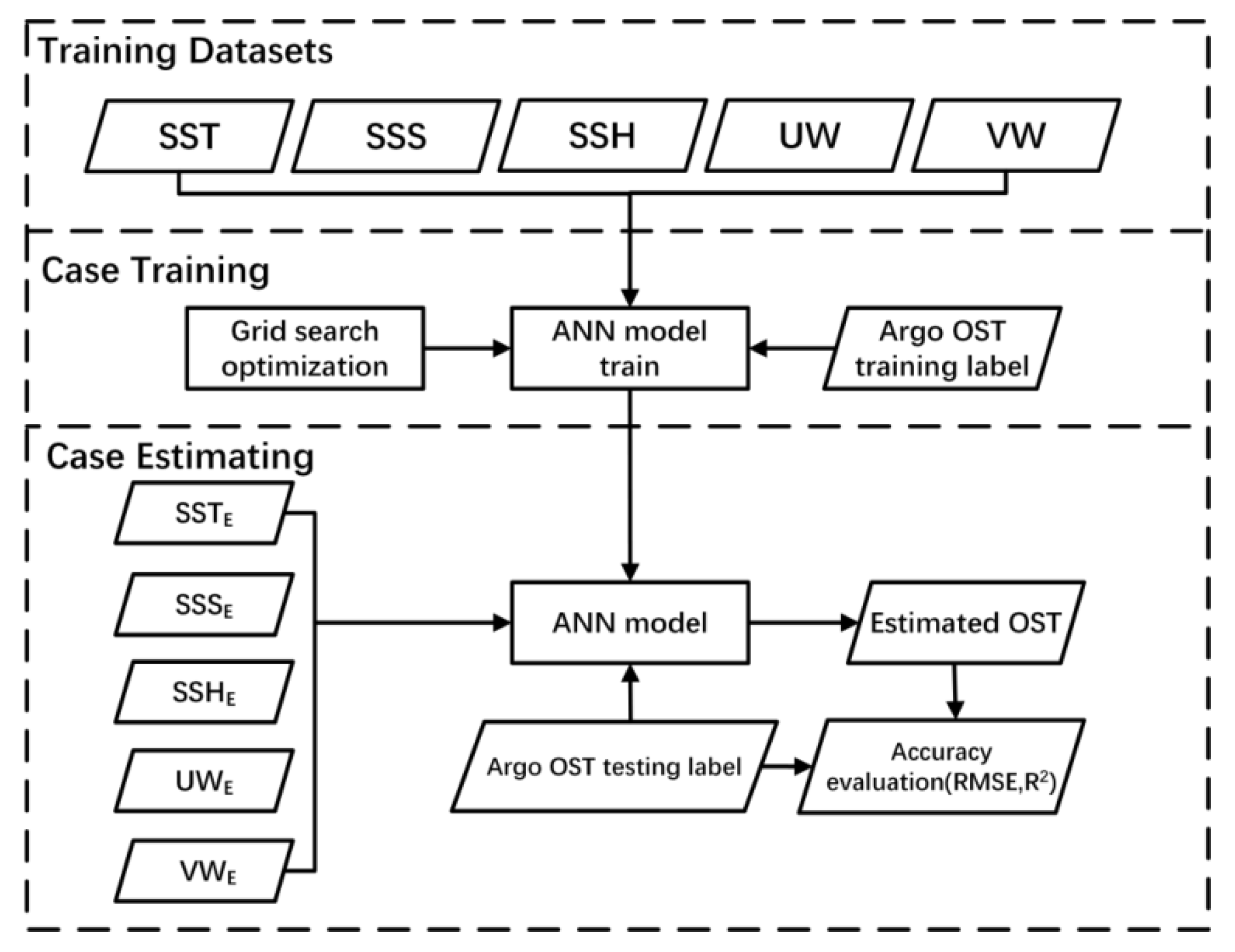
4.3. Experimental Step

In this paper, we fused sea surface parameters from multisource observations (i.e., the SSS, SSH, SST, UW, and VW) to estimate the subsurface thermal structure in the western Pacific Ocean via the ANN model. The flow chart of the estimated OST at different depth levels is shown in Figure 1. The experiment was divided into three stages. The first stage was the establishment of training and testing sets. The five sea surface parameters were used as independent input variables of the ANN model, and the ocean subsurface temperature observed by Argo was used as the training and testing labels. These sets were divided by month, and the data from 2005 to 2015 were used as the training set and the 2016 data were used as the testing set. The second stage involved the training of the ANN model. The grid search strategy was used to tune the hyper-parameters of the model and the estimation model with optimal parameters was established. The third stage was the estimation of the OST based on the model. To analyze the effects of different combinations of sea surface parameters on the OST, the five experiments (Cases 1–5) including different input variables were designed, as shown in Table 2. To compare the performance of the ANN model with some popular machine learning models, the XGBoost model [6], the MLR model [18], and the RF model [24] were respectively used in Case XG, Case LR, and Case RF, as also shown in Table 2. The accuracy and reliability of the model were evaluated by the RMSE and determination coefficient (R2).

5. Results and Discussion

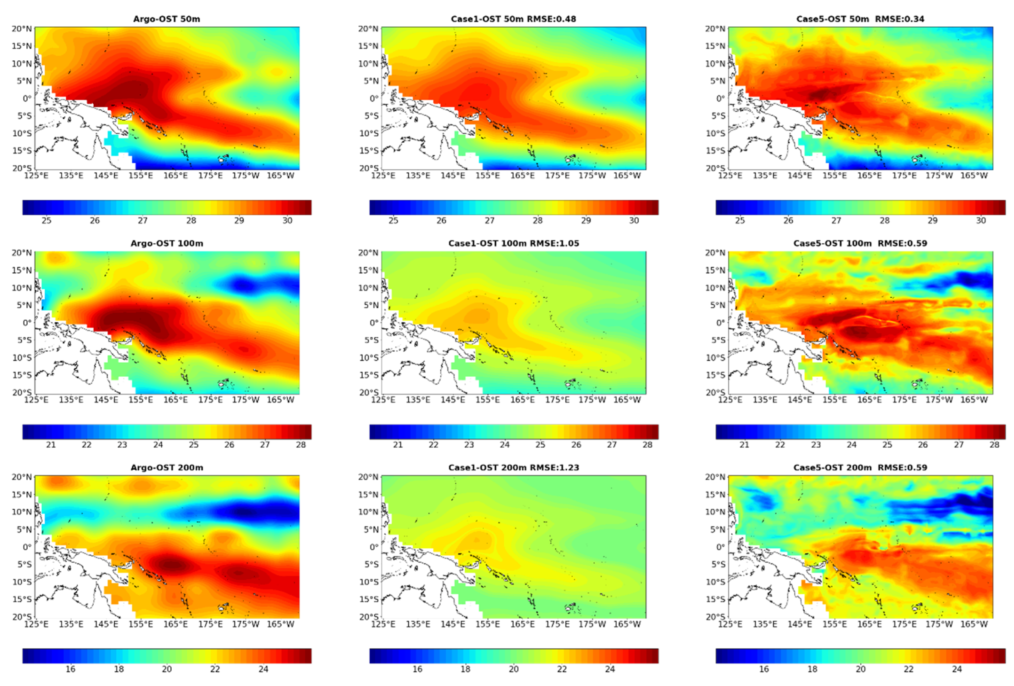
5.1. Results of the Estimated OST for Different Cases

As an example of the application of the ANN model, Figure 2 shows the spatial distribution of the Argo-derived and ANN-estimated OST for Case 1 and Case 5 in November 2016 at several depth levels (50 m, 100 m, and 200 m). The RMSE values of Case 1 to Case 5 at 50 m, 100 m, and 200 m depths are shown in Table 3. From Figure 2 and Table 3, it can be seen that the error of Case 1 increases sharply with the depth. This indicates that although the ANN model can effectively capture the temperature in the shallow sea area [42], there is a huge error in the estimation effect of the model relying only on the SST in the sea area where complex physical ocean motion exists. For example, in Case 1, the signals of the low-temperature sea area and warm pool at 100 m and 200 m depths are much weaker than those observed by Argo, or even disappear. As shown in Table 3, the RMSE values of Case 5 at 50 m, 100 m, and 200 m were about 0.34, 0.59, and 0.59 °C, respectively. The comparison between the Argo-observed OST and Case 5 also showed that there were only some minor differences between them. In addition, with the increase of depth, the change of RMSE tended to be gentle. From 500 m to 2000 m, the average RMSE of Case 1 to Case 5 was 0.97, 0.96, 0.75, 0.94, and 0.68 °C. On the whole, the accuracy of the ANN model still needs to be improved in the warm pool and the highest temperature area of the western Pacific Ocean near the equator.
In Table 4, the average RMSE of the estimated OST at 26 depths for different cases are summarized. Among all the cases, Case 5 presented the smallest RMSE (across all depths, 0.55 °C) and could improve the RMSE up to 31% in comparison to Case 1. Namely, the estimation accuracy of the model keeps improving and there is no redundancy in the input variables. It can be seen that the ANN estimation model in Case 5 can more accurately fit the nonlinear relationship between the input and output variables in the western Pacific Ocean.

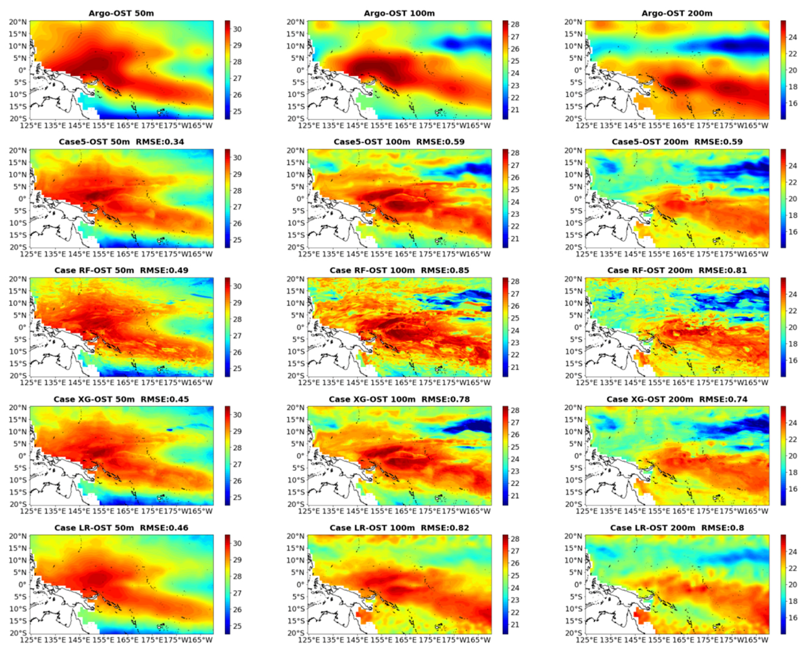
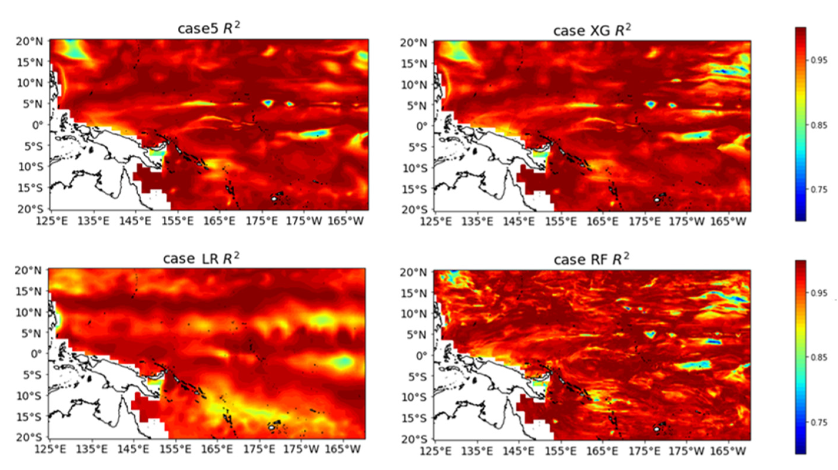
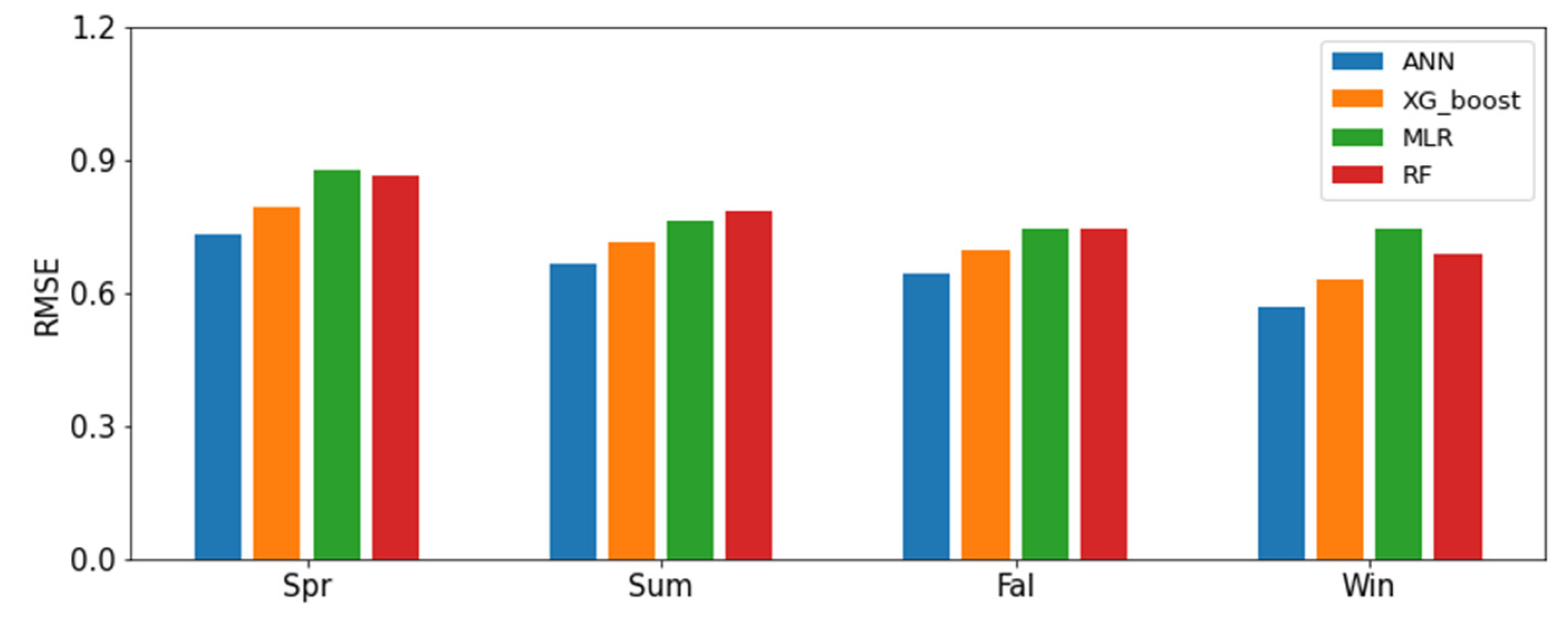
5.2. Accuracy Comparison of Different Models

The proposed ANN model (Case 5) was compared with several popular machine learning models including the XGBoost [6] (Case XG), the MLR [18] (Case LR), and the RF [24] (Case RF). The parameter values of each estimation model are shown in Table 5.
Figure 3 presents a comparison between the Argo-observed and estimated OST of different models at 50 m, 100 m, and 200 m in November 2016, respectively. Compared with the ANN model, the other three models have larger RMSE regardless of the depth, which is due to the fact that these models are good at capturing smooth, linear dynamic processes in the ocean’s interior. However, there are many nonlinear dynamic processes in the western Pacific Ocean due to the smaller Koch parameter and the faster response of the tropical ocean to atmospheric anomalies in this region [44], which leads to the low estimation accuracy of these models.
Table 4 also shows the average RMSE of the estimated OST at 26 depths for Case 5, Case RF, Case XG, and Case LR. Compared with the other cases, the average RMSE of Case 5 was reduced by 0.13, 0.16, and 0.20 °C, respectively. From Figure 3, it can also be found that the ANN model outperforms the other models with increasing depth. In particular, there was a large difference between the RF and XG-Boost models in the low-temperature sea areas of 175° W~165° W and 7° N~15° N, while the MLR model was almost unable to estimate the OST in the low-temperature sea area. In addition, all four estimation models have the problem that they cannot accurately estimate the core region of the warm pool, i.e., the maximum temperature of the warm pool estimated by the models is lower than that observed by Argo. This suggests that there may be nonlinear physical ocean motion in the warm pool that cannot be captured by the estimation model. However, by comparison, the proposed ANN model has better estimation accuracy and reliability.
In addition, we also compare the R2 distributions for all different models, as shown in Figure 4. The RF and XG-Boost models have low R2 values near the low-temperature sea areas, implying that these models also cannot accurately estimate the OST in these areas. The R2 values of the MLR model is also lower in the sea area from 10° S to 20° S, implying that the MLR model cannot capture the nonlinear physical ocean motion in this region. Overall, the ANN model has better performance than the other models in the ocean region.

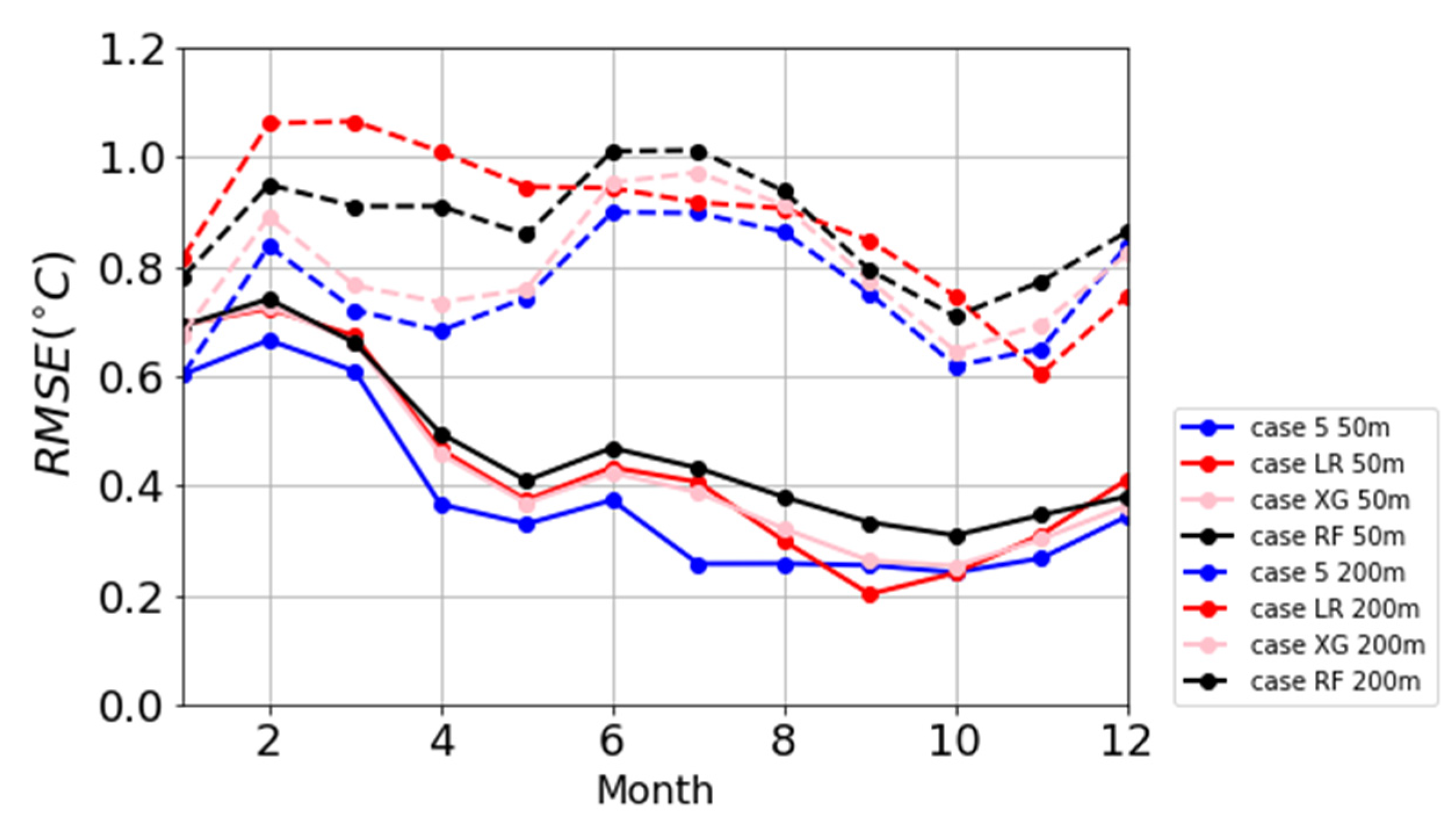
5.3. Comparison of Time Series Results

In Section 5.1 and Section 5.2, data for one specific month was used to evaluate the performance of the model. Next, in order to compare the estimation effectiveness of the four estimation models with temporal and spatial variations, we implemented these models at different depth levels in the four seasons and 12 months of 2016, respectively. The average RMSE of the OST at 26 different depths (0–2000 m) within the western Pacific Ocean in the four seasons are shown in Figure 5. As shown in Figure 5, the average RMSE of the OST estimated by the ANN model was about 0.73, 0.66, 0.64, and 0.56 °C for spring, summer, autumn, and winter, respectively, implying that these values were lower than those of the other three models regardless of the season. The results showed that at seasonal time scales, the proposed ANN model can better estimate the OST in the western Pacific Ocean, where the physical ocean phenomena are complex.
The RMSE of the OST estimated by the ANN, MLR, XG-Boost, and RF at 50 m and 200 m depths for all months of 2016 in the western Pacific Ocean are given in Figure 6. Compared with the XG-Boost, MLR, and RF models, the average RMSE values at 50 m were reduced by 0.05, 0.06, and 0.09 °C, respectively. The advantage of the ANN model was gradually obvious with increasing depth, and the average RMSE values at 200 m were reduced by 0.04, 0.13, and 0.12 °C, respectively. The results showed that the accuracy of the ANN model was relatively high for all months of 2016, suggesting that the proposed ANN model has a good seasonal applicability to the OST estimations.

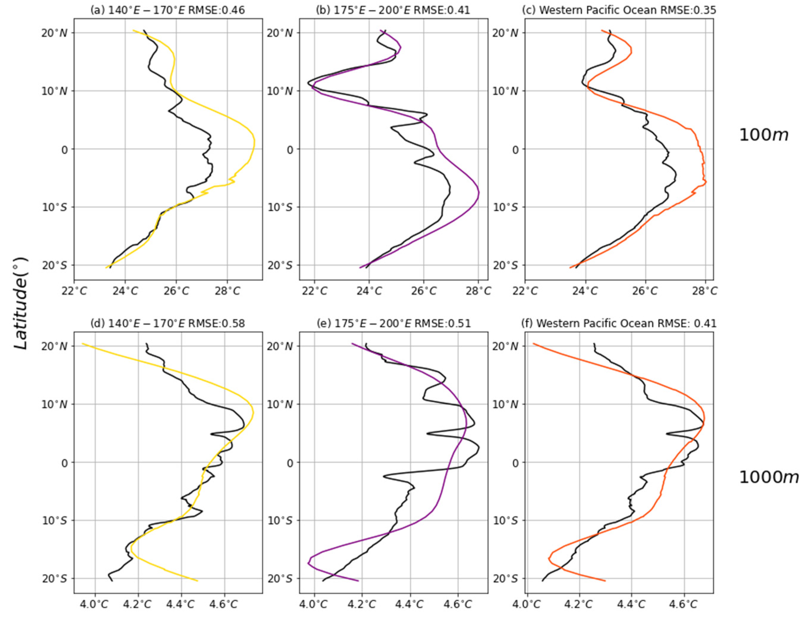
5.4. Evaluation on Effect of Specific Sea Areas

To explore the estimation performance of the ANN model for some specific sea areas in the western Pacific Ocean, such as the warm pool and the low-temperature sea area, Figure 7 shows the distribution of the Argo-observed and estimated OST profiles at 100 m and 1000 m for these areas and the whole sea region in November 2016. At 100 m and 1000 m, the RMSE values were 0.46 °C and 0.58 °C for the warm pool and 0.41 °C and 0.51 °C for the low-temperature sea area, respectively, implying that the ANN estimation model has better results in the low-temperature sea areas in comparison with the warm pool. In the warm pool, the relatively accurate trend of the OST cannot be obtained by using the ANN model at 100 m, and the estimated OST values are significantly smaller than the Argo-observed OST. In addition, it can be seen from the results that the estimation accuracy of the model decreases with the depth, which should be related to the reduced correlation between the temperature in the ocean depths and the sea surface parameters.

5.5. Correlation Analysis between the OST and Sea Surface Parameters

The previous analysis shows that the estimation effectiveness of the ANN model is closely related to the input sea surface parameters. However, the existing machine learning models in this field rarely analyze the effects of the sea surface parameters on the estimation models. In order to quantitatively analyze the contribution of each sea surface parameter to the ANN model, we investigated the correlation degree of sea surface parameters such as the SSS, SSH, SST, UW, and VW with the OST at different depths based on Pearson correlation coefficients, as shown in Figure 8. It can be seen that the Pearson correlation coefficient of each sea surface parameter decreases gradually with the depth; this change is more obvious for SSH, UW, and VW. The OST has a high correlation with the SST and SSH at 100 m depth, which indicates that the SST and SSH play a key role in the OST estimation process in shallow levels. As the ocean depth increases, the SSS gradually replaces the SSH and is the main parameter of the model together with the SST in the deeper levels. These results are consistent with the conclusion that the change of salinity affects the vertical transport of ocean heat in the barrier layer, which affects the OST [45,46,47,48]. The correlation analysis between the OST and the sea surface parameters at different depths will help to understand the influence of the sea surface parameters on the OST and enhance the estimation effectiveness of the ANN model.

6. Discussion

Compared to the traditional XG-Boost [6], MLR [18], and RF models [24], the ANN model had better performance with higher accuracy and reliability. The average RMSE at different layers (the upper 2000 m) were improved by 0.13, 0.16, and 0.20 °C, respectively. This most likely started because the previous machine learning methods in this field are all feature selection methods, which only consider the influence of each variable on the OST, while the ANN model evaluates the OST by fusing the information of multiple variables. In addition, overfitting could be avoided by using the regularization method and the Relu function during the training process of the model. As an advanced estimation model, the ANN model shows superior estimation performance in the western Pacific Ocean, which can accurately detect both large-scale OST features and mesoscale variability.
In this research, we mainly validated the spatiotemporal applicability of the ANN model for each month and different seasons in 2016. On the temporal and spatial scales, there is a large fluctuation of monthly RMSE of the model in the western Pacific shallow sea. However, the OST of the deep sea is less affected by time, and the estimation effect tends to be stable in each month. On the spatial scale, the vertical distribution of the RMSE of the evaluated OST is consistent with the previous research results [40]. The RMSE values of the model are generally smaller than those of other machine learning models such as the XG-Boost, MLR, and RF. However, the proposed model cannot completely capture the nonlinear dynamic signals in the western Pacific Ocean because it is inherently a linear combination model. In future work, we will redesign the structure of the model and improve its ability to capture nonlinear characteristics.
Further, the correlation between the OST and sea surface parameters was investigated (Figure 8) in this paper. The results show that the SST and SSH are highly correlated with the OST in the shallow levels (e.g., 100 m). The correlation between the SSW components (UW and VW) and the OST is the lowest among the input variables in the deepest level (2000 m), implying that the SST, SSH, and SSW play a key role in the OST estimation process in the western Pacific Ocean shallow levels, and the SSS gradually replaces the SSH and is the main parameter in the ANN model together with the SST in the deeper levels. Since the Pearson correlation coefficient can only calculate the linear correlation between variables, we can further choose different methods to evaluate the nonlinear correlations between sea surface parameters and the OST in future studies.

7. Conclusions

This research aimed to estimate the ocean subsurface thermal structure from multisource sea surface parameters in the western Pacific Ocean by establishing a machine learning model based on an advanced artificial intelligence technique in order to provide a strong technical support for the study of subsurface thermal variability in some major sea areas with complex dynamic processes. In this paper, a novel ANN model was proposed to estimate the OSTS in this area based on the fusion of multi-sourced sea surface data (SST, SSH, SSS, UW, and VW). The model performance was also quantitatively analyzed by mean of the RMSE and R2. The results showed that the ANN model can successfully retrieve the thermal structure in the area with the RMSE value of 0.55 °C for the OST and the accuracy of the model is higher than that of other recently proposed machine learning models [6,18,24], implying that the ANN model is better suited to estimate the OST of this area. In addition, we studied the spatiotemporal applicability of the ANN estimation model for different seasons and each month in 2016 and analyzed the estimation effects for the typical sea areas at different depth levels. Finally, we also obtained correlation analysis between the sea surface parameters and the estimated OST.
Overall, the proposed model has proven effective and reliable for estimating the OST of the western Pacific Ocean, regardless of the season. The model can be generalized to reconstruct the subsurface thermohaline structure of the global ocean interior, which is significant for the study of subsurface thermohaline anomalies and variability from multisource sea surface parameters during recent global warming. However, the model cannot completely capture the nonlinear signals in the western Pacific Ocean due to certain limitations of the traditional ANN model itself. We can further improve the structure and evaluation accuracy of the model in future work.

Author Contributions

Conceptualization and methodology, all authors; data preparation, T.S. and S.Z.; modeling, H.W. and S.Y.; validation, S.Z. and L.F.; analysis of the results, H.W. and L.F.; writing—review and editing, all authors. All authors have read and agreed to the published version of the manuscript.

Funding

This research was funded by the Open Fund of the Key Laboratory of Ocean Circulation and Waves, Chinese Academy of Sciences, grant number KLOCW2003 and the Special Projects for Informatization of the Chinese Academy of Sciences, grant number XXH13506-105.

Institutional Review Board Statement

Not applicable.

Informed Consent Statement

Not applicable.

Data Availability Statement

Conflicts of Interest

The authors declare no conflict of interest.

References

  1. Balmaseda, M.A.; Trenberth, K.E.; Källén, E. Distinctive climate signals in reanalysis of global ocean heat content. Geophys. Res. Lett. 2013, 40, 1754–1759. [Google Scholar] [CrossRef]
  2. Drijfhout, S.S.; Blaker, A.T.; Josey, S.A.; Nurser, A.J.; Sinha, B.; Balmaseda, M.A. Surface warming hiatus caused by increased heat uptake across multiple ocean basins. Geophys. Res. Lett. 2014, 41, 7868–7874. [Google Scholar] [CrossRef] [Green Version]
  3. Yan, X.-H.; Boyer, T.; Trenberth, K.; Karl, T.R.; Xie, S.-P.; Nieves, V.; Tung, K.-K.; Roemmich, D. The global warming hiatus: Slowdown or redistribution? Earth’s Futur. 2016, 4, 472–482. [Google Scholar] [CrossRef] [PubMed]
  4. Chen, X.; Tung, K.-K. Varying planetary heat sink led to global-warming slowdown and acceleration. Science 2014, 345, 897–903. [Google Scholar] [CrossRef]
  5. Klemas, V.; Yan, X.-H. Subsurface and deeper ocean remote sensing from satellites: An overview and new results. Prog. Oceanogr. 2014, 122, 1–9. [Google Scholar] [CrossRef]
  6. Su, H.; Yang, X.; Lu, W.; Yan, X.-H. Estimating Subsurface Thermohaline Structure of the Global Ocean Using Surface Remote Sensing Observations. Remote. Sens. 2019, 11, 1598. [Google Scholar] [CrossRef] [Green Version]
  7. Abraham, J.P.; Baringer, M.; Bindoff, N.L.; Boyer, T.; Cheng, L.J.; Church, J.A.; Conroy, J.L.; Domingues, C.M.; Fasullo, J.T.; Gilson, J.; et al. A review of global ocean temperature observations: Implications for ocean heat content estimates and climate change. Rev. Geophys. 2013, 51, 450–483. [Google Scholar] [CrossRef]
  8. Su, H.; Wu, X.; Lu, W.; Zhang, W.; Yan, X.-H. Inconsistent Subsurface and Deeper Ocean Warming Signals During Recent Global Warming and Hiatus. J. Geophys. Res. Ocean. 2017, 122, 8182–8195. [Google Scholar] [CrossRef]
  9. Wunsch, C.; Gaposchkin, E.M. On using satellite altimetry to determine the general circulation of the oceans with application to geoid improvement. Rev. Geophys. 1980, 18, 725–745. [Google Scholar] [CrossRef]
  10. Kao, T.W. The Gulf Stream and Its Frontal Structure: A Quantitative Representation. J. Phys. Oceanogr. 1987, 17, 123–133. [Google Scholar] [CrossRef] [Green Version]
  11. Khedouri, E.; Szczechowski, C.; Cheney, R. Potential Oceanographic Applications of Satellite Altimetry for Inferring Subsurface Thermal Structure. Proc. Ocean. 1983, 15, 274–280. [Google Scholar] [CrossRef] [Green Version]
  12. Fiedler, P.C. Surface manifestations of subsurface thermal structure in the California Current. J. Geophys. Res. Space Phys. 1988, 93, 4975. [Google Scholar] [CrossRef] [Green Version]
  13. Chu, P.C.; Wang, Q.; Bourke, R.H. A Geometric Model for the Beaufort/Chukchi Sea Thermohaline Structure. J. Atmos. Ocean. Technol. 1999, 16, 613–632. [Google Scholar] [CrossRef] [Green Version]
  14. Chu, P.C.; Fralick, C.R.; Haeger, S.D.; Carron, M.J. A parametric model for the Yellow Sea thermal variability. J. Geophys. Res. Space Phys. 1997, 102, 10499–10507. [Google Scholar] [CrossRef] [Green Version]
  15. Chu, P.C.; Fan, C.; Liu, W.T. Determination of Vertical Thermal Structure from Sea Surface Temperature. J. Atmos. Ocean. Technol. 2000, 17, 971–979. [Google Scholar] [CrossRef] [Green Version]
  16. Chu, P.C.; Tseng, H.C.; Chang, C.P.; Chen, J.M. South China Sea warm pool detected in spring from the Navy’s Master Oceanographic Observational Data Set (MOODS). J. Geophys. Res. Ocean. 1997, 102, 761–771. [Google Scholar] [CrossRef] [Green Version]
  17. Willis, J.K.; Roemmich, D.; Cornuelle, B. Combining altimetric height with broadscale profile data to estimate steric height, heat storage, subsurface temperature, and sea-surface temperature variability. J. Geophys. Res. Space Phys. 2003, 108, 3292. [Google Scholar] [CrossRef] [Green Version]
  18. Jeong, Y.; Hwang, J.; Park, J.; Jang, C.J.; Jo, Y.-H. Reconstructed 3-D Ocean Temperature Derived from Remotely Sensed Sea Surface Measurements for Mixed Layer Depth Analysis. Remote. Sens. 2019, 11, 3018. [Google Scholar] [CrossRef] [Green Version]
  19. Li, X.; Liu, B.; Zheng, G.; Ren, Y.; Zhang, S.; Liu, Y.; Gao, L.; Liu, Y.; Zhang, B.; Wang, F. Deep-learning-based information mining from ocean remote-sensing imagery. Natl. Sci. Rev. 2020, 7, 1584–1605. [Google Scholar] [CrossRef]
  20. Zhang, X.; Li, X.; Zheng, Q. A Machine-Learning Model for Forecasting Internal Wave Propagation in the Andaman Sea. IEEE J. Sel. Top. Appl. Earth Obs. Remote. Sens. 2021, 14, 3095–3106. [Google Scholar] [CrossRef]
  21. Ali, M.M.; Swain, D.; Weller, R.A. Estimation of ocean subsurface thermal structure from surface parameters: A neural network approach. Geophys. Res. Lett. 2004, 31, 20308. [Google Scholar] [CrossRef] [Green Version]
  22. Li, W.; Su, H.; Wang, X.; Yan, X.H. Estimation of global subsurface temperature anomaly based on multisource satellite observations. J. Remote Sens. 2017, 21, 881–891. [Google Scholar]
  23. Su, H.; Wu, X.; Yan, X.-H.; Kidwell, A. Estimation of subsurface temperature anomaly in the Indian Ocean during recent global surface warming hiatus from satellite measurements: A support vector machine approach. Remote. Sens. Environ. 2015, 160, 63–71. [Google Scholar] [CrossRef]
  24. Su, H.; Li, W.; Yan, X.-H. Retrieving Temperature Anomaly in the Global Subsurface and Deeper Ocean from Satellite Observations. J. Geophys. Res. Ocean. 2018, 123, 399–410. [Google Scholar] [CrossRef]
  25. Lee, S.; Im, J.; Kim, J.; Kim, M.; Shin, M.; Kim, H.-C.; Quackenbush, L.J. Arctic Sea Ice Thickness Estimation from CryoSat-2 Satellite Data Using Machine Learning-Based Lead Detection. Remote. Sens. 2016, 8, 698. [Google Scholar] [CrossRef] [Green Version]
  26. Chang, L.; Xu, J.; Tie, X.; Wu, J. Impact of the 2015 El Nino event on winter air quality in China. Sci. Rep. 2016, 6, 34275. [Google Scholar] [CrossRef] [PubMed]
  27. Zhai, P.; Yu, R.; Guo, Y.; Li, Q.; Ren, X.; Wang, Y.; Xu, W.; Liu, Y.; Ding, Y. The strong El Niño of 2015/16 and its dominant impacts on global and China’s climate. J. Meteorol. Res. 2016, 30, 283–297. [Google Scholar] [CrossRef]
  28. Kawamura, R. A Rotated EOF Analysis of Global Sea Surface Temperature Variability with Interannual and Interdecadal Scales. J. Phys. Oceanogr. 1994, 24, 707–715. [Google Scholar] [CrossRef] [Green Version]
  29. Pan, Y.H.; Oort, A.H. Global Climate Variations Connected with Sea Surface Temperature Anomalies in the Eastern Equatorial Pacific Ocean for the 1958–73 Period. Mon. Weather. Rev. 1983, 111, 1244–1258. [Google Scholar] [CrossRef] [Green Version]
  30. Lanzante, J.R. Lag Relationships Involving Tropical Sea Surface Temperatures. J. Clim. 1996, 9, 2568–2578. [Google Scholar] [CrossRef] [Green Version]
  31. Hsiung, J.; Newell, R.E. The Principal Nonseasonal Modes of Variation of Global Sea Surface Temperature. J. Phys. Oceanogr. 1983, 13, 1957–1967. [Google Scholar] [CrossRef] [Green Version]
  32. Anderson, D.L.T.; McCreary, J.P. Slowly Propagating Disturbances in a Coupled Ocean-Atmosphere Model. J. Atmos. Sci. 1985, 42, 615–630. [Google Scholar] [CrossRef] [Green Version]
  33. Schopf, P.S.; Suarez, M.J. Vacillations in a Coupled Ocean–Atmosphere Model. J. Atmos. Sci. 1988, 45, 549–566. [Google Scholar] [CrossRef] [Green Version]
  34. Hurrell, J.W. Decadal trends in the North Atlantic oscillation: Regional temperatures and precipitation. Science 1995, 269, 676–679. [Google Scholar] [CrossRef] [Green Version]
  35. Ashok, K.; Behera, S.K.; Rao, S.A.; Weng, H.; Yamagata, T. El Nino Modoki and its possible teleconnection. J. Geophys. Res. 2007, 112, C11007. [Google Scholar] [CrossRef]
  36. Cao, J.; Lu, R.; Hu, J.; Wang, H. Spring Indian Ocean-western Pacific SST contrast and the East Asian summer rainfall anomaly. Adv. Atmos. Sci. 2013, 30, 1560–1568. [Google Scholar] [CrossRef]
  37. Sprintall, J.; Roemmich, D. Characterizing the structure of the surface layer in the Pacific Ocean. J. Geophys. Res. Space Phys. 1999, 104, 23297–23311. [Google Scholar] [CrossRef]
  38. Travis, S.; Qiu, B. Decadal Variability in the South Pacific Subtropical Countercurrent and Regional Mesoscale Eddy Activity. J. Phys. Oceanogr. 2017, 47, 499–512. [Google Scholar] [CrossRef] [Green Version]
  39. Zhang, Y.; Du, Y.; Feng, M. Multiple Time Scale Variability of the Sea Surface Salinity Dipole Mode in the Tropical Indian Ocean. J. Clim. 2017, 31, 283–296. [Google Scholar] [CrossRef]
  40. Kido, S.; Tozuka, T. Salinity Variability Associated with the Positive Indian Ocean Dipole and Its Impact on the Upper Ocean Temperature. J. Clim. 2017, 30, 7885–7907. [Google Scholar] [CrossRef]
  41. Zhang, N.; Feng, M.; Du, Y.; Lan, J.; Wijffels, S.E. Seasonal and interannual variations of mixed layer salinity in the southeast tropical Indian Ocean. J. Geophys. Res. Ocean. 2016, 121, 4716–4731. [Google Scholar] [CrossRef]
  42. Lu, W.; Su, H.; Yang, X.; Yan, X.-H. Subsurface temperature estimation from remote sensing data using a clustering-neural network method. Remote. Sens. Environ. 2019, 229, 213–222. [Google Scholar] [CrossRef]
  43. Laarhoven, T.V. L2 Regularization versus Batch and Weight Normalization. In Proceedings of the 31st Conference on Neural Information Processing Systems (NIPS 2017), Long Beach, CA, USA, 4–9 December 2017; pp. 1–9. [Google Scholar]
  44. McCreary, J.P.; Anderson, D.L.T. An overview of coupled ocean-atmosphere models of El Niño and the Southern Oscillation. J. Geophys. Res. Space Phys. 1991, 96, 3125. [Google Scholar] [CrossRef]
  45. Delcroix, T.; McPhaden, M. Interannual sea surface salinity and temperature changes in the western Pacific warm pool during 1992–2000. J. Geophys. Res. Space Phys. 2002, 107, SRF-3. [Google Scholar] [CrossRef]
  46. Maes, C.; Picaut, J.; Belamari, S. Importance of the Salinity Barrier Layer for the Buildup of El Niño. J. Clim. 2005, 18, 104–118. [Google Scholar] [CrossRef]
  47. Bosc, C.; Delcroix, T.; Maes, C. Barrier layer variability in the western Pacific warm pool from 2000 to 2007. J. Geophys. Res. Space Phys. 2009, 114, 06023. [Google Scholar] [CrossRef]
  48. Friedman, J.H. Greedy function approximation: A gradient boosting machine. Ann. Stat. 2001, 29, 1189–1232. [Google Scholar] [CrossRef]
Figure 1. The flow chart of the estimated OST in the western Pacific Ocean.
Mathematics 09 00852 g001
Figure 2. The OST (unit: °C) for November 2016 of (left) Argo data, (middle) Case 1, and (right) Case 5 at different depths. From top to bottom: 50 m, 100 m, and 200 m.
Mathematics 09 00852 g002
Figure 3. The OST for November 2016 of Argo data (first row), Case 5 (second row), Case RF (third row), Case XG (fourth row), and Case LR (fifth row). From left to right: 50 m, 100 m, and 200 m.
Mathematics 09 00852 g003
Figure 4. Spatial distribution of R2 for different models in November 2016.
Mathematics 09 00852 g004
Figure 5. The average RMSE of the OST estimated by four different models for four seasons at 26 depth levels in 2016.
Mathematics 09 00852 g005
Figure 6. The RMSE of each case at 50 m (solid line) and 200 m (dashed line) depth.
Mathematics 09 00852 g006
Figure 7. OST profiles at 100 m and 1000 m. The warm pool (a,d), the low temperature region (b,e), and the whole western Pacific Ocean (c,f). The black lines indicate the estimated OST and the colored lines indicate the Argo-observed OST.
Mathematics 09 00852 g007
Figure 8. Pearson correlation coefficients between the five sea surface parameters (SST, SSS, SSH, UW, and VW) and the estimated OST with increasing depth.
Mathematics 09 00852 g008
Table 1. Data Summary.
DataDimensionUsageData Source
SST, SSS300,000 × 144 monthTraining and Testing NNArgo
SSH300,000 × 144 monthTraining and Testing NNAviso
UW, VW300,000 × 144 monthTraining and Testing NNORAS4
Table 2. Design of experiments.
CaseTraining VariablesTraining Models
Case 1SSTOST = NN (SST)
Case 2SST, SSSOST = NN (SST, SSS)
Case 3SST, SSS, UW, VWOST = NN (SST, SSS, UW, VW)
Case 4SST, SSS, SSHOST = NN (SST, SSS, SSH)
Case 5SST, SSS, SSH, UW, VWOST = NN (SST, SSS, SSH, UW, VW)
Case XGSST, SSS, SSH, UW, VWOST = XG (SST, SSS, SSH, UW, VW)
Case LRSST, SSS, SSH, UW, VWOST = LR (SST, SSS, SSH, UW, VW)
Case RFSST, SSS, SSH, UW, VWOST = RF (SST, SSS, SSH, UW, VW)
Table 3. The RMSE values of Case 1 to Case 5 at 50 m, 100 m, and 200 m depths.
CaseTraining VariablesTraining RMSE (°C)Testing RMSE (°C)
Depth 50 mDepth 100 mDepth 200 mDepth 50 mDepth 100 mDepth 200 m
Case 1SST0.4201.0361.3060.4821.0531.234
Case 2SST, SSS0.4120.8730.9430.4911.0090.835
Case 3SST, SSS, UW, UW0.3840.7850.6770.4840.6610.753
Case 4SST, SSS, SSH0.3730.6940.8730.4670.8880.934
Case 5SST, SSS, SSH, UW, UW0.3480.6270.6340.3410.5940.592
Table 4. Performance of the estimated OST vertical structure at 26 depths for each Case.
CaseTraining ModelsTraining RMSE (°C)Testing RMSE (°C)
Case 1OST = NN (SST)0.9800.792
Case 2OST = NN (SST, SSS)0.8460.727
Case 3OST = NN (SST, SSS, UW, VW)0.6340.582
Case 4OST = NN (SST, SSS, SSH)0.7840.687
Case 5OST = NN (SST, SSS, SSH, UW, VW)0.5310.545
Case XGOST = XG (SST, SSS, SSH, UW, VW)0.6580.672
Case LROST = LR (SST, SSS, SSH, UW, VW)0.6850.703
Case RFOST = RF (SST, SSS, SSH, UW, VW)0.7310.745
Table 5. Parameter values of different estimation models.
Estimation ModelsParameter Values
XGBoosteta = 0.02, min_child_weight = 2.0, max_depth = 5, subsample = 0.8
MLRfit_intercept = true, normalize = false, copy_X = true, n_jobs = none
RFn_estimators = 60, max_depth = 9, max_features = 5, min_samples_split = 120, min_samples_leaf = 20, random_state = 10
ANNNumber of neural network layers = 2, number of neurons per layer = 30, learning rate = 0.01, loss function = MSE
Publisher’s Note: MDPI stays neutral with regard to jurisdictional claims in published maps and institutional affiliations.

