An Analytical Technique Implemented in the Fractional Clannish Random Walker’s Parabolic Equation with Nonlinear Physical Phenomena

Abstract

In this paper, the adapted (G′/G)-expansion scheme is executed to obtain exact solutions to the fractional Clannish Random Walker’s Parabolic (FCRWP) equation. Some innovative results of the FCRWP equation are gained via the scheme. A diverse variety of exact outcomes are obtained. The proposed procedure could also be used to acquire exact solutions for other nonlinear fractional mathematical models (NLFMMs).

1. Introduction

Nonlinear fractional mathematical models (NLFMMs) are widely employed to describe many substantial phenomena and fractional nonlinear dynamic applications in plasma physics, mathematics, nonlinear control theory, physics, stochastic dynamical systems, engineering, signal processing, image processing, electromagnetics, transport systems, communications, acoustics, genetic algorithms, and viscoelasticity, amongst others. To define the exact answers to NLFMMs, many dominant and well-organized systems have been constructed and popularized, such as the variation of the (G′/G)-expansion scheme [1], adapted (G′/G)-expansion technique [2,3,4,5], exponential ansatz method [6], fractional iteration algorithm [7,8], the unified method [9], the first integral technique [10], the subequation scheme [11], improved fractional subequation scheme [12], the Jacobi elliptic ansatz method [13], generalized Kudryashov technique [14,15], novel extended direct algebraic method [16], natural transform method [17], fractional sub-equation scheme [18], exp-task scheme [19], generalized exponential rational task scheme [20], Kudryashov technique [21], sine-Gordon expansion technique [22], and the Jacobi elliptic task scheme [23]. Ma et al. [24] recently discovered a profoundly significant enlargement of the (G′/G)-extension process, called the adapted (G′/G)-expansion process, to secure exact solutions to NLFMMs. We used the adapted (G′/G)-expansion scheme for providing exact answers to the fractional Clannish Random Walker’s Parabolic (FCRWP) equation in an ongoing effort to express it using a suitable and simple process. Therefore, we effortlessly exchange the FCRWP equation into a nonlinear partial differential equation (NPDE) or nonlinear ordinary differential equation (NODE) via the appropriate conversion to facilitate the process for those acquainted with fractional calculus. The main advantage of the process implemented in this study compared with the basic (G′/G)-extension scheme is that it contributes additional novel exact answers, including added independent parameters. The implemented process takes all the responses received by the basic (G′/G)-extension scheme as a particular event, and we generate a few novel results. The exact answers are significant for uncovering the fundamental devices of physical events. Apart from the dynamic relevance, the exact answers to NLFMMs support numerical solvers when comparing their results’ accuracies and help them in the stability analysis.

The remainder of this paper is organized as follows: In Section 2, we present a few analyses of the adapted (G′/G)-expansion scheme. In Section 3, we obtain answers to the FCRWP equation via the suggested method. In Section 4, we present some numerical simulations of the obtained solutions. In the last section, we present our conclusions.

2. Glimpse of the Technique

First, we provide a few ideas from fractional calculus theory and then present our proposed technique. For an outline of fractional calculus, we refer the reader to Refs. [25,26,27]. Numerous distinct varieties of fractional derivative operators have been recognized, such as: Atangana–Baleanu derivative [28], the Mittag–Leffler matrix function [29], Caputo–Fabrizio [30], the fractional boundary value problem with Sturm–Liouville boundary conditions [31], the Caputo derivative [27], the fractional derivative [32], and the conformable derivative [33]. Now, we concisely analyze the modified Riemann–Liouville derivative (MRLD) from the current fractional calculus recommended by Jumarie [34,35]. This leads to our study technique. Let $S:[0,1]\to \Re$ be a continuous function and $\beta \in (0,1)$. The Jumarie-improved fractional derivative of order $\beta$ and $S$ might be well-defined by [36]

$$D_x^{\beta }S(x)=\left\{\begin{array}{ll}\frac{1}{\mathsf{\Gamma }(-\beta )}{\int }_0^x{(x-\chi )}^{-\beta -1}[S(\chi )-S(0)]d\chi ,& 0>\beta ,\\ \frac{1}{\mathsf{\Gamma }(1-\beta )}\frac{d}{dx}{\int }_0^x{(x-\chi )}^{-\beta }[S(\chi )-S(0)]d\chi ,& 0<\beta <1,\\ (S^{(n)}(x))(\beta -n^{)},& n\le \beta \le n+1, n\ge 1.\end{array}\right.$$

(1)

In addition to this representation, we preliminarily describe some properties of the fractional MRLD, which are later implemented in this paper. A few of the convenient procedures are assumed as:

$$D_x^{\beta }A=0(A \mathrm{is} \mathrm{a} \mathrm{constant})$$

(2)

$$D_x^{\beta }{x}^B=\left\{\begin{array}{ll}0,& (B\le \beta -1),\\ \frac{\mathsf{\Gamma }(B+1)}{\mathsf{\Gamma }(B-\beta +1)}{x}^{B-\beta },& (B>\beta -1).\end{array}\right.$$

(3)

$$D_x^{\beta }(C_{1}R(x)+C_{2}S(x))=C_1{D}_x^{\beta }R(x)+C_2{D}_x^{\beta }S(x), (C_1 \mathrm{and} C_2 \mathrm{are} \mathrm{constants})$$

(4)

$$\begin{array}{l}{D}_x^{\beta }(R(x)S(x))=S(x)D_x^{\beta }R(x)+R(x)D_x^{\beta }S(x),\\ S(x)={\displaystyle \sum _{A=0}^{\infty }\left(\begin{array}{l}n\\ A\end{array}\right)R^{(A)}(x)D_x^{\beta -A}S(x),}\end{array}$$

(5)

$$D_x^{\beta }[T(S(x))]=T_S^{\prime }(S)=D_x^{\beta }S(x)=D_x^{\beta }T(S){(S_x)}^{\beta }, d^{\beta }x(t)=\mathsf{\Gamma }(1+\beta )dx(t).$$

(6)

We consider

$$P(\mathrm{ƛ},{\mathrm{ƛ}}_x,{\mathrm{ƛ}}_{xx},{\mathrm{ƛ}}_t,{\mathrm{ƛ}}_{tt},{\mathrm{ƛ}}_{xt}.,\dots ..)=0,$$

(7)

where P is a polynomial in $\mathrm{ƛ}$ and its partial derivatives.

Firstly, use the travelling variable:

$$\mathrm{ƛ}=\mathrm{ƛ}(x,t)=\mathrm{ƛ}(\chi ),\chi =p_3(x-Vt),$$

(8)

where $p_3$ and $V$ are constants to be determined later. Substituting Equation (8) into Equation (7), we obtain:

$$R(\mathrm{ƛ},p_3{\mathrm{ƛ}}^{\prime },p_3^2{\mathrm{ƛ}}^{″},-p_{3}V{\mathrm{ƛ}}^{\prime },p_3^2{V}^2{\mathrm{ƛ}}^{″},-p_3^2{V}^2{\mathrm{ƛ}}^{″},\dots ..)=0.$$

(9)

Firstly, considering the ansatz form:

$$\mathrm{ƛ}(\chi )={\displaystyle \sum _{i=-M}^M{S}_i{ħ}^i}$$

(10)

where $ħ=\left(\frac{G^{\prime }}{G}+\frac{\lambda }{2}\right),\left|S_{-M}\right|+\left|S_M\right|\ne 0$, and $G=G\left(\chi \right)$ satisfy the equation.

$$G^{″}+\lambda G^{\prime }+\mu G=0,$$

(11)

where $S_i\left(\pm 1,\pm 2,\dots \dots ,\pm M\right)$, and $\lambda$ and $\mu$ are coefficient constants defined later. Implementing the homogeneous balance principle in Equation (9), the positive integer M can be determined. From Equation (11), we find that

$${ħ}^{\prime }=r-{ħ}^2,$$

(12)

where $r=\frac{{\lambda }^2-4\mu }{4}$, and $r$ is calculated by $\lambda$ and $\mu$. So, $ħ$ satisfies Equation (12), which produces:

$$ħ=\left\{\begin{array}{ll}\sqrt{r}\tanh \left(\sqrt{r}\chi \right),& r>0;\\ \sqrt{r}\coth \left(\sqrt{r}\chi \right),& r>0;\\ \frac{1}{\chi },& r=0;\\ -\sqrt{r}\tan \left(\sqrt{-r}\chi \right),& r<0;\\ -\sqrt{r}\cot \left(\sqrt{-r}\chi \right),& r<0.\end{array}\right.$$

(13)

Finally, by implementing Equations (9) and (10) and collecting all terms with the same order of $ħ$ together, the left-hand side of Equation (10) is converted into a polynomial in $ħ$. Equating each coefficient of the polynomial to zero, we can obtain a set of algebraic equations that can be solved to find the values of the studied method.

3. Mathematical Analysis

In this paper, we consider the FCRWP equation [37]:

$$\frac{{\partial }^{\beta }\mathrm{ƛ}}{\partial t^{\beta }}-\frac{\partial \mathrm{ƛ}}{\partial x}+2\mathrm{ƛ}\frac{\partial \mathrm{ƛ}}{\partial x}+\frac{{\partial }^2\mathrm{ƛ}}{\partial x^2}=0, t>0, 0<\beta ,$$

(14)

with $\mathrm{ƛ}(x,0)=S(x).$ Taking the variable transformation $\mathrm{ƛ}(x,t)=\mathrm{ƛ}(\chi ), \chi =x-\frac{V{t}^{\beta }}{\mathsf{\Gamma }(1+\beta )}$ in Equation (14), we have:

$$-V{\mathrm{ƛ}}^{\prime }-{\mathrm{ƛ}}^{\prime }+2\mathrm{ƛ}{\mathrm{ƛ}}^{\prime }-{\mathrm{ƛ}}^{″}=0.$$

(15)

The pole of Equation (15) is given as $N=1.$ Then, we find from Equation (10) that:

$$\mathrm{ƛ}(\chi )={\displaystyle \sum _{i=-1}^1{S}_i{ħ}^i}$$

(16)

Collecting the coefficient of Equation (14) and finding the resulting system, we then find:

$$\mathrm{Group} \mathrm{I}:V=2S_0-1, S_1=0, S_{-1}=-\frac{1}{4}{\lambda }^2+\mu .$$

(17)

Substituting the above values into Equation (15), we obtain:

$${\mathrm{ƛ}}_{11}\left(\chi \right)=S_0+(-\frac{1}{4}{\lambda }^2+\mu )\times {\{\frac{\sqrt{{\lambda }^2-4\mu }}{2}\tanh (\frac{\sqrt{{\lambda }^2-4\mu }}{2}\chi )\}}^{-1}.$$

(18)

$${\mathrm{ƛ}}_{12}\left(\chi \right)=S_0+(-\frac{1}{4}{\lambda }^2+\mu )\times {\{\frac{\sqrt{{\lambda }^2-4\mu }}{2}\coth (\frac{\sqrt{{\lambda }^2-4\mu }}{2}\chi )\}}^{-1}.$$

(19)

$${\mathrm{ƛ}}_{13}\left(\chi \right)=S_0+(-\frac{1}{4}{\lambda }^2+\mu )\times {(\frac{1}{\chi })}^{-1}.$$

(20)

$${\mathrm{ƛ}}_{14}\left(\chi \right)=S_0+(-\frac{1}{4}{\lambda }^2+\mu )\times {\{-\frac{\sqrt{4\mu -{\lambda }^2}}{2}\tan (\frac{\sqrt{4\mu -{\lambda }^2}}{2}\chi )\}}^{-1}.$$

(21)

$${\mathrm{ƛ}}_{15}\left(\chi \right)=S_0+(-\frac{1}{4}{\lambda }^2+\mu )\times {\{-\frac{\sqrt{4\mu -{\lambda }^2}}{2}\cot (\frac{\sqrt{4\mu -{\lambda }^2}}{2}\chi )\}}^{-1}.$$

(22)

$$\mathrm{Group} \mathrm{II}: V=2S_0-1, S_1=-1, S_{-1}=0.$$

(23)

Similarly, we obtain:

$${\mathrm{ƛ}}_{21}\left(\chi \right)=S_0-\{\frac{\sqrt{{\lambda }^2-4\mu }}{2}\tanh (\frac{\sqrt{{\lambda }^2-4\mu }}{2}\chi )\}.$$

(24)

$${\mathrm{ƛ}}_{22}\left(\chi \right)=S_0-\{\frac{\sqrt{{\lambda }^2-4\mu }}{2}\coth (\frac{\sqrt{{\lambda }^2-4\mu }}{2}\chi )\}.$$

(25)

$${\mathrm{ƛ}}_{23}\left(\chi \right)=S_0-(\frac{1}{\chi }).$$

(26)

$${\mathrm{ƛ}}_{24}\left(\chi \right)=S_0-\{-\frac{\sqrt{4\mu -{\lambda }^2}}{2}\tan (\frac{\sqrt{4\mu -{\lambda }^2}}{2}\chi )\}.$$

(27)

$${\mathrm{ƛ}}_{25}\left(\chi \right)=S_0-\{-\frac{\sqrt{4\mu -{\lambda }^2}}{2}\cot (\frac{\sqrt{4\mu -{\lambda }^2}}{2}\chi )\}.$$

(28)

$$\mathrm{Group} \mathrm{III}: V=2S_0-1, S_1=-1, S_{-1}=-\frac{1}{4}{\lambda }^2+\mu .$$

(29)

Similarly, we obtain:

$$\begin{array}{ll}{\mathrm{ƛ}}_{31}\left(\chi \right)=& S_0-\{\frac{\sqrt{{\lambda }^2-4\mu }}{2}\tanh (\frac{\sqrt{{\lambda }^2-4\mu }}{2}\chi )\}\\ & +(-\frac{1}{4}{\lambda }^2+\mu )\times {\{\frac{\sqrt{{\lambda }^2-4\mu }}{2}\tanh (\frac{\sqrt{{\lambda }^2-4\mu }}{2}\chi )\}}^{-1}.\end{array}$$

(30)

$$\begin{array}{ll}{\mathrm{ƛ}}_{32}\left(\chi \right)=& S_0-\{\frac{\sqrt{{\lambda }^2-4\mu }}{2}\coth (\frac{\sqrt{{\lambda }^2-4\mu }}{2}\chi )\}\\ & +(-\frac{1}{4}{\lambda }^2+\mu )\times {\{\frac{\sqrt{{\lambda }^2-4\mu }}{2}\coth (\frac{\sqrt{{\lambda }^2-4\mu }}{2}\chi )\}}^{-1}.\end{array}$$

(31)

$${\mathrm{ƛ}}_{33}\left(\chi \right)=S_0-(\frac{1}{\chi })+(-\frac{1}{4}{\lambda }^2+\mu )\times {(\frac{1}{\chi })}^{-1}.$$

(32)

$$\begin{array}{ll}{\mathrm{ƛ}}_{34}\left(\chi \right)=& S_0-\{-\frac{\sqrt{4\mu -{\lambda }^2}}{2}\tan (\frac{\sqrt{4\mu -{\lambda }^2}}{2}\chi )\}\\ & +(-\frac{1}{4}{\lambda }^2+\mu )\times {\{-\frac{\sqrt{4\mu -{\lambda }^2}}{2}\tan (\frac{\sqrt{4\mu -{\lambda }^2}}{2}\chi )\}}^{-1}.\end{array}$$

(33)

$$\begin{array}{ll}{\mathrm{ƛ}}_{35}\left(\chi \right)=& S_0-\{-\frac{\sqrt{4\mu -{\lambda }^2}}{2}\cot (\frac{\sqrt{4\mu -{\lambda }^2}}{2}\chi )\}\\ & +(-\frac{1}{4}{\lambda }^2+\mu )\times {\{-\frac{\sqrt{4\mu -{\lambda }^2}}{2}\cot (\frac{\sqrt{4\mu -{\lambda }^2}}{2}\chi )\}}^{-1}.\end{array}$$

(34)

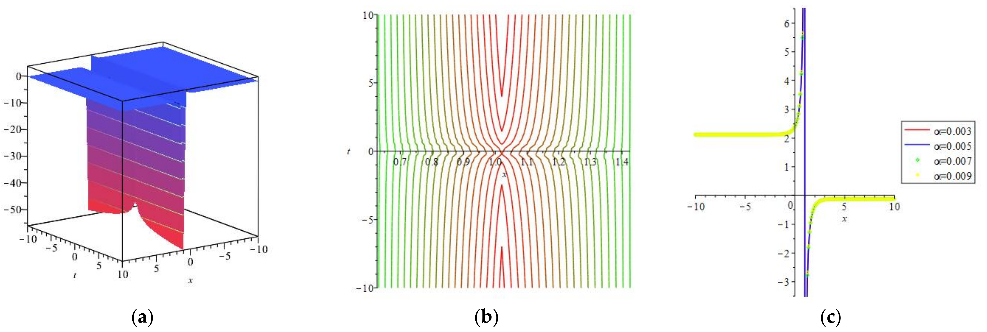
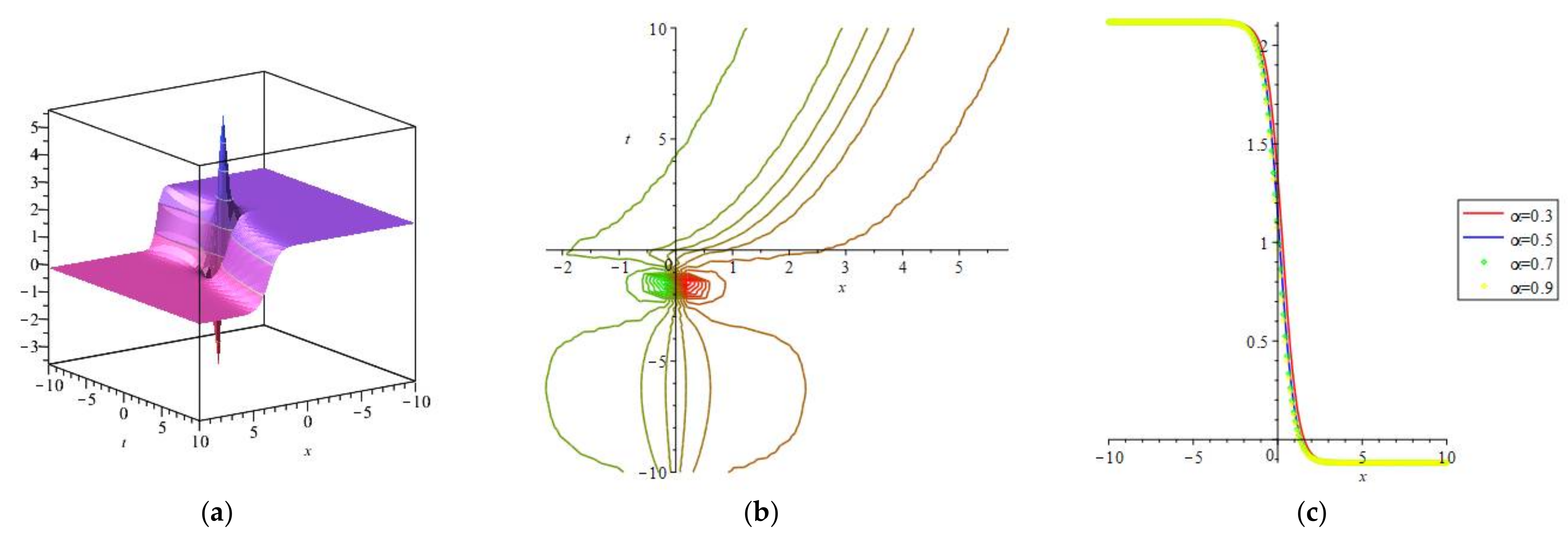
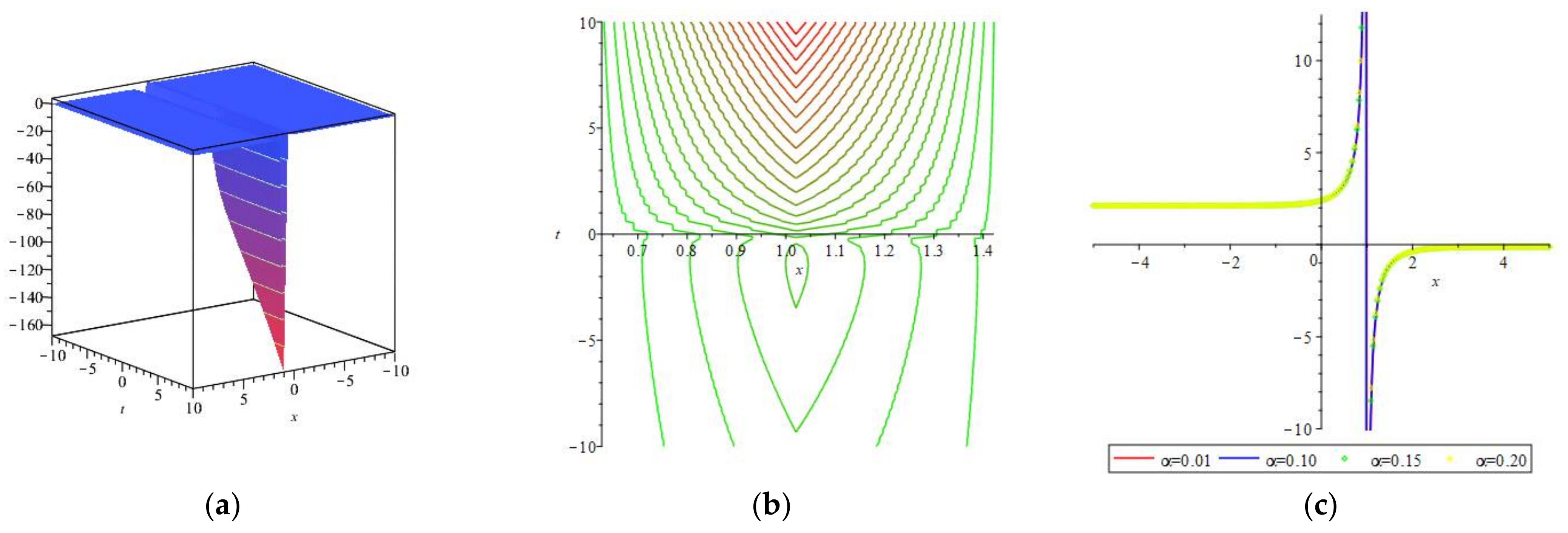
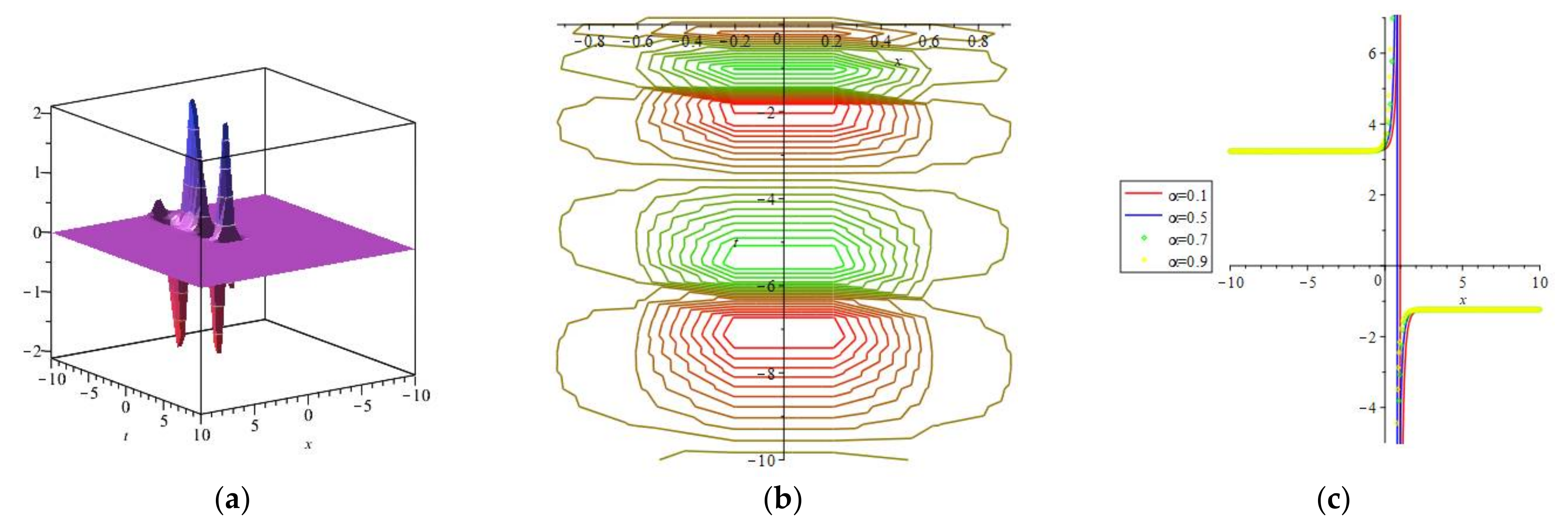
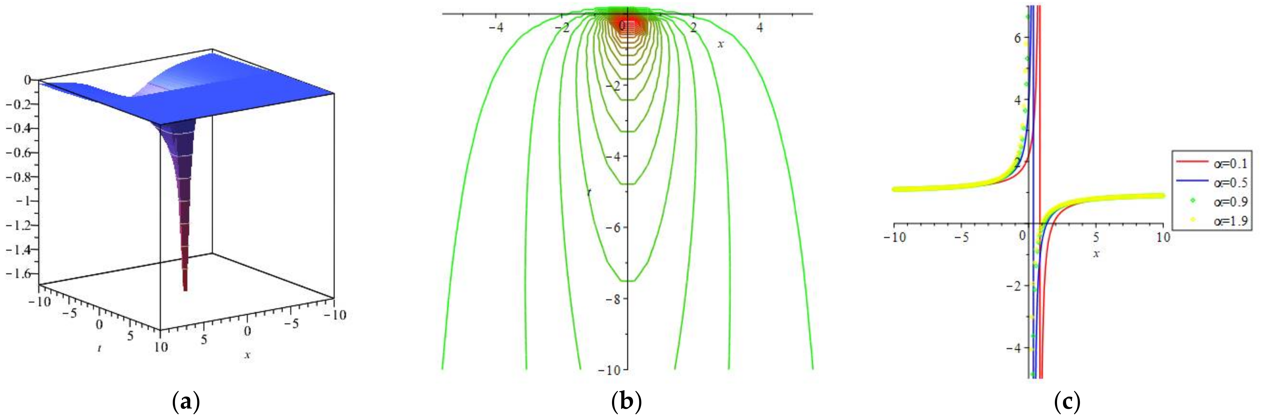
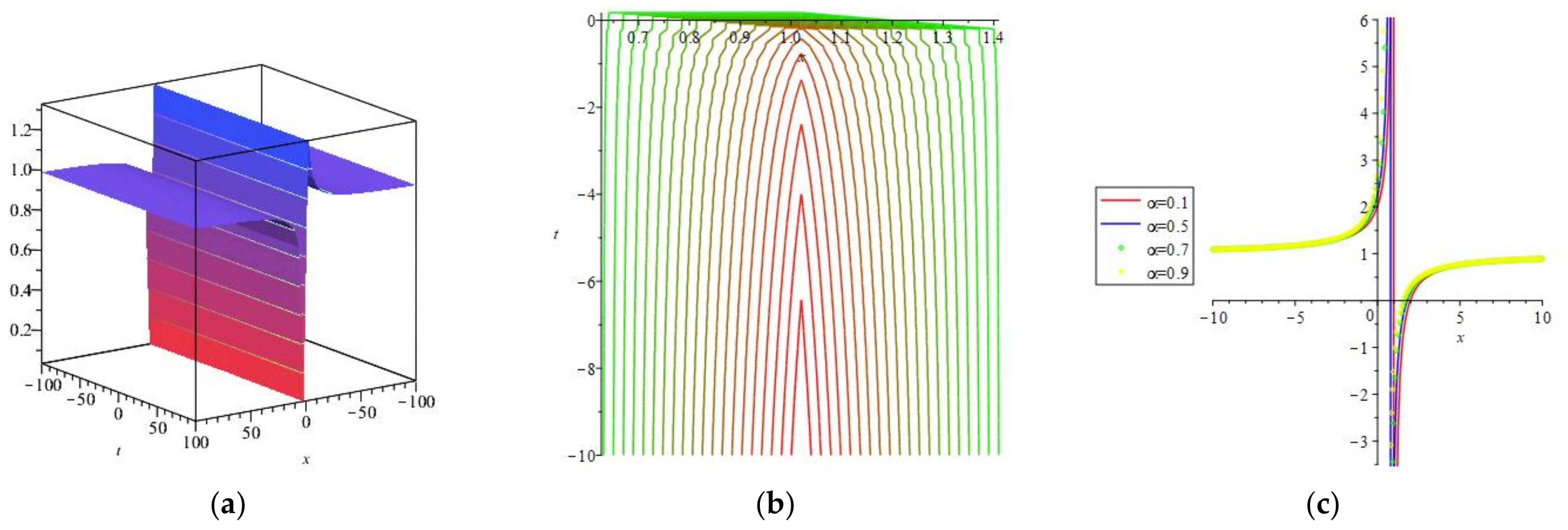
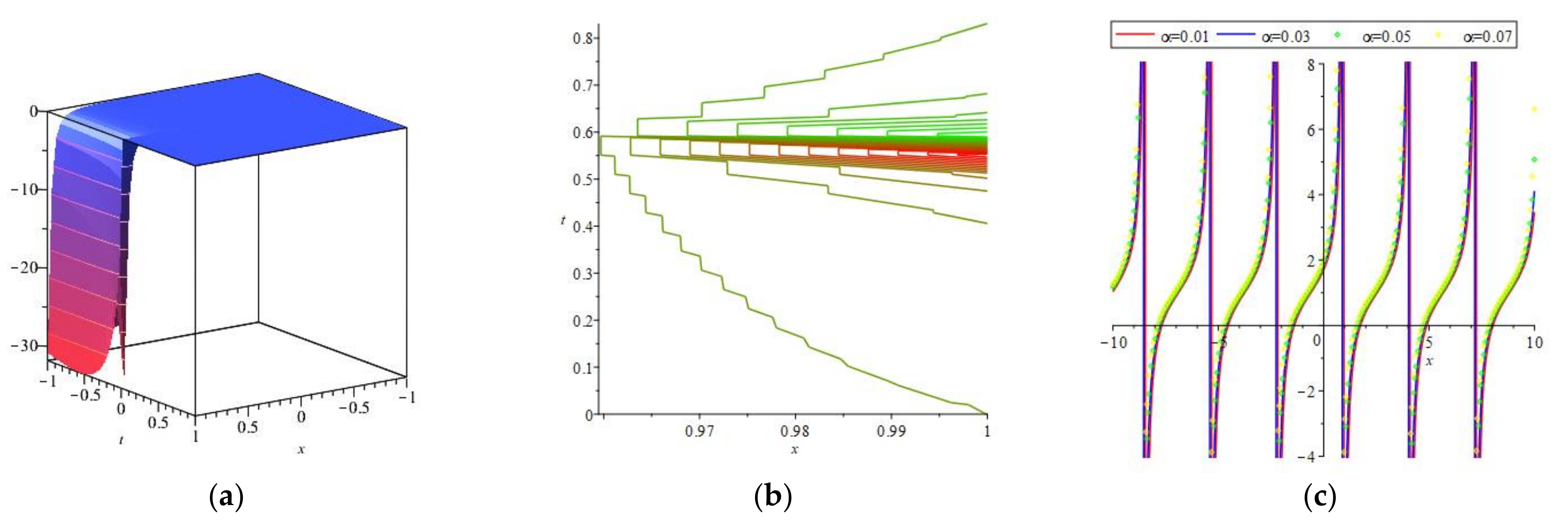
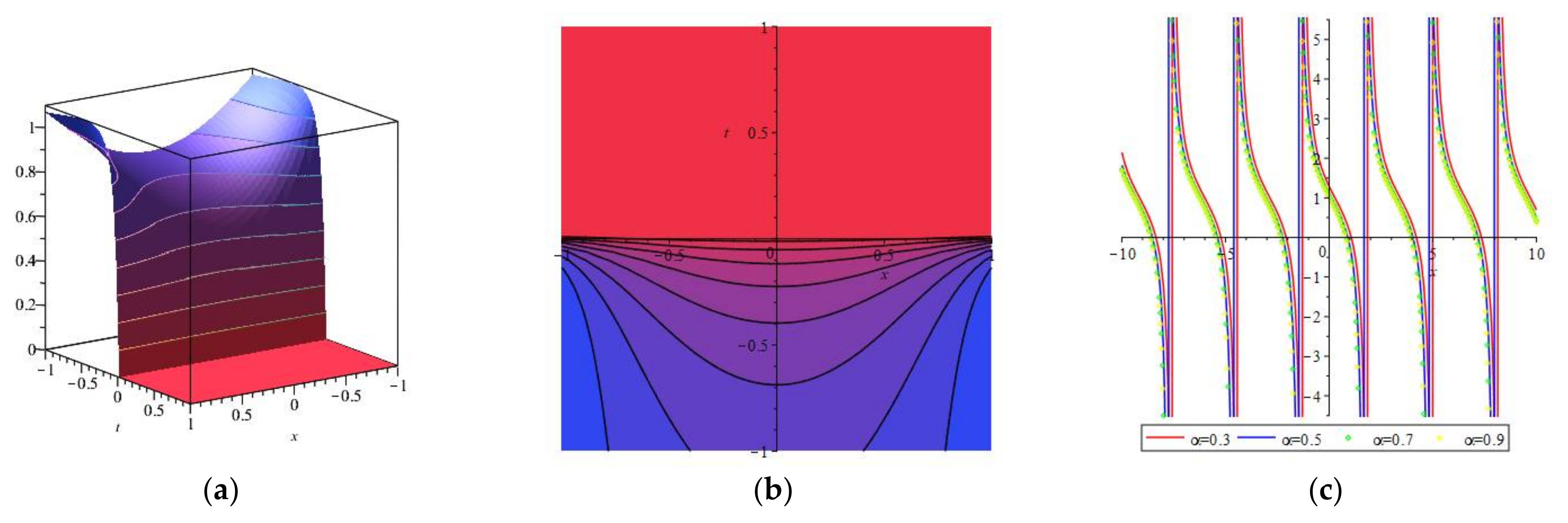
4. Numerical Simulations

Ma et al. [24] introduced a process named the revised (G′/G)-extension approach to look for the FCRWP equation’s exact structures and achieved fifteen results, shown in Section 3. Gunner et al. [37] reported a process named the (G′/G)-extension approach to look for the FCRWP equation’s exact structures and achieved three results. In comparing the two methods, the revised (G′/G)-extension approach provides a more exact answer than the (G′/G)-extension approach. In terms of additional support, the auxiliary model employed in the integral method is different, so the exact structures obtained are also different. Likewise, for any NLFMM, it could be determined that the revised (G′/G)-extension approach is much more straightforward than the other schemes. In this paper, the integrable method is applied to the FCRWP equation for the first time. We confirm that no other author has used the technique on the FCRWP equation. This paper expresses various varieties of exact solutions of the answers for countless values of the constant coefficients. The exact solutions are: dark soliton profiles, singular kink profiles, dark singular soliton profiles, bright and dark lump shapes, periodic wave profiles, etc. Furthermore, we offer a contour graph of the obtained answers, which was created by commencing binary variable tasks. One variable is demonstrated on the horizontal and vertical axes of the contour graph. The functional value exemplifies the color gradient and isolines. The contour graph is a technique used to express a 3D surface on a 2D plane. This kind of graph is broadly implemented in mathematics, physics, as well as engineering, where the contour lines normally represent elevation. We obtained exact solutions like trigonometric, hyperbolic, and rational function answers through the proposed procedure. The solutions to ${\mathrm{ƛ}}_{11}\left(\chi \right)$, ${\mathrm{ƛ}}_{12}\left(\chi \right)$, ${\mathrm{ƛ}}_{21}\left(\chi \right)$, ${\mathrm{ƛ}}_{22}\left(\chi \right)$, ${\mathrm{ƛ}}_{31}\left(\chi \right)$, and ${\mathrm{ƛ}}_{32}\left(\chi \right)$ present as trigonometric function solutions; the solutions of ${\mathrm{ƛ}}_{14}\left(\chi \right)$, ${\mathrm{ƛ}}_{15}\left(\chi \right)$, ${\mathrm{ƛ}}_{24}\left(\chi \right)$, ${\mathrm{ƛ}}_{25}\left(\chi \right)$, ${\mathrm{ƛ}}_{34}\left(\chi \right)$, and ${\mathrm{ƛ}}_{35}\left(\chi \right)$ present as hyperbolic function solutions; and the solutions of ${\mathrm{ƛ}}_{13}\left(\chi \right)$, ${\mathrm{ƛ}}_{23}\left(\chi \right)$, and ${\mathrm{ƛ}}_{33}\left(\chi \right)$ present as trigonometric function solutions. We explain the dynamic performance of the trigonometric function answers of ${\mathrm{ƛ}}_{11}\left(\chi \right)$, ${\mathrm{ƛ}}_{12}\left(\chi \right)$, ${\mathrm{ƛ}}_{22}\left(\chi \right)$, and ${\mathrm{ƛ}}_{31}\left(\chi \right)$, which are illustrated in Figure 1, Figure 2, Figure 3 and Figure 4. In particular, Figure 1, Figure 2, Figure 3 and Figure 4 demonstrate the 3D shape, contour plot, and 2D graph for different values of $\alpha$ for the trigonometric function answers of ${\mathrm{ƛ}}_{11}\left(\chi \right)$, ${\mathrm{ƛ}}_{12}\left(\chi \right)$, ${\mathrm{ƛ}}_{22}\left(\chi \right)$, and ${\mathrm{ƛ}}_{31}\left(\chi \right)$. We explain the dynamic performance of the rational function answers to ${\mathrm{ƛ}}_{23}\left(\chi \right)$ and ${\mathrm{ƛ}}_{33}\left(\chi \right)$, as illustrated in Figure 5 and Figure 6. Figure 5 and Figure 6 demonstrate the 3D shape, contour plot, and 2D graph for different values of $\alpha$ for the rational function answers to ${\mathrm{ƛ}}_{23}\left(\chi \right)$ and ${\mathrm{ƛ}}_{33}\left(\chi \right)$. Finally, we explain the dynamic performance of the trigonometric function answers of ${\mathrm{ƛ}}_{14}\left(\chi \right)$, ${\mathrm{ƛ}}_{15}\left(\chi \right)$, ${\mathrm{ƛ}}_{25}\left(\chi \right)$, and ${\mathrm{ƛ}}_{34}\left(\chi \right)$ in Figure 7, Figure 8, Figure 9 and Figure 10, which depict the 3D shape, contour plot, and 2D graph for different values of $\alpha$ for the trigonometric function answers of ${\mathrm{ƛ}}_{14}\left(\chi \right)$, ${\mathrm{ƛ}}_{15}\left(\chi \right)$, ${\mathrm{ƛ}}_{25}\left(\chi \right)$, and ${\mathrm{ƛ}}_{34}\left(\chi \right)$. The implemented mathematical simulations acknowledge that the answers are of periodic wave shapes and of rational, hyperbolic, and trigonometric categorizations. Furthermore, through observing the construction of the acquired answers, it could be understood that the connecting fractional derivatives of parameter $\alpha$ perform in the formulation of all the answers.

5. Conclusions

In this investigation, we successfully devised a procedure that demonstrates that this system is well-organized and effectively acceptable for finding the exact answers to the FCRWP equation. A wide variety of dynamical behaviors were considered in this study, which presented in well-defined regions of mathematical physics. The most important advantage of this method is that it can more easily reach the solutions than the other analytical schemes for solving NLFMMs. These answers will be valuable for further studies in mathematical physics.

References

1. Alam, M.N.; Seadawy, A.R.; Baleanu, D. Closed-form wave structures of the space-timefractional Hirota–Satsuma coupled KdVequation with nonlinear physical phenomena. Open Phys. 2021, 18, 555–565. [Google Scholar] [CrossRef]
2. Islam, S.; Alam, M.N.; Asad, M.F.A.; Tunc, C. An analytical technique for solving new computational solutions of the modified Zakharov-Kuznetsov equation arising in electrical engineering. J. Appl. Comput. Mech. 2021, 7, 715–726. [Google Scholar]
3. Alam, M.N.; Tunc, C. The new solitary wave structures for the (2 + 1)-dimensional time-fractional Schrodinger equation and the space-time nonlinear conformable fractional Bogoyavlenskii equations. Alex. Eng. J. 2020, 59, 2221–2232. [Google Scholar] [CrossRef]
4. Alam, M.N.; Li, X. New soliton solutions to the nonlinear complex fractional Schrödinger equation and the conformable time-fractional Klein–Gordon equation with quadratic and cubic nonlinearity. Phys. Scr. 2020, 95, 045224. [Google Scholar] [CrossRef]
5. Alam, M.N.; Osman, M.S. New structures for closed-form wave solutions for the dynamical equations model related to the ion sound and Langmuir waves. Commun. Theor. Phys. 2021, 73, 035001. [Google Scholar] [CrossRef]
6. Park, C.; Nuruddeen, R.I.; Ali, K.K.; Muhammad, L.; Osman, M.S.; Baleanu, D. Novel hyperbolic and exponential ansatz methods to the fractional fifth-order Korteweg-de Vries equations. Adv. Differ. Equ. 2020, 2020, 627. [Google Scholar] [CrossRef]
7. Ahmad, H.; Khan, T.A.; Ahmad, I.; Stanimirović, P.S.; Chu, Y.M. A new analyzing technique for nonlinear time fractional Cauchy reaction-diffusion model equations. Results Phys. 2020, 19, 103462. [Google Scholar] [CrossRef]
8. Ahmad, H.; Akgül, A.; Khan, T.A.; Stanimirović, P.S.; Chu, Y.M. New perspective on the conventional solutions of the nonlinear time fractional partial differential equations. Complexity 2020, 2020, 8829017. [Google Scholar] [CrossRef]
9. Osman, M.S.; Rezazadeh, H.; Eslami, M. Traveling wave solutions for (3 + 1) dimensional conformable fractional Zakharov-Kuznetsov equation with power law nonlinearity. Nonlinear Eng. 2019, 8, 559–567. [Google Scholar] [CrossRef]
10. Yepez-Martınez, H.; Gomez-Aguilar, J.F.; Atangana, A. First integral method for non-linear differential equations with conformable derivative. Math. Model. Nat. Phenom. 2018, 13, 14. [Google Scholar] [CrossRef]
11. Aminikhah, H.; Sheikhani, A.H.R.; Rezazadeh, H. Sub-equation method for the fractional regularized long-wave equations with conformable fractional derivatives. Sci. Iran. 2016, 23, 1048–1054. [Google Scholar] [CrossRef] [Green Version]
12. Jiang, J.; Feng, Y.; Li, S. Improved fractional sub-equation method and exact solutions to fractional partial differential equations. J. Funct. Sp. 2020, 2020, 5840920. [Google Scholar]
13. Aslan, E.C.; Inc, M. Optical soliton solutions of the NLSE with quadratic-cubic-hamiltonian perturbations and modulation instability analysis. Optik 2019, 196, 162661. [Google Scholar] [CrossRef]
14. Gurefe, Y. The generalized Kudryashov method for the nonlinear fractional partial differential equations with the beta-derivative. Rev. Mex. Fısica 2020, 66, 771–781. [Google Scholar] [CrossRef]
15. Alam, M.N.; Bonyah, E.; Asad, M.F.A.; Osman, M.S.; Abualnaja, K.M. Stable and functional solutions of the Klein-Fock-Gordon equation with nonlinear physical phenomena. Phys. Scr. 2021. accepted. [Google Scholar] [CrossRef]
16. Tozar, A.; Kurt, A.; Tasbozan, O. New wave solutions of time fractional integrable dispersive wave equation arising in ocean engineering models. Kuwait J. Sci. 2020, 47, 22–33. [Google Scholar]
17. Ismail, G.M.; Rahim, H.R.A.; Aty, A.A.; Kharabsheh, R.; Alharbi, W.; Aty, M.A. An analytical solution for fractional oscillator in a resisting medium. Chaos Solitons Fract. 2020, 130, 109395. [Google Scholar] [CrossRef]
18. Yepez-Martınez, H.; Gomez-Aguilar, J.F. Fractional sub-equation method for Hirota-Satsuma-coupled KdV equation and coupled mKdV equation using the Atangana’s conformable derivative. Waves Random Complex Media 2019, 29, 678–693. [Google Scholar] [CrossRef]
19. Hosseini, K.; Mirzazadeh, M.; Rabiei, F.; Baskonus, H.M.; Yel, G. Dark optical solitons to the Biswas–Arshed equation with high order dispersions and absence of the self-phase modulation. Optik 2020, 209, 164576. [Google Scholar] [CrossRef]
20. Ghanbari, B.; Baleanu, D. New Optical Solutions of the Fractional Gerdjikov-Ivanov Equation with Conformable Derivative. Front. Phys. 2020, 8, 167. [Google Scholar] [CrossRef]
21. Hosseini, K.; Mirzazadeh, M.; Ilie, M.; Radmehr, S. Dynamics of optical solitons in the perturbed Gerdjikov–Ivanov equation. Optik 2020, 206, 164350. [Google Scholar] [CrossRef]
22. Korkmaz, A.; Hepson, O.E.; Hosseini, K.; Rezazadeh, H.; Eslami, M. Sine-gordon expansion method for exact solutions to conformable time fractional equations in RLW-class. J. King Saud Univ. Sci. 2020, 32, 567–574. [Google Scholar] [CrossRef]
23. Hosseini, K.; Mirzazadeh, M.; Vahidi, J.; Asghari, R. Optical wave structures to the Fokas–Lenells equation. Optik 2020, 207, 164450. [Google Scholar] [CrossRef]
24. Ma, X.; Pan, Y.; Chang, L. The modified (G′/G)-expansion method and its applications to KdV equation. Int. J. Nonlinear Sci. 2011, 12, 400–404. [Google Scholar]
25. Miller, K.S.; Ross, B. An Introduction to the Fractional Calculus and Fractional Differential Equations; Wiley: New York, NY, USA, 1993. [Google Scholar]
26. Kilbas, A.A.; Srivastava, H.M.; Trujillo, J.J. Theory and Applications of Fractional Differential Equations; Elsevier: San Diego, CA, USA, 2006. [Google Scholar]
27. Podlubny, I. Fractional Differential Equations; Academic Press: Cambridge, MA, USA, 1999. [Google Scholar]
28. Atangana, A.; Baleanu, D. New fractional derivatives with nonlocal and non-singular kernel: Theory and application to heat transfer model. Therm. Sci. 2016, 20, 763–769. [Google Scholar] [CrossRef] [Green Version]
29. Kumar, A.; Vats, R.K.; Kumar, A.; Chalishajar, D.N. Numerical approach to the controllability of fractional order impulsive differential equations. Demonstr. Math. 2020, 53, 193–207. [Google Scholar] [CrossRef]
30. Caputo, M.; Fabrizio, M. A new definition of fractional derivative without singular kernel. Progr. Fract. Differ. Appl. 2015, 1, 73–85. [Google Scholar] [CrossRef]
31. Harjani, J.; López, B.; Sadarangani, K. Existence and uniqueness of mild solutions for a fractional differential equation under Sturm-Liouville boundary conditions when the data function is of Lipschitzian type. Demonstr. Math. 2020, 53, 167–173. [Google Scholar] [CrossRef]
32. Khalil, R.; Horani, M.A.; Yousef, A.; Sababheh, M. A new definition of fractional derivative. J. Comput. Appl. Math. 2014, 264, 65–70. [Google Scholar] [CrossRef]
33. Atangana, A.; Baleanu, D.; Alsaedi, A. New properties of conformable derivative. Open Math. 2015, 13, 889–898. [Google Scholar] [CrossRef]
34. Jumarie, G. Modified Riemann-Liouville derivative and fractional Taylor series of nondifferentiable functions further results. Comput. Math. Appl. 2006, 51, 1367–1376. [Google Scholar] [CrossRef] [Green Version]
35. Jumarie, G. Table of some basic fractional calculus formulae derived from a modified Riemann-Liouville derivative for non-differentiable functions. Appl. Math. Lett. 2009, 22, 378–385. [Google Scholar] [CrossRef]
36. Ganji, Z.; Ganji, D.; Ganji, A.D.; Rostamian, M. Analytical solution of time-fractional Navier–Stokes equation in polar coordinate by homotopy perturbation method. Numer. Methods Partial Differ. Equ. 2010, 26, 117–124. [Google Scholar] [CrossRef]
37. Gunera, O.; Bekir, A.; Ünsal, Ö. Two reliable methods for solving the time fractional Clannish Random Walker’s Parabolic equation. Optik 2016, 127, 9571–9577. [Google Scholar] [CrossRef]
Figure 1. The graphical representation of the solution ƛ 11 χ : (a) 3D shape, (b) contour plot, and (c) 2D graph.
Mathematics 09 00801 g001
Figure 2. The graphical representation of the solution ƛ 12 χ : (a) 3D shape, (b) contour plot, and (c) 2D graph.
Mathematics 09 00801 g002
Figure 3. The graphical representation of the solution ƛ 22 χ : (a) 3D shape, (b) contour plot, and (c) 2D graph.
Mathematics 09 00801 g003
Figure 4. The graphical representation of the solution ƛ 31 χ : (a) 3D shape, (b) contour plot, and (c) 2D graph.
Mathematics 09 00801 g004
Figure 5. The graphical representation of the solution ƛ 23 χ : (a) 3D shape, (b) contour plot, and (c) 2D graph.
Mathematics 09 00801 g005
Figure 6. The graphical representation of the solution ƛ 33 χ : (a) 3D shape, (b) contour plot, and (c) 2D graph.
Mathematics 09 00801 g006
Figure 7. The graphical representation of the solution ƛ 14 χ : (a) 3D shape, (b) contour plot, and (c) 2D graph
Mathematics 09 00801 g007
Figure 8. The graphical representation of the solution ƛ 15 χ : (a) 3D shape, (b) contour plot, and (c) 2D graph.
Mathematics 09 00801 g008
Figure 9. The graphical representation of the solution ƛ 25 χ : (a) 3D shape, (b) contour plot, and (c) 2D graph.
Mathematics 09 00801 g009
Figure 10. The graphical representation of the solution ƛ 34 χ : (a) 3D shape, (b) contour plot, and (c) 2D graph.
Mathematics 09 00801 g010
Publisher’s Note: MDPI stays neutral with regard to jurisdictional claims in published maps and institutional affiliations.