
Optimization of the ANNs Predictive Capability Using the Taguchi Approach: A Case Study

Abstract
1. Introduction
2. Materials and Methods
2.1. The Multi-Layer Perceptron (MLP) Model
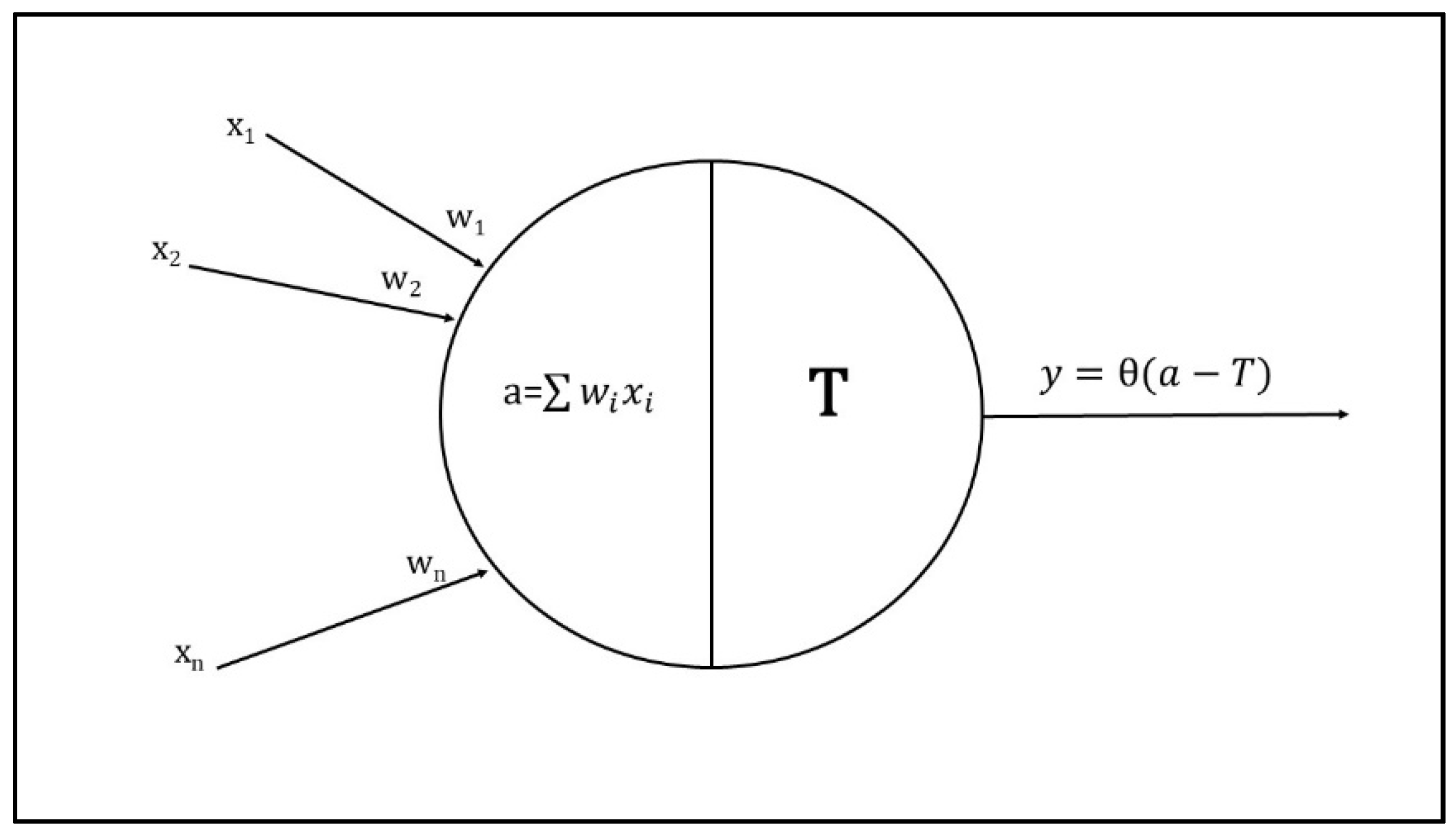
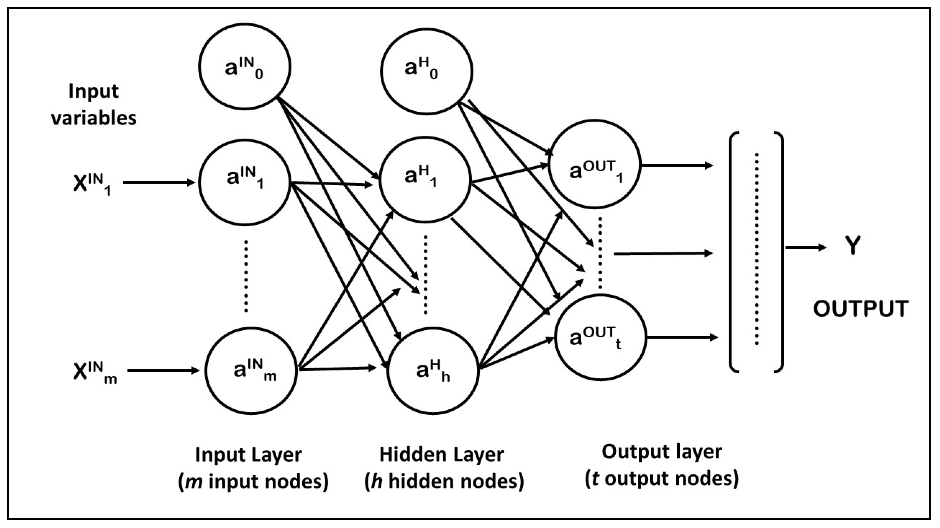
2.1.1. Neurons and Layers
2.1.2. Activation Function
2.1.3. The Training Process and Pre-Treatment of Data
- Training phase, to find the weights that represent the relationship between ANN inputs and outputs.
- Testing phase, to optimize the weights and to estimate model accuracy by error indicators.
2.1.4. The Training Cycles and Network Performance
- (a)
- Coefficient of Determination (R2)
- (b)
- Mean Absolute Error (MAE)
- (c)
- Root Mean Squared Error (RMSE)
2.1.5. The Taguchi Design of Experiments Method
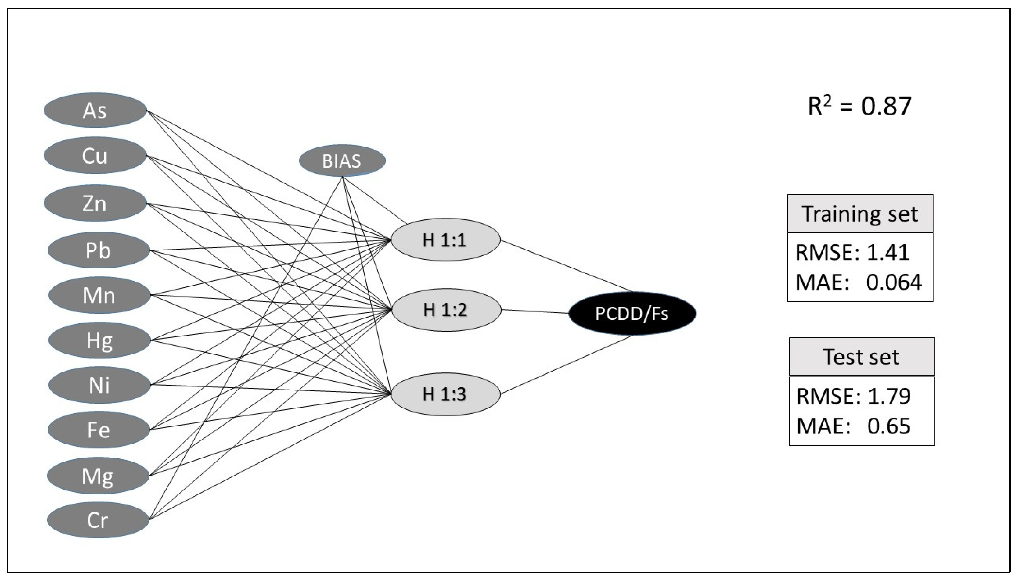
2.2. A Case Study: Use of Artificial Neural Networks to Evaluate Organic and Inorganic Contamination in Agricultural Soils
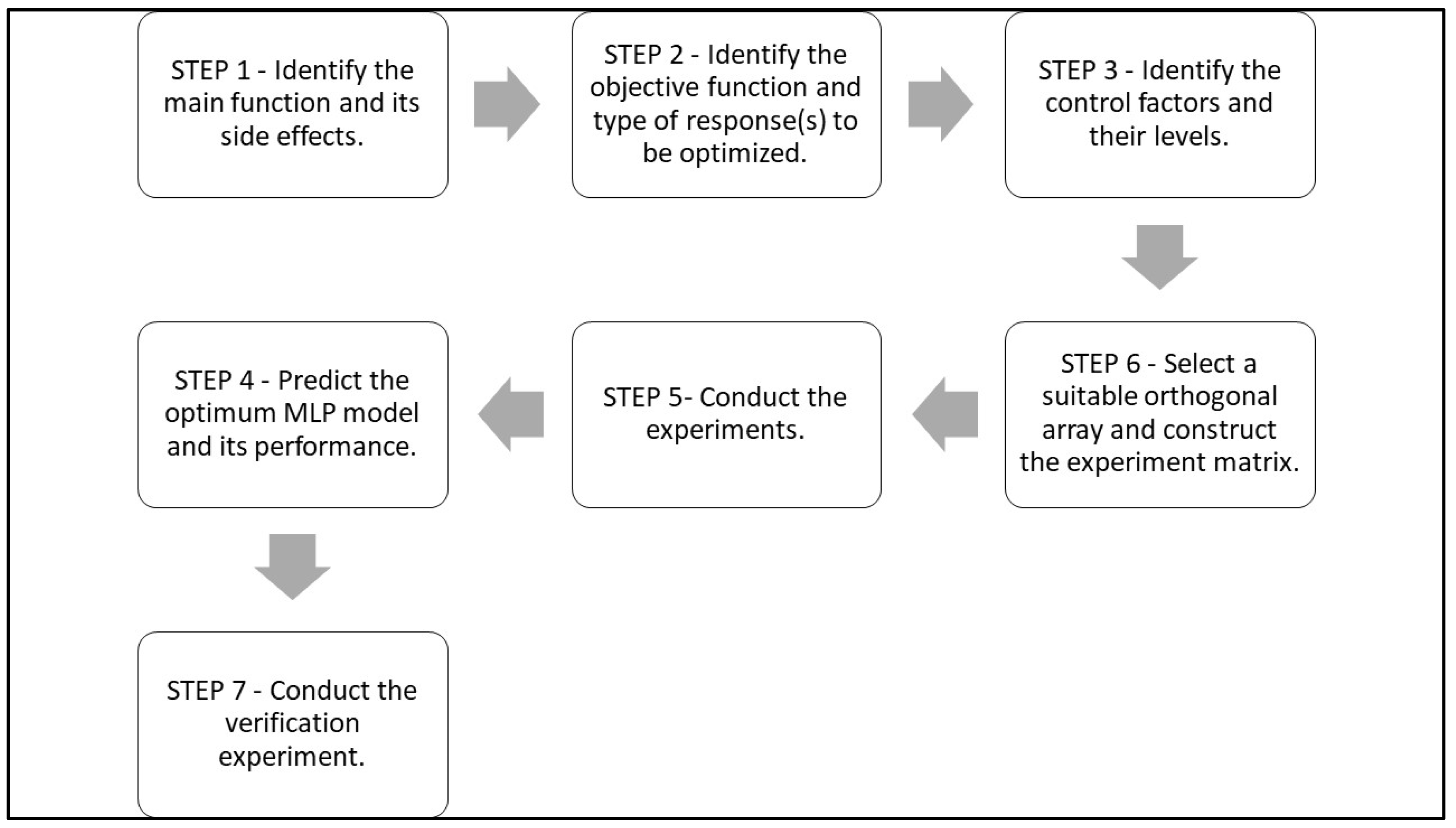
The Taguchi Design Steps to Optimize the Predictive Xapability of ANNs
3. Results
3.1. Step 1. Identify the Main Function and Its Side Effects
3.2. Step 2. Identify the Objective Function and Type of Response(s) to Be Optimized
3.3. Step 3. Identify the Control Factors and Their Levels
- Number of samples. The experiment can detect the minimum number of sample units sufficient for the network to learn. In a 64-sample database, three levels of this factor have been fixed: 10, 30, and 50 units.
- Input scaling rule. Two levels are corresponding to the different criteria to scale input data (§ 2.3):
- (a)
- normalization, using the formula
- (b)
- standardization, using the formula
- Training rate (%): three levels of percentage have been considered for computing the size of the training set (test set): 60% (40%), 70% (30%), and 80% (20%).
- Activation function of hidden and output nodes: as mentioned above (§ 2.2), two levels have been chosen for the activation function of the hidden nodes (sigmoid and hyperbolic tangent), and three levels for the activation function of output nodes (identity function, sigmoid, and hyperbolic tangent).
- Number of hidden layers: to determine if a deep network has better predictive performance, two levels of this factor have been considered: one or two hidden layers, as allowed by Neural Network function in IBM-SPSS.
- Epochs. The training process duration has been set to three levels: 10, 10,000, and 60,000 epochs.
3.4. Step 4. Select a Suitable Orthogonal Array and Construct the Experiment Matrix
3.5. Step 5. Conduct the Experiments
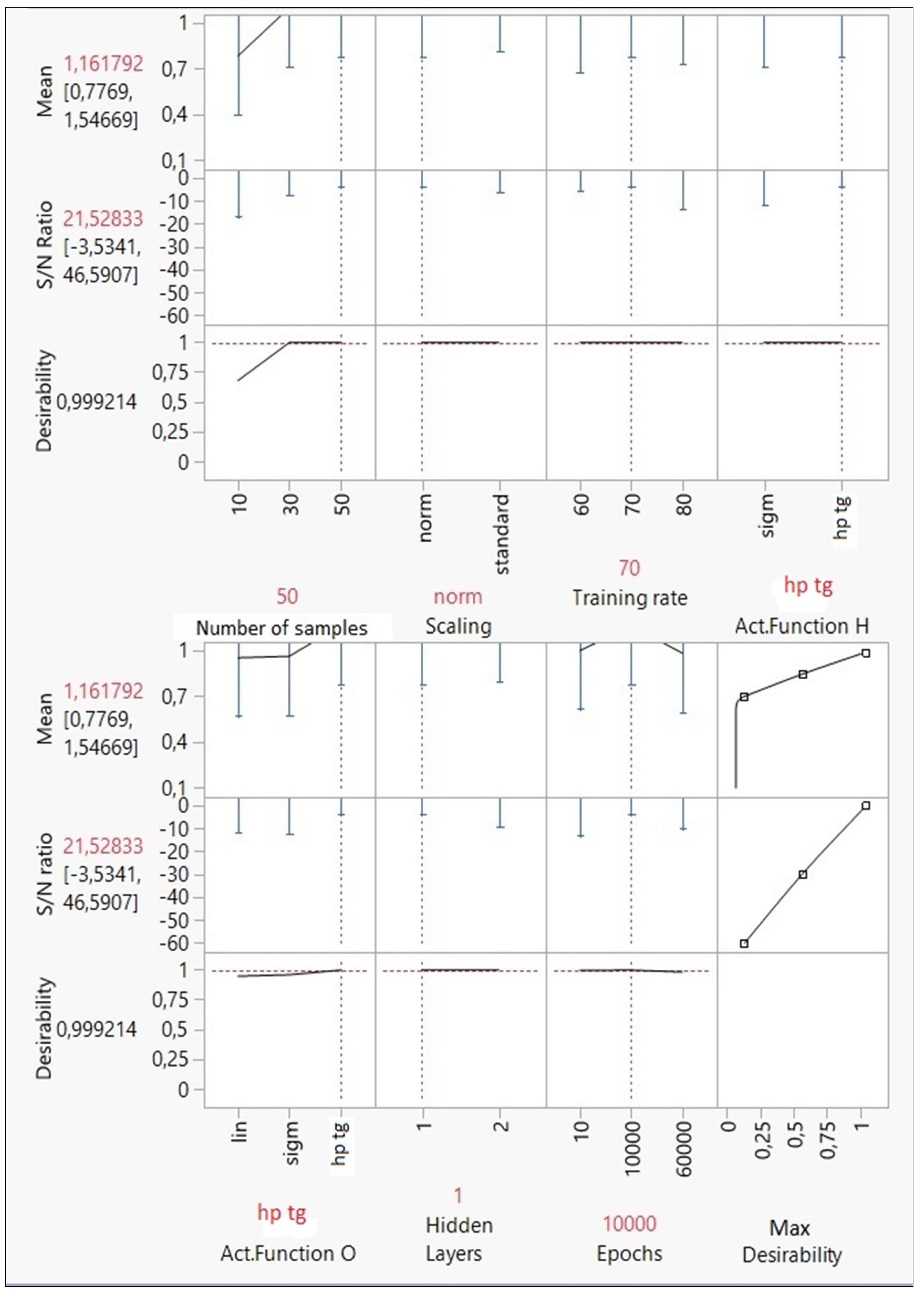
3.6. Step 6. Predict the Optimum MLP Model and Its Performance
- Number of samples: at least 50 samples are required to obtain an optimal model. Thus, a small number of units could cause unbiased predictions.
- Input scaling rule: the normalization of input variables produces better results than the standardization rule.
- Training rate (%): in an optimal MLP model, the training set must consider 70% of database units. Thus, the test set represents the remaining 30%.
- Activation function of hidden and output nodes: the best activation function is the hyperbolic tangent for both hidden and output nodes.
- Number of hidden layers: according to Taguchi’s design, a deep network is not the best solution for this analysis; one hidden layer has been more than enough to optimize the forecasts.
- Epochs: the model accuracy has been determined in 10,000 epochs.
3.7. Step 7. Conduct the Verification Experiment
4. Conclusions
Author Contributions
Funding
Institutional Review Board Statement
Informed Consent Statement
Data Availability Statement
Conflicts of Interest
References
- Gardner, M.W.; Dorling, S.R. Artificial neural networks (the multi-layer perceptron)—A review of applications in the atmospheric sciences. Atmos. Environ. 1998, 32, 2627–2636. [Google Scholar] [CrossRef]
- Gomes-Ramos, E.; Venegas-Martinez, F. A Review of Artificial Neural Networks: How Well Do They Perform in Forecasting Time Series? Analìtika 2013, 6, 7–15. [Google Scholar]
- Haykin, S. Neural Networks a Comprehensive Foundation; Prentice Hall PTR: Upper Saddle River, NJ, USA, 1994. [Google Scholar]
- Bishop, C.M. Neural Networks for Pattern Recognition, 3rd ed.; Oxford University Press: Oxford, UK, 1995. [Google Scholar]
- Mc Culloch, W.S.; Pitts, W. A logical calculus of the ideas immanent in nervous activity. Bull. Math. Biol. 1943, 5, 115–133. [Google Scholar]
- Agatonovic-Kustrin, S.; Beresford, R. Basic concepts of artificial neural network (ANN) modeling and its application in pharmaceutical research. J. Pharm. Biomed. Anal. 2000, 22, 717–727. [Google Scholar] [CrossRef]
- Karlik, B.; Vehbi Olgac, A.V. Performance Analysis of Various Activation Functions in Generalized MLP Architectures of Neural Networks. Int. J. Artif. Intell. Expert Syst. 2011, 1, 111–122. [Google Scholar]
- Maier, H.R.; Dandy, G.C. The effect of internal parameters and geometry on the performance of back-propagation neural networks: An empirical study. Environ. Model. Softw. 1998, 13, 193–209. [Google Scholar] [CrossRef]
- Maier, H.R.; Dandy, G.C. Understanding the behaviour and optimising the performance of back-propagation neural networks: An empirical study. Environ. Model. Softw. 1998, 13, 179–191. [Google Scholar] [CrossRef]
- Ross, J.P. Taguchi Techniques for Quality Engineering; McGraw-Hill: New York, NY, USA, 1996. [Google Scholar]
- Wang, S.H.; Wu, X.; Zhang, Y.D.; Tang, C.; Zhang, X. Diagnosis of COVID-19 by Wavelet Renyi Entropy and Three-Segment Biogeography-Based Optimization. Int. J. Comput. Int. Syst. 2020, 13, 1332–1344. [Google Scholar] [CrossRef]
- Zhang, Y.D.; Sui, Y.; Sun, J.; Zhao, G.; Qian, P. Cat Swarm Optimization applied to alcohol use disorder identification. Multimed. Tools Appl. 2018, 77, 22875–22896. [Google Scholar] [CrossRef]
- Bonfitto, A.; Feraco, S.; Tonoli, A.; Amati, N.; Monti, F. Estimation accuracy and computational cost analysis of artificial neural networks for state of charge estimation in lithium batteries. Batteries 2019, 5, 47. [Google Scholar] [CrossRef]
- Dinesh Kumar, D.; Gupta, A.K.; Chandna, P.; Pal, M. Optimization of neural network parameters using Grey–Taguchi methodology for manufacturing process applications. J. Mech. Eng. Sci. 2015, 229, 2651–2664. [Google Scholar] [CrossRef]
- Ma, L.; Khorasani, K. A new strategy for adaptively constructing multi-layer feed-forward neural networks. Neurocomputing 2003, 51, 361–385. [Google Scholar] [CrossRef]
- Kwon, Y.K.; Moon, B.R. A hybrid neurogenetic approach for stock forecasting. IEEE Trans. Neural Netw. 2007, 18, 851–864. [Google Scholar] [CrossRef]
- Bebis, G.; Georgiopoulos, M.; Kasparis, T. Coupling weight elimination with genetic algorithms to reduce network size and preserve generalization. Neurocomputing 1997, 17, 167–194. [Google Scholar] [CrossRef]
- Benardos, P.G.; Vosniakos, G.C. Optimizing feed-forward artificial neural network architecture. Eng. Appl. Artif. Intell. 2007, 20, 365–382. [Google Scholar] [CrossRef]
- Marijke, K. Genetic Algorithms, Anoverview. 2002. Available online: http://www.meteck.org/gaover.html (accessed on 31 March 2021).
- Arifovic, J.; Gencay, R. Using genetic algorithms to select architecture of a feed-forward artificial neural network. Physica 2001, 289, 574–594. [Google Scholar] [CrossRef]
- Yang, J.L.; Chen, J.C. A Systematic Approach for Identifying Optimum Surface Roughness Performance in End-Milling Operations. J. Ind. Technol. 2001, 17, 2–8. [Google Scholar]
- Lin, C.; Li, Y.-C.; Lin, H.-Y. Using Convolutional Neural Networks Based on a Taguchi Method for Face Gender Recognition. Electronics 2020, 9, 1227. [Google Scholar] [CrossRef]
- Tabassum, M.; Mathew, K. A Genetic Algorithm Analysis towards Optimization solutions. Int. J. Digit. Inf. Wirel. Commun. 2014, 4, 124–142. [Google Scholar] [CrossRef]
- Larochelle, H.; Jerome, Y.B.; Lamblin, L.P. Exploring Strategies for Training Deep Neural Networks. J. Mach. Learn. Res. 2009, 1, 1–40. [Google Scholar]
- Li, L. Introduction to Multilayer Neural Networks with TensorFlow’s Keras. API. Available online: https://towardsdatascience.com/ (accessed on 31 March 2021).
- Hornik, K. Approximation capabilities of multi-layer feed-forward networks. Neural Netw. 1991, 4, 251–257. [Google Scholar] [CrossRef]
- Schmidhuber, J. Deep Learning in Neural Networks: An Overview. Neural Netw. 2015, 61, 85–117. [Google Scholar] [CrossRef] [PubMed]
- Sutton, R.S. Two problems with back-propagation and other steepest-descent learning procedures for networks. In Proceedings of the Eighth Annual Conference of the Cognitive Science Society, Amherst, MA, USA, 15–17 August 1986; pp. 823–831. [Google Scholar]
- Ghaffari, A.; Abdollahi, H.; Khoshayand, M.R.; Soltani Bozchalooi, I.; Dadgar, A.; Rafiee-Tehrani, M. Performance comparison of neural network training algorithms in modeling of bimodal drug delivery. Int. J. Pharm. 2006, 11, 126–138. [Google Scholar] [CrossRef] [PubMed]
- Erb, R.J. Introduction to back-propagation neural network computation. Pharm. Res. 1993, 10, 165–170. [Google Scholar] [CrossRef] [PubMed]
- Leitch, G.; Tanner, J.E. Economic Forecast Evaluation: Prots Versus the Conventional Error Measures. Am. Econ. Rev. 1991, 81, 580–590. [Google Scholar]
- Kuroe, Y.; Yoshid, M.; Mori, T. On Activation Functions for Complex-Valued Neural Networks. In ICANN/ICONIP 2003 Lecture Notes in Computer Science; Springer: Berlin/Heidelberg, Germany, 2003; Volume 2714. [Google Scholar]
- Shmueli, G.; Patel, N.R.; Bruce, P.C. Data Mining for Business Analytics: Concepts, Techniques, and Applications with JMP Pro; John Wiley & Sons Inc.: Hoboken, NJ, USA, 2016. [Google Scholar]
- Musumeci, F.; Rottondi, C.; Nag, A.; Macaluso, I.; Zibar, D.; Ruffini, M.; Tornatore, M. Survey on application of machine learning techniques in optical networks. IEEE Commun. Surv. Tutor. 2018, 1–27. [Google Scholar]
- Demuth, H.; Beale, M.; Hagan, M. 2008; Neural Network ToolboxTM6. User’s Guide MathWorks 2008, 9, 259–265. [Google Scholar]
- Shahin, M.A.; Maier, H.R.; Jaksa, M.B. Data division for developing neural networks applied to geotechnical engineering. J. Comput. Civ. Eng. ASCE 2004, 18, 105–114. [Google Scholar] [CrossRef]
- Gallo, C. Artificial Neural Networks Tutorial. In Enciclopedia of Information, Science and Technology, 3rd ed.; MEHDI Khosrow-Pour Information Resources Management Association: Washington, DC, USA, 2015; pp. 179–189. [Google Scholar]
- Kotsiantis, S.B.; Kanellopoulos, D.; Pintelas, P.E. Data Pre-processing for Supervised Learning. CompSci 2006, 1, 1306–4428. [Google Scholar]
- Shanker, M.; Hu, M.Y.; Hung, M.S. Effect of data standardization on neural network training. Omega 1996, 24, 385–397. [Google Scholar] [CrossRef]
- Mjalli, F.S.; Al-Asheh, S.; Alfadala, H.E. Use of artificial neural network black-box modeling for the prediction of wastewater treatment plants performance. J. Environ. Manag. 2007, 83, 329–338. [Google Scholar] [CrossRef]
- Hush, D.; Horne, B.G. Progress in supervised neural networks. IEEE Signal Process. 1993, 10, 8–39. [Google Scholar] [CrossRef]
- Hornik, K.; Stinchcombe, M.; White, H. Multilayer Feedforward Networks are Universal Approximators. Neural Netw. 1989, 2, 359–366. [Google Scholar] [CrossRef]
- Twomey, J.M.; Smith, A.E. Performance Measures, Consistency and Power for Artificial Neural Network Models. Mathl. Comput. Model. 1995, 21, 243–258. [Google Scholar] [CrossRef]
- Afan, H.; El-Shafie, A.; Yaseen, Z.; Hameed, M.; Wan Mohtar, H.; Hussain, A. ANN Based Sediment Prediction Model Utilizing Different Input Scenarios. Water Resour. Manag. 2015, 29. [Google Scholar] [CrossRef]
- Chaloulakou, A.; Saisana, M.; Spyrellis, N. Comparative assessment of neural networks and regression models for forecasting summertime ozone in Athens. Sci. Total Environ. 2003, 313, 1–13. [Google Scholar] [CrossRef]
- Nalbant, M.; Gökkaya, H.; Sur, G. Application of Taguchi method in the optimization of cutting parameters for surface roughness in turning. Mater. Des. 2007, 28, 1379–1385. [Google Scholar] [CrossRef]
- Antony, J. Fractional Factorial Designs in Design of Experiments for Engineers and Scientists, 2nd ed.; Elsevier Insights: London, UK, 2014; pp. 87–112. [Google Scholar]
- Bonelli, M.G.; Ferrini, M.; Manni, A. Artificial neural networks to evaluate organic and inorganic contamination in agricultural soils. Chemosphere 2017, 186, 124–131. [Google Scholar] [CrossRef]
- IBM SPSS Neural Networks 25. Available online: https://www.ibm.com/downloads/cas/JPKAPO4L (accessed on 31 March 2021).
- Charan Kumar, G.; Varalakshmi, M.; Ankita, T.; Rajyalakshmi, K. Modified Taguchi Approach for optimizing the process parameter using the fictitious parameter. J. Phys.Conf. Ser. 2019, 1344, 1–11. [Google Scholar] [CrossRef]
- Fratilia, D.; Caizar, C. Application of Taguchi method to selection of optimal lubrication and cutting conditions in face milling of AlMg3. J. Clean. Prod. 2011, 19, 640–645. [Google Scholar] [CrossRef]
- Sharma, N.; Ragsdell, K. Quality Loss Function—Common Methodology for Nominal-The-Best, Smaller-The-Better, and Larger-The-Better Cases; SAE Technical Papers; SAE International: Warrendale, PA, USA, 2007. [Google Scholar] [CrossRef]
- Antony, J. Multi-response optimization in industrial experiments using Taguchi’s quality loss function and principal component analysis. Qual. Reliab. Engng. Int. 2000, 16, 3–8. [Google Scholar] [CrossRef]
- Phadke, M.S. Quality Engineering Using Robust Design; Prentice Hall: Englewood Cliffs, NJ, USA, 1989. [Google Scholar]
- John, B. Application of desirability function for optimizing the performance characteristics of carbonitrided bushes. Int. J. Ind. Eng. Comput. 2013, 4, 305–314. [Google Scholar] [CrossRef]
- Derringer, G. A balancing act: Optimising product’s properties. Qual. Prog. 1994, 27, 51–58. [Google Scholar]
- Subrahmanyam, A.; Maheswara Rao, C.; Naga Raju, B. Taguchi based desirability function analysis for the optimization of multiple performance characteristics. IJMTER 2018, 5, 168–175. [Google Scholar]


| Factor | Levels | ||
|---|---|---|---|
| Number of samples | 10 | 30 | 50 |
| Input scaling | normalized; standardized | ||
| Training rate (%) | 60 | 70 | 80 |
| Act. Function H | Sigmoid; Hyperbolic; tangent | ||
| Act. Function O | identity | sigmoid | hyp.tangent |
| n. Hidden Layers | 1 | - | 2 |
| Epochs | 10 | 10,000 | 60,000 |
| Factor | Number of Level (ni) | Degrees of Freedom (ni) −1 |
|---|---|---|
| Mean value | - | 1 |
| Number of samples | 3 | 2 |
| Input scaling | 2 | 1 |
| Training rate (%) | 3 | 2 |
| Act. Function H | 2 | 1 |
| Act. Function O | 3 | 2 |
| n. Hidden Layers | 2 | 1 |
| Epochs | 3 | 2 |
| OA | Number of Samples | Input Scaling | Training Rate (%) | Act. Function H | Act. Function O | n. Hidden Layers | Epochs |
|---|---|---|---|---|---|---|---|
| L1 | 10 | norm | 60 | sigm | lin | 1 | 10 |
| L2 | 30 | norm | 70 | sigm | hp tg | 1 | 10,000 |
| L3 | 50 | norm | 80 | sigm | sigm | 1 | 60,000 |
| L4 | 10 | norm | 80 | hp tg | hp tg | 2 | 10,000 |
| L5 | 30 | norm | 60 | hp tg | sigm | 2 | 60,000 |
| L6 | 50 | norm | 70 | hp tg | lin | 2 | 10 |
| L7 | 10 | standard | 80 | sigm | sigm | 2 | 10 |
| L8 | 30 | standard | 60 | sigm | lin | 2 | 10,000 |
| L9 | 50 | standard | 70 | sigm | hp tg | 2 | 60,000 |
| L10 | 10 | standard | 70 | hp tg | lin | 1 | 60,000 |
| L11 | 30 | standard | 80 | hp tg | hp tg | 1 | 10 |
| L12 | 50 | standard | 60 | hp tg | sigm | 1 | 10,000 |
| OA | R21 | R22 | Mean | S/N Ratio |
|---|---|---|---|---|
| L1 | 0.123 | 0.347 | 0.235 | −15.705 |
| L2 | 0.914 | 0.919 | 0.916 | −0.757 |
| L3 | 0.914 | 0.845 | 0.879 | −1.135 |
| L4 | 0.935 | 0.803 | 0.869 | −1.295 |
| L5 | 0.524 | 0.709 | 0.616 | −4.496 |
| L6 | 0.793 | 0.91 | 0.851 | −1.458 |
| L7 | 0.002 | 0.399 | 0.200 | −50.969 |
| L8 | 0.955 | 0.91 | 0.932 | −0.615 |
| L9 | 0.912 | 0.899 | 0.905 | −0.863 |
| L10 | 0.584 | 0.186 | 0.385 | −12.019 |
| L11 | 0.903 | 0.949 | 0.926 | −0.676 |
| L12 | 0.86 | 0.549 | 0.704 | −3.683 |
| Number of Samples | Input Scaling | Training Rate (%) | Act. Function H | Act. Function O | n. Hidden Layers | Epochs |
|---|---|---|---|---|---|---|
| 50 | norm | 70 | hp tg | hp tg | 1 | 10,000 |
| Network Features | MLPdef1 | MLPdef2 | MLPopt |
|---|---|---|---|
| Number of samples | 64 | 50 | 50 |
| Scaling | standard | standard | norm |
| Training rate | 70 | 70 | 70 |
| Act. FunctionH | tg hp | tg hp | tg hp |
| Act. FunctionO | lin | lin | tg hp |
| Hidden layer | 1 | 1 | 1 |
| Epochs | 10 | 10 | 10,000 |
| Rsquare | 0.87 | 0.63 | 0.93 |
| RMSEtraining | 1.41 | 1.683 | 0.129 |
| RMSEtest | 1.788 | 30.319 | 0.025 |
| MAEtraining | 0.064 | 0.102 | 0.025 |
| MAEtest | 0.65 | 0.488 | 0.691 |
Publisher’s Note: MDPI stays neutral with regard to jurisdictional claims in published maps and institutional affiliations. |
© 2021 by the authors. Licensee MDPI, Basel, Switzerland. This article is an open access article distributed under the terms and conditions of the Creative Commons Attribution (CC BY) license (https://creativecommons.org/licenses/by/4.0/).
Share and Cite
Manni, A.; Saviano, G.; Bonelli, M.G. Optimization of the ANNs Predictive Capability Using the Taguchi Approach: A Case Study. Mathematics 2021, 9, 766. https://doi.org/10.3390/math9070766
Manni A, Saviano G, Bonelli MG. Optimization of the ANNs Predictive Capability Using the Taguchi Approach: A Case Study. Mathematics. 2021; 9(7):766. https://doi.org/10.3390/math9070766
Chicago/Turabian StyleManni, Andrea, Giovanna Saviano, and Maria Grazia Bonelli. 2021. "Optimization of the ANNs Predictive Capability Using the Taguchi Approach: A Case Study" Mathematics 9, no. 7: 766. https://doi.org/10.3390/math9070766
APA StyleManni, A., Saviano, G., & Bonelli, M. G. (2021). Optimization of the ANNs Predictive Capability Using the Taguchi Approach: A Case Study. Mathematics, 9(7), 766. https://doi.org/10.3390/math9070766