Weighted Homology of Bi-Structures over Certain Discrete Valuation Rings

Abstract

An RNA bi-structure is a pair of RNA secondary structures that are considered as arc-diagrams. We present a novel weighted homology theory for RNA bi-structures, which was obtained through the intersections of loops. The weighted homology of the intersection complex X features a new boundary operator and is formulated over a discrete valuation ring, R. We establish basic properties of the weighted complex and show how to deform it in order to eliminate any 3-simplices. We connect the simplicial homology, $H_i(X)$, and weighted homology, $H_{i,R}(X)$, in two ways: first, via chain maps, and second, via the relative homology. We compute $H_{0,R}(X)$ by means of a recursive contraction procedure on a weighted spanning tree and $H_{1,R}(X)$ via an inflation map, by which the simplicial homology of the 1-skeleton allows us to determine the weighted homology $H_{1,R}(X)$. The homology module $H_{2,R}(X)$ is naturally obtained from $H_2(X)$ via chain maps. Furthermore, we show that all weighted homology modules $H_{i,R}(X)$ are trivial for $i>2$. The invariant factors of our structure theorems, as well as the weighted Whitehead moves facilitating the removal of filled tetrahedra, are given a combinatorial interpretation. The weighted homology of bi-structures augments the simplicial counterpart by introducing novel torsion submodules and preserving the free submodules that appear in the simplicial homology.

1. Introduction

This paper is concerned with the weighted homology of the nerve complex of RNA bi-structures [1]. The weighted nerve complex of such bi-structures provides a framework for studying the computational complexity of algorithms for identifying sequences that are thermodynamically stable with respect to a given bi-structure. Such sequences hold the key for evolutionary optimization [2].

The weighted homology introduced here augments the simplicial homology by making the weights of the simplices an integral part of the theory. In our situation, these weights encode the cardinality of intersections of loops in a bi-structure. Along the lines of [3], the notion of a weighted complex is introduced. Differently from [3], the weights of simplices in this paper are taken from a discrete valuation ring that contains a copy of the integers as units and in which the weight of a simplex divides the weight of its faces.

1.1. Background

RNA sequences are linear, single-stranded sequences composed of the bases A,U,G, and C. In contrast to double-stranded DNA, RNA sequences fold into structures (see Figure 1). A particularly important class of RNA structures is that of RNA secondary structures [4]. Secondary structures can be represented as planar, non-crossing arc diagrams [5,6]. By means of its folded structure, RNA facilitates a plethora of important functional roles [7]. The boundary components of an RNA secondary structure, when viewed as a fatgraph [8], are called loops, and they determine the minimum free energy of the structure.

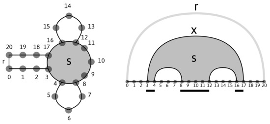
Figure 1. Left: a planar RNA secondary structure with a closing base pair $r=(0,20)$. Right: its diagram representation on the set of vertices $\left[19\right]$ with two additional vertices, 0 and 20, forming the rainbow $r=(0,20)$, the loop $s=[3,4]\cup [8,12]\cup [16,17]$ (shaded), and the corresponding intervals (underlined). The arc $x=(3,17)$ is the maximal arc of s, ${\alpha }_s=x$.

Secondary structures have been studied from the perspectives of enumerative combinatorics [9,10,11,12], algebraic combinatorics [13], matrix models [14,15], and topology [16,17,18].

In [10], a bijection between linear trees and secondary structures was presented. In [13], the authors enumerated k-non-crossing RNA structures by employing a bijection between k-non-crossing partial matchings and walks in the interior of the Weyl-chamber $C_0$ based on a certain bijection between oscillating tableaux and matchings [19,20,21]. The geometrical realization of a certain complex of secondary structures was studied in [22].

A key determinant of a sequence–structure pair is its thermodynamic stability, which is measured via its free energy. Given a sequence $\sigma$, RNA structure prediction algorithms identify structures by assuming minimal or low free energy with respect to $\sigma$ [23]. Given any RNA sequence–structure pair $(a,S)$, the free energy $\eta (a,S)$ is computed by adding all loop energy contributions [24,25], i.e., $\eta (a,S)={\sum }_{s\in S}\eta (a,s)$. Here, $\eta (a,s)$ depends on the loop type of s (hairpin, interior, multi-branch, etc.) and the particular nucleotides of the sequence a that appear in the loop s. Details on loop decompositions, partition functions, and recursive constructions for the folded structure—derived via polynomial-time dynamic programming (DP)—can be found in [9,23,26,27,28]. In [12], the notion of bi-secondary structures was introduced. Bi-secondary structures are central to identifying sequences that can realize two mutually exclusive minimum free energy (mfe) conformations. Such sequences naturally appear in the context of evolutionary transitions [29] and of RNA riboswitches, i.e., sequences that exhibit two distinct, stable configurations [30].

1.2. Motivation

This paper was motivated by the problem of computing thermodynamically stable sequences for two distinguished secondary structures, S and T [2]. The problem can be formalized as the computation of a sequence a that minimizes $\eta (a,S,T)$, where

$$\eta (a,S,T)=\sum _{s\in S}\eta (a,s)+\sum _{t\in T}\eta (a,t).$$

The sub-problems of the underlying DP routine are associated with sets of loops and recursively constructed by adding one loop at a time, where subsequently added nucleotides affect the energy calculation if they appear in multiple loops simultaneously; see Figure 2. This leads to the consideration of all such intersections as a simplicial complex, X, whose homology provides insights into the above optimization problem.

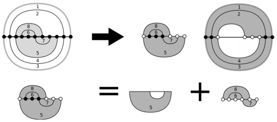
Figure 2. Top: a bi-structure decomposed into a distinguished sub-structure and its complement. The vertices contained in both (white) control the complexity of the dynamic programming (DP) routine in [2]. Bottom: the recursive step of the DP routine. Note that the recursion changes the set of white vertices by removing some and adding others.

In [1,31], we computed the simplicial homology groups of X and proved that only the second homology group carries information. This group was identified to be free, and its generators were identified as the crossing components within the diagram representation. All known RNA riboswitches exhibit one such crossing component, while random pairs of structures contain multiple crossing components.

The simplicial homology of X in [1] only allows us to express the existence of loop intersections. However, the crucial determinant for the algorithmic complexity of the DP routine in [2] is the size of such intersections; see Figure 2. The recursion is over the set of loops, successively examining one loop at a time. Each such examination affects certain vertices that the currently examined loop shares with the unprocessed loops.

It is thus natural to employ a homology theory that accounts for the intersection size. The notion of weighted homology as originally formulated [3], assigns a certain weight to each simplex, imposing specific divisibility conditions on these weights.

Our framework represents a variation on weighted homology as follows: We consider homology with coefficients in a discrete valuation ring, which, in fact, makes any divisibility constraints obsolete and allows us to deal with the cardinality of intersections in a natural way. The boundary operator introduced here is new, and so is our approach to connecting the weighted and simplicial homologies. More specifically, the construction of an inflation map relating $H_1(X^1)$ and $H_{1,R}(X^1)$ is a new technique. The computation of the weighted homology groups, $H_{0,R}$, $H_{1,R}(X)$, and $H_{2,R}(X)$, is also novel. Specifically, the idea of obtaining a combinatorial interpretation for the invariant factors in the structure theorems for $H_{0,R}$ and $H_{1,R}(X)$ via particular $X^1$-spanning trees is original. The chain maps between $C_n(X)$ and $C_{n,R}(X)$, which relate the $H_i(X)$ and $H_{i,R}(X)$ introduced here, are new and nontrivial. In particular, the injection $\mathrm{inj}:H_2(X)\to H_{2,R}(X)$ that induces the isomorphism $H_{2,R}(X)\cong R{\otimes }_{\mathbb{Z}}{H}_2(X)$ is a result of the fact that, in the expressions for the generators of $H_{2,R}(X)$, any triangle has a corresponding intersection size of one.

1.3. Organization

The paper is organized as follows: In Section 2, the simplicial loop complex of a bi-structure is introduced and the splicing of nucleotides is recalled [1]. In Section 3, the weighted complex of a bi-structure and a modified splicing procedure are discussed. In Section 4, the weighted homology and simplicial collapses [3,32] are introduced. In Section 5, a relative point of view is adopted by relating the simplicial and weighted homologies. Specifically, we introduce the inflation map, which maps classes of unweighted 1-cycles into corresponding weighted 1-cycles. In Section 6, we construct certain spanning trees that will be instrumental for proving our main results in Section 7. Here, we compute the weighted homology modules of bi-structures and provide combinatorial interpretations. The torsion module emerging in the zeroth homology stems from a recursive contraction scheme on the distinguished weighted spanning trees of the complex. The torsion of the first homology module can be understood via particular weighted edges that reference the aforementioned spanning tree. We conclude the paper with the computation of the second homology module, with all others being trivial. We integrate our results and outline future work in Section 8.

2. The Simplicial Loop Complex of a Bi-Structure

An RNA diagram S over the set $\left[n\right]:=\{1,\cdots ,n\}$ is a vertex-labeled graph—whose vertices represent nucleotides—drawn on the horizontal axis and labeled with elements of the set $\left[n\right]$. An arc $\alpha =(i,j),i<j$, is an ordered pair of vertices, which represents the base pairing between the i-th and j-th nucleotides. Each S-vertex can be paired with at most one other vertex, and the arc that connects them is drawn in the upper half-plane. An RNA diagram over the set $\left[n\right]$ is augmented with two additional vertices associated with positions 0 and $n+1$, together with the arc $(0,n+1)$, which is called the rainbow, representing the closing base pair of the external loop of the RNA structure; see [23]. The set of vertices $\{i,i+1,\dots ,j-1,j\}$ is called an interval, and is denoted by $[i,j]$. The set $[0,n+1]:=\{0,1,\cdots ,n,n+1\}$ is referred to as the backbone of the diagram. Two arcs, $(i,j)$ and $(p,q)$ with $i<p$, are called crossing if and only if $i<p<j<q$. S is called a secondary structure if it does not contain any crossing arcs. A loop s in a secondary structure S is represented as the disjoint union of intervals $s={\dot{\bigcup }}_{i=1}^k[a_i,b_i]$, such that $(a_1,b_k)$ and $(b_i,a_{i+1})$, for $1\le i\le k-1$, are arcs, and any other interval-vertices are unpaired. We denote by ${\alpha }_s$ the unique, maximal arc $(a_1,b_k)$ of the loop s, and we have a correspondence between loops and their maximal arcs; see Figure 1.

S-arcs and loops can be endowed with a partial order: $(k,l){\prec }_S(i,j)\iff i<k<l<j$. Abusing the notation, for the two loops $s_1,s_2\in S$, we write $s_1{\prec }_S{s}_2$ if ${\alpha }_{s_1}{\prec }_S{\alpha }_{s_2}$. Accordingly, (a) any unpaired vertex is contained in exactly one loop, (b) any non-rainbow arc appears in exactly two loops, and (c) the Hasse diagram of $(S,{\prec }_S)$ is a rooted tree $\mathrm{Tr}(S)$ with the rainbow arc as the root.

Given two secondary structures S and T, we refer to $R=(S,T)$ as a bi-secondary structure (bi-structure). Abusing the notation, we let $R=S\dot{\cup }T$ be the loop set of R. We represent a bi-structure $R=(S,T)$ with the S-arcs in the upper and the T-arcs in the lower half-plane along the same horizontal backbone.

Let $A=\{A_0,A_1,\dots ,A_m\}$ be a collection of finite sets. We call $B=\{A_{i_0},\dots ,A_{i_d}\}\subseteq A$ a d-simplex of A if ${\bigcap }_{k=0}^d{A}_{i_k}\ne ⌀$. We set $\Omega (B)={\bigcap }_{k=0}^d{A}_{i_k}$ and let $\omega (B)=|\Omega (B)|\ne 0$. Let $K_d(A)$ be the set of all d-simplices of A. Then, the complex (nerve) of A is $K(A)={\bigcup }_{d=0}^{\infty }{K}_d(A)\subseteq 2^A.$ A $d^{\prime }$-simplex $B^{\prime }\in K(A)$ is called a $d^{\prime }$-face of B if $d^{\prime }\le d$ and $B^{\prime }\subseteq B$. Let $B^{\prime }$ be a $d^{\prime }$-face of a maximal simplex B, where $d^{\prime }<d$. Then, $B^{\prime }$ is B-free if no other maximal simplex of $K(A)$ contains $B^{\prime }$ as a face. By construction, $K(A)$ is a simplicial complex. For a secondary structure S, $K(S)\cong \mathrm{Tr}(S)$ is a tree.

Let $R=(S,T)$ be a bi-structure with the loop complex $X={\dot{\bigcup }}_{d=0}^{\infty }{K}_d(R)$. Then, a simplicial order, ${\prec }_R$, is given by

$$r_1{\prec }_R{r}_2\iff \left\{\begin{array}{c}{r}_1,r_2\in T\mathrm{and}{r}_1{\prec }_T{r}_2\hfill \\ r_1,r_2\in S\mathrm{and}{r}_1{\prec }_S{r}_2\hfill \\ r_1\in S,r_2\in T\hfill \end{array}\right..$$

We specify a d-simplex, $\sigma \in X$, by the ordered $d+1$-tuple $\sigma =[r_{i_0},r_{i_1},...,r_{i_d}]$, where $r_{i_0}{\prec }_R{r}_{i_1}{\prec }_R\cdots {\prec }_R{r}_{i_d}$.

A 1-simplex $\tau =[r_{i_0},r_{i_1}]\in X$ is called pure if $r_{i_0}$ and $r_{i_1}$ are loops in the same secondary structure and mixed otherwise; see Figure 3.

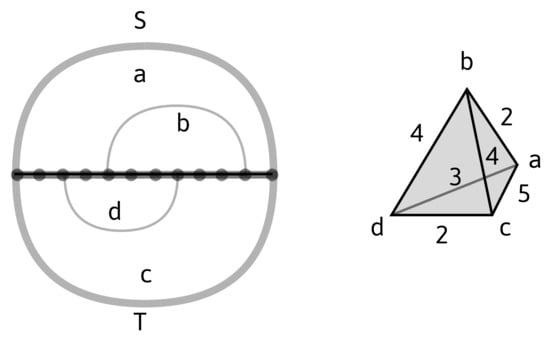
Figure 3. Left: a bi-structure $R=(S,T)$ with S-loops $a,b$, S-rainbow arc ${\alpha }_a$, T-loops $c,d$, and T-rainbow arc ${\alpha }_c$. Right: its weighted loop nerve $K_0(R)=\{a,b,c,d\},K_1(R)=\{[b,a],[b,c],[b,d],[d,c],[a,c],[a,d]\}$ (with $[b,a]$ and $[d,c]$ being pure edges, and any other edge being mixed), and $K_2(R)=\{[b,a,c],[b,d,c],[b,a,d],[a,d,c]\}$. We have $\omega (a)=7$, $\omega (b)=7$, $\omega (c)=8$, $\omega (d)=6$, $\omega ([b,a,c])=\omega ([b,d,c])=\omega ([b,a,d])=\omega ([a,d,c])=1$, while the weights of 1-simplices are displayed directly in the figure.

By construction, any 2-simplex $\Delta \in X$ contains exactly one pure and two mixed edges. Furthermore, X cannot contain simplices of a dimension greater than or equal to four, as that would imply that three or more loops in the same secondary structure intersect non-trivially. Moreover, for any $\sigma =[s_0,s_1,t_0,t_1]\in K_3(X)$, $1\le \omega (\sigma )\le 2$ and $\Omega (\sigma )\subset P=\{p\in [n]\mid \mathrm{deg}(p)=4\}$.

In [31], we investigated the effect of splicing a nucleotide p into two adjacent nucleotides $q_1,q_2$ such that the two arcs incident to p were resolved into two non-crossing arcs. In the case $\omega (\sigma )=2$, splitting does not change X, and if $\omega (\sigma )=1$, splitting induces a specific alteration: the removal of $\sigma$ from X, as well as a distinguished free edge, ${\tau }^{\sigma }$, and exactly two free triangles, ${\Delta }_1^{\sigma },{\Delta }_2^{\sigma }$, glued at ${\tau }^{\sigma }$. We refer to $({\tau }^{\sigma },{\Delta }_1^{\sigma },{\Delta }_2^{\sigma })$ as a $\sigma$-butterfly; see Figure 4.

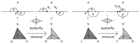
Figure 4. Splicing and removing tetrahedra together with their corresponding butterflies.

Lemma 1.

Let $R=(S,T)$ be a bi-structure with complex X; then, there exists a simple bi-structure $R=(S^{\prime },T^{\prime })$ with a complex $X^{\prime }<X$, where $X^{\prime }$ is derived from X by successively removing any 3-simplex, σ, together with an associated σ-butterfly.

Thus, successively splicing all nucleotides in P induces a bi-structure $(S^{\prime },T^{\prime })$, together with an associated complex $X^{\prime }<X$, which is obtained by removing all $\sigma$-butterflies and their corresponding $\sigma$s from X.

Removing a $\sigma$-butterfly and its corresponding $\sigma$ is equivalent to $X\searrow X^{\prime }$—a simplicial collapse consisting of two elementary collapses [32,33]. The first removes $\sigma$ and ${\Delta }_1^{\sigma }$, and the second removes ${\tau }^{\sigma }$ and ${\Delta }_2^{\sigma }$.

Proposition 1.

Let X be the loop complex of a bi-structure $R=(S,T)$, and let $X^{\prime }<X$ be an X-sub complex obtained by removing all 3-simplices, σ, from X, together with corresponding σ-butterflies. Then, $X^{\prime }$ is the complex of a bi-structure $R^{\prime }=(S^{\prime },T^{\prime })$ that satisfies ${(X^{\prime })}^2=X^{\prime }$ for any $k\ge 0$, $H_k(X^{\prime })\cong H_k(X)$.

Note that after splicing, we have simplified X to a complex of a bi-structure, $X^{\prime }$, thus reducing its maximum simplex dimension and maintaining its homology. In the following, we generalize this to weighted complexes.

3. $\mathbf{\mu }$-Splicings and the Weighted Complex of a Bi-Structure

We begin by modifying the splicing introduced in Section 2 as follows: Instead of replacing a nucleotide $p\in P$ by the two nucleotides $q_1<q_2$, we substitute it by three nucleotides, $q_1<a<q_2$, such that the arcs in R that share p as an endpoint now have endpoints $q_1$ and $q_2$, which are non-crossing, and a is unpaired. We call this a $\mu$-splicing of p.

Note that $\mu$-splicing and splicing all $p\in P$ have exactly the same effect on X—namely, eventually removing any 3-simplex $\sigma$ and a corresponding $\sigma$-butterfly. In terms of bi-structures, from $(S,T)$, $\mu$-splicing P produces the bi-structure $(S^{\prime },T^{\prime })$ augmented by a set of distinguished, unpaired nucleotides $A=\{a_1,\cdots ,a_n\}$, which only appear in 0- and 1-simplices. By construction, the complex $X^{\prime }$ of $(S^{\prime },T^{\prime })$ does not contain any 3-simplices. Furthermore, after $\mu$-splicing P, any distinguished nucleotide produced is flanked by two distinct endpoints of non-crossing arcs. Thus, for any simplex $\sigma \in X^{\prime }$, we have $h(\sigma )\ge 0$, where $h(\sigma )$ denotes the difference between the number of non-distinguished and distinguished nucleotides contained in $\sigma$. Note that h is a natural generalization of $\omega$ in the context of complexes of bi-structures. Accordingly, we define a weighted complex associated with a bi-structure as follows.

First, we recall that a ring R is called a discrete valuation ring if it is a Principal Ideal Domain (PID) with exactly one non-zero maximal ideal. Any irreducible element is a generator of this ideal and is called a uniformizer for R, and furthermore, any two such elements differ only up to multiplication with a unit.

Definition 1.

Let X be a complex of a bi-structure $(S,T)$ such that for any $\sigma \in X$, we have $h(\sigma )\ge 0$. Let $R\supset \mathbb{Z}$ be a discrete valuation ring with uniformizer π. We define the weight function $v:X\to R$, $v(\sigma )={\pi }^{h(\sigma )}$, and call $(X,v)$ the weighted complex of $(S,T)$.

Lemma 2.

Let $(S,T)$ be a bi-structure with no distinguished vertices and complex X. Let $(S^{\prime },T^{\prime })$ be derived from $(S,T)$ via μ-splicing P, and we denote its complex by $X^{\prime }$. Then, there exists an embedding

$$ϵ:(X^{\prime },v)⟶(X,v),$$

where $ϵ(X^{\prime })$ is a X-subcomplex obtained by removing any 3-simplices and associated butterflies. Moreover, ϵ is an embedding of weighted complexes: $\sigma =ϵ({\sigma }^{\prime })\Rightarrow v({\sigma }^{\prime })=v(\sigma )$.

Proof. 

Successively $\mu$-splicing P generates the series of complexes $X_{\left|P\right|}=X>\cdots >X_0=X^{\prime }$. By construction, given $X_i$ and a 3-simplex $\sigma$, the corresponding $\mu$-splicing at p replaces p with the triple $q_1^i<a_i<q_2^i$. Since $a_i$ is unpaired, $a_i$ is contained in exactly two loops, ${\lambda }_{i-1},{\mu }_{i-1}$, the only two loops that change size in terms of number of nucleotides when passing to $X_{i-1}$. Since the distinguished nucleotide contributes a $-1$, we note that $v({\lambda }_{i-1})=v({\lambda }_i)$ and $v({\mu }_{i-1})=v({\mu }_i)$; furthermore, $v([{\lambda }_i,{\mu }_i])=v([{\lambda }_{i-1},{\mu }_{i-1}])$. Any other $X_i$-simplex—differently from $\sigma$ and its $\sigma$-butterfly, which are removed—is not affected by the splicing, and consequently retains its weight in $X_{i-1}$, whence the lemma. □

4. Weighted Homology

Consider ${\partial }_n^v:C_{n,R}(X)\to C_{n-1,R}(X)$, where $C_{n,R}(X)$ denotes the free R-module generated by all n-simplices contained in X. Let ${\partial }_n^v$ be given by

$${\partial }_n^v(\sigma )=\sum _{i=0}^n\frac{v({\widehat{\sigma }}_i)}{v(\sigma )}·{(-1)}^i{\widehat{\sigma }}_i,$$

where the symbol $\frac{v({\widehat{\sigma }}_i)}{v(\sigma )}=\frac{{\pi }^{h({\widehat{\sigma }}_i)}}{{\pi }^{h(\sigma )}}$ is defined to be ${\pi }^{h({\widehat{\sigma }}_i)-h(\sigma )}$. This is, in view of $h(\sigma )\le h({\widehat{\sigma }}_i)$, a non-negative power of the uniformizer $\pi$ and, hence, still an element of the ring R. As a result, the boundary operator ${\partial }_n^v$ is well defined. Since $\frac{v({\widehat{\sigma }}_{i,j})}{v({\widehat{\sigma }}_i)}·\frac{v({\widehat{\sigma }}_i)}{v(\sigma )}=\frac{v({\widehat{\sigma }}_{j,i})}{v({\widehat{\sigma }}_j)}·\frac{v({\widehat{\sigma }}_j)}{v(\sigma )}$, we obtain ${\partial }_{n-1}^v({\partial }_n^v(\sigma ))=0$, i.e., ${\partial }_n^v$ is a boundary map.

Let $H_{n,R}(X)$ denote the ${\partial }_n^v$-homology groups. For $(Y,v)\le (X,v)$, we have

$$\begin{array}{ccccccc}0⟶& C_{n,R}(Y)& \stackrel{I}{⟶}& C_{n,R}(X)& \stackrel{J}{⟶}& C_{n,R}(X,Y)& ⟶0,\\ & \downarrow {\partial }^v& & \downarrow {\partial }^v& & \downarrow {\overline{\partial }}^v& \\ 0⟶& C_{n-1,R}(Y)& \stackrel{I}{⟶}& C_{n-1,R}(X)& \stackrel{J}{⟶}& C_{n-1,R}(X,Y)& ⟶0\end{array}$$

and we denote the relative homology groups by $H_{n,R}(X,Y)$. These are connected via the long exact sequence

$$\cdots ⟶H_{n,R}(X,Y)\stackrel{{\widehat{\partial }}_j^v}{⟶}{H}_{n-1}(Y)\stackrel{I_{*}}{⟶}{H}_{n-1}(X)\stackrel{J_{*}}{⟶}{H}_{n-1}(X,Y)\stackrel{{\widehat{\partial }}_{n-1}^v}{⟶}\cdots$$

Lemma 2 guarantees that, for any weighted complex $(X,v)$ of a bi-structure $(S,T)$, there exists a bi-structure $(S^{\prime },T^{\prime })$ with a weighted complex $(X^{\prime },v)$ such that $(X^{\prime },v)<(X,v)$ and where ${X^{\prime }}^2=X^{\prime }$. Thus, the relative homology groups $H_{k,R}(X,X^{\prime })$ and their associated long sequence are well defined.

However, a weighted complex does not have to be induced by a bi-structure. The previous definitions still hold as long as ${\sigma }^{\prime }\subseteq \sigma \Rightarrow v(\sigma )|v({\sigma }^{\prime })$ for an arbitrary $(X,v)$-pair. Weighted complexes represent a general combinatorial-algebraic framework that enhances the simplicial homology for a wide range of applications. The next proposition extracts the algebraic core of $\mu$-splicings; it represents a variation of [32], and it also appears in some form in [3].

Proposition 2.

Let $(X,v)$ be a weighted complex and let $\tau ,\sigma \in X$ such that: (a) τ is σ-free; (b) $v(\tau )=v(\sigma )$. Let Y be the X-subcomplex obtained by removing any $\tau \subset {\tau }^{\prime }\subset \sigma$ ($X\searrow Y$). Then,

$$\forall n\ge 0;H_{n,R}(X)\cong H_{n,R}(Y).$$

Proof. 

Claim 1. It suffices to prove the Lemma for a σ-free τ with the property $dim(\tau )+1=dim(\sigma )$.

We may assume that $\sigma =[v_0,\cdots ,v_k]$ and $\tau =\left[v_0\right]$. The lattice of sub-simplices of $\sigma$ is isomorphic to a binary k-cube, where cover relations are induced by face inclusions.

We prove by induction on k that a k-cube can be recursively decomposed into a sequence of pairs ${\mathsf{\Sigma }}_k={({\sigma }_i,{\tau }_i)}_{1\le i\le 2^{k-1}}$, where ${\sigma }_i$ is a maximal simplex with a free face ${\tau }_i$. The induction basis ${\mathsf{\Sigma }}_1=(\left[1\right],\left[0\right])$ is immediate.

For the induction step, note that a k-cube decomposes into two disjoint copies of a $(k-1)$-cube based on if the last coordinate is zero or one. By the induction hypothesis, for a $(k-1)$-cube, there exists a sequence, ${\mathsf{\Sigma }}_{k-1}={({\sigma }_i,{\tau }_i)}_{1\le i\le 2^{k-2}}$, with the desired properties; appending one or zero as the last coordinate yields two mappings from the $k-1$ cube into the k cube. By construction, these form a family of disjoint-type embeddings, i.e., their images are injective copies of the $k-1$-cube that are vertex disjoint in the k-cube. Accordingly, we obtain ${\mathsf{\Sigma }}_{k-1}^1={({\sigma }_i^1,{\tau }_i^1)}_i$ and ${\mathsf{\Sigma }}_{k-1}^0={({\sigma }_i^0,{\tau }_i^0)}_i$. As the two sub-cubes are disjoint, we can immediately construct the desired sequence for the k-cube, ${\mathsf{\Sigma }}_k={\mathsf{\Sigma }}_{k-1}^1{\mathsf{\Sigma }}_{k-1}^0$; the claim follows.

Claim 2. Let $X\searrow Y$, where $\sigma \in X$ maximal, τ is σ-free, and $dim(\tau )+1=dim(\sigma )=k$. Then, for any $n\ge 0$, $H_{n,R}(X,Y)=0$.

Note that only $C_{k,R}(X,Y)$ and $C_{k-1,R}(X,Y)$ are non-trivial. $C_{k+1,R}(X,Y)=0$ implies $\mathrm{Im}({\widehat{\partial }}_{k+1}^v)=0$; hence, $H_{k,R}(X,Y)=\mathrm{Ker}({\widehat{\partial }}_k^v)$. Note that $C_{k,R}(X,Y)={⟨\sigma ⟩}_R$, so ${\widehat{\partial }}_k^v(r·\sigma )=0$ implies $r=0$; thus, $H_{k,R}(X,Y)=0$. Similarly, $C_{k-1,R}(X,Y)={⟨\tau ⟩}_R$, so $\mathrm{Ker}({\widehat{\partial }}_{k-1}^v)\subset C_{k-1,R}(X,X^{\prime })$ is also generated by $\tau$. Now, ${\widehat{\partial }}_k^v(\sigma )=v(\tau )/v(\sigma )·\tau =\tau$, and so $H_{k-1,R}(X,Y)=0$. Finally, for $n\ne k,k-1$, $\mathrm{Ker}({\widehat{\partial }}_n^v)\subset C_{n,R}(X,Y)=0$, so $H_{n,R}(X,Y)=0$ for any $n\ne k,k-1$, and Claim 2 follows.

The proposition is implied in view of Claim 2 and the following long exact sequence:

$$⟶H_{n+1,R}(X,Y)\stackrel{{\partial }_n^v}{⟶}{H}_{n,R}(Y)\stackrel{I_{*}}{⟶}{H}_{n,R}(X)\stackrel{J_{*}}{⟶}{H}_{n,R}(X,Y)⟶.$$

 □

In view of $X\searrow X^{\prime }$ and $v({\tau }^{\sigma })=v({\Delta }_1^{\sigma })=v({\Delta }_2^{\sigma })=v(\sigma )$, for any $\sigma \in X^3$ and its corresponding $\sigma$-butterfly, Proposition 2 implies the following.

Corollary 1.

Let $(X,v)$ be the complex of the bi-structure $(S,T)$, and let $(X^{\prime },v)$ be the complex of $(S^{\prime },T^{\prime })$ that is obtained by completely μ-splicing $(S,T)$. Then,

$$\forall k\ge 0,H_{k,R}(X^{\prime })\cong H_{k,R}(X).$$

5. The Inflation Map

In view of Corollary 1, we can assume that X is the complex of a bi-structure with the property $X^2=X$, where $X^k$ denotes the simplicial complex induced by all k-simplices in X [34]. Clearly, the natural embedding $X^1\to X$ is an embedding of weighted complexes, and we have the exact sequence

$$\begin{array}{ccccccc}0⟶& C_{n,R}(X^1)& \stackrel{I}{⟶}& C_{n,R}(X)& \stackrel{J}{⟶}& C_{n,R}(X,X^1)& ⟶0,\\ & \downarrow {\partial }^v& & \downarrow {\partial }^v& & \stackrel{{\overline{\partial }}^v}{\downarrow }& \\ 0⟶& C_{n-1,R}(X^1)& \stackrel{I}{⟶}& C_{n-1,R}(X)& \stackrel{J}{⟶}& C_{n-1,R}(X,X^1)& ⟶0\end{array}$$

producing the long exact sequence

$$0\stackrel{I_{*}}{⟶}{H}_{2,R}(X)\stackrel{J_{*}}{⟶}{H}_{2,R}(X,X^1)\stackrel{{\widehat{\partial }}_2^v}{⟶}{H}_{1,R}(X^1)\stackrel{I_{*}}{⟶}{H}_{1,R}(X)⟶0.$$

(1)

We now adopt a relative point of view by relating the simplicial homology $H_k(X)$ to the weighted homology $H_{k,R}(X)$. To this end, we consider the following two segments of the long homology sequences

$$\begin{array}{ccccccccc}0⟶& H_{2,R}(X)& \stackrel{J_{*}}{⟶}& H_{2,R}(X,X^1)& \stackrel{{\widehat{\partial }}_2^v}{⟶}& H_{1,R}(X^1)& \stackrel{I_{*}}{⟶}& H_{1,R}(X)& ⟶0,\\ & \mathrm{inj}\uparrow & & & \mathrm{inj}\uparrow & & ?\uparrow & & & \\ 0⟶& H_2(X)& \stackrel{J_{*}}{⟶}& H_2(X,X^1)& \stackrel{{\widehat{\partial }}_2}{⟶}& H_1(X^1)& \stackrel{I_{*}}{⟶}& ⟶0& \end{array}$$

where the surjectivity of ${\widehat{\partial }}_2$ is given by $H_1(X)=0$ [1].

While these sequences belong to different categories, the first two vertical maps are natural injections and relate simplicial and weighted homology modules.

Indeed, the first vertical injection is induced by chain maps of the form ${\theta }_n:C_n(X)\stackrel{}{\to }{C}_{n,R}(X)$, $\theta ({\sum }_i{n}_i{\sigma }_i)={\sum }_i{n}_{i}v({\sigma }_i){\sigma }_i$, which make the following diagram commutative:

$$\begin{array}{ccccc}\hfill \cdots ⟶& C_n(X)& \stackrel{{\partial }_n}{⟶}& C_{n-1}(X)& ⟶\cdots \\ & \downarrow {\theta }_n& & \downarrow {\theta }_{n-1}& \\ \cdots ⟶\hfill & C_{n-1}(X)& \stackrel{{\partial }_n^v}{⟶}& C_{n-1,R}(X)& ⟶\cdots \end{array}$$

The second vertical injection is given by the fact that, since $\mathbb{Z}\subset R$, $C_2(X)$ is an R-submodule of $C_{2,R}(X)$ and, by construction, $H_2(X,X^1)=C_2(X)$ and $H_{2,R}(X,X^1)=C_{2,R}(X)$.

This motivates us to ask if there exists a $\mathbb{Z}$-linear map that makes the above diagram commutative. It turns out that such a map exists and will prove useful for understanding $H_{1,R}(X)$.

Lemma 3.

The mapping

$$\mathrm{infl}:H_1(X^1)\to H_{1,R}(X^1),\mathrm{infl}(c)={\widehat{\partial }}_2^v\left(\sum _i{\Delta }_i\right),$$

where $c=\widehat{{\partial }_2}({\sum }_i{\Delta }_i)$, is well defined and $\mathbb{Z}$-linear; the following diagram is commutative:

$$\begin{array}{ccc}{H}_{2,R}(X,X^1)& \stackrel{{\widehat{\partial }}_2^v}{⟶}& H_{1,R}(X^1)\\ \mathrm{inj}\uparrow & & \mathrm{infl}\uparrow \\ H_2(X,X^1)& \stackrel{{\widehat{\partial }}_2}{⟶}& H_1(X^1).\end{array}$$

Proof. 

By construction, it suffices to show that infl is well defined. Observe that, in view of sequence (1), ${\widehat{\partial }}_2$ is surjective. Hence, any $c\in H_1(X^1)$ can be expressed as $c={\sum }_i{\widehat{\partial }}_2({\Delta }_i)$, where ${\sum }_i{\Delta }_i$ is unique, modulo elements of $\mathrm{Ker}({\widehat{\partial }}_2)$. Secondly, in [31], we showed that

$$\mathrm{Ker}({\widehat{\partial }}_2)=\underset{\beta }{⨁}\mathbb{Z}{\nabla }_{\beta },$$

where ${\nabla }_{\beta }={\sum }_j{\Delta }_j$; ${\Delta }_j$ is contained in the $(S,T)$-crossing component $\beta$ and $v({\Delta }_j)=1$.

Any face e contained in ${\widehat{\partial }}_2({\nabla }_{\beta })$ appears with opposite signs in two distinct the 2-simplices ${\Delta }_e$ and ${\Delta }_e^{\prime }$, where $v({\Delta }_e)=v({\Delta }_e^{\prime })=1$. Therefore,

$${\widehat{\partial }}_2^v({\nabla }_{\beta })=\sum _{e\in {\widehat{\partial }}_2({\nabla }_{\beta })}\left(\frac{v(e)}{v({\Delta }_e)}·e-\frac{v(e)}{v({\Delta }_e^{\prime })}·e\right)=0,$$

i.e., $\mathrm{inj}({\nabla }_{\beta })\in \mathrm{Ker}({\widehat{\partial }}_2^v)$; infl is well defined, and a lemma follows. □

We next employ $\mathrm{infl}:H_1(X^1)\to H_{1,R}(X^1)$ to obtain information about $H_{1,R}(X^1)$. $X^1$ is connected, and for a spanning tree ${\mathcal{T}}_{X^1}$, the free generators of $H_1(X^1)$ are in bijection with $\kappa$’s mixed $X^1$ cycle closing edges for ${\mathcal{T}}_{X^1}$. A generator $c_{\kappa }\in H_1(X^1)$ is a sum of edges $u_j\in {\mathcal{T}}_{X^1}$ and the closing edge $\kappa$, with each such edge appearing exactly once. We fix ${\mathcal{T}}_{X^1}$ as follows: Consider the trees ${\mathcal{T}}_S,{\mathcal{T}}_T$ of the sub-complexes for S and T, respectively, and let ${\mathcal{T}}_{X^1}$ be the tree obtained by connecting the ${\mathcal{T}}_S,{\mathcal{T}}_T$-roots with the mixed edge $\omega$, corresponding to the two rainbow loops.

Lemma 4.

The following sequence of R modules is exact:

$$0⟶R{\otimes }_{\mathbb{Z}}\mathrm{infl}{(H_1(X^1))}^{\stackrel{\mathrm{inj}}{⟶}}{H}_{1,R}(X^1)\stackrel{I_{*}}{⟶}{H}_{1,R}(X)⟶0.$$

Proof. 

With ${\mathcal{T}}_{X^1}$ as above, consider a generator $c_{\kappa }={\sum }_j{u}_j\in H_1(X^1)$ where, for $1<j<n$, $u_j$ are pure S- or T-edges and $u_1=\omega$ while $u_n=\kappa$. Since ${\widehat{\partial }}_2$ is surjective, we can also write

$$c_{\kappa }=\sum _i{\widehat{\partial }}_2({\Delta }_i)=\sum _i(e_{0,i}-e_{1,i}+e_{2,i}).$$

This involves additional mutually canceling edges, k, all of which are mixed and appear as faces of pairs of 2-simplices, $({\Delta }_k,{\Delta }_k^{\prime })$. Without loss of generality (w.l.o.g.), we can traverse the cycle $c_{\kappa }$ beginning at $\omega$ via the pure S-edges until we arrive at $\kappa$, after which we return back to $\omega$ via the pure T-edges. Any $({\Delta }_k,{\Delta }_k^{\prime })$ pair satisfies either $v({\Delta }_k)=v({\Delta }_k^{\prime })$ or $v({\Delta }_k)\ne v({\Delta }_k^{\prime })$, and we accordingly categorize the k edges into $k_{\alpha }$- and $k_{\beta }$-edges, respectively. As a result, in

$$\mathrm{infl}(c_{\kappa })=\sum _i{\widehat{\partial }}_2^v({\Delta }_i)=\sum _i\left(\frac{v(e_{0,i})}{v({\Delta }_i)}·e_{0,i}-\frac{v(e_{1,i})}{v({\Delta }_i)}·e_{1,i}+\frac{v(e_{2,i})}{v({\Delta }_i)}·e_{2,i}\right),$$

$k_{\beta }$-edges persist with the coefficient, say $f(k_{\beta })\in R$, while all $k_{\alpha }$-edges cancel. Hence,

$$\mathrm{infl}(c_{\kappa })=\sum _j\frac{v(u_j)}{v({\Delta }_j)}·u_j+\sum _{k_{\beta }}f(k_{\beta })·k_{\beta },$$

where $u_j\in {\widehat{\partial }}_2({\Delta }_j)$. Note that only $\kappa$ and $\omega$ are mixed $c_{\kappa }$-edges, and so $\left\{u_j\right\}\cap \left\{k_{\beta }\right\}=⌀$.

Any set M of $c_{\kappa }$-cycles induces a set of distinct mixed faces $\omega ,{\kappa }_1,\cdots ,{\kappa }_h$. In the two sub-trees of S and T formed by the respective pure edges of the $c_{\kappa }$-paths, these mixed faces connect an S-leaf with a T-minimal vertex or a T-leaf with an S-minimal vertex. By construction, these edges are distinct from any of the $k_{\beta }$ produced by any M-cycle, and the coefficients of any of these $c_{{\kappa }_i}$$1\le i\le h$ in a linear combination ${\sum }_{c_{\kappa }\in M}{r}_{\kappa }·\mathrm{infl}(c_{\kappa })=0$ are zero. Iterating this argument, we arrive at

$$\sum _{\kappa }{r}_{\kappa }·\mathrm{infl}(c_{\kappa })=0\Rightarrow r_{\kappa }=0.$$

Accordingly, $\{\mathrm{infl}(c_{\kappa })\mid \kappa \}$ freely generate ${⟨\{\mathrm{infl}(c_{\kappa })\mid \kappa \}⟩}_R$, and the following diagram is commutative:

$$\begin{array}{cccccc}{H}_{2,R}(X,X^1)& \stackrel{{\widehat{\partial }}_2^v}{⟶}& H_{1,R}(X^1)& \stackrel{I_{*}}{⟶}& H_{1,R}(X)& ⟶0\\ \mathrm{inj}\uparrow & & \mathrm{infl}\uparrow & & & \\ H_2(X,X^1)& \stackrel{{\widehat{\partial }}_2}{⟶}& H_1(X^1)& \stackrel{I_{*}}{⟶}& 0\\ & & \uparrow & & & \\ & & 0& & & \end{array}$$

Since $\mathrm{Im}({\widehat{\partial }}_2^v)=R{\otimes }_{\mathbb{Z}}\mathrm{Im}(\mathrm{infl})$, we have $H_{1,R}(X)\cong H_{1,R}(X^1)/(R{\otimes }_{\mathbb{Z}}\mathrm{Im}(\mathrm{infl})),$ whence

$$0⟶R{\otimes }_{\mathbb{Z}}\mathrm{infl}(H_1(X^1))\stackrel{\mathrm{inj}}{⟶}{H}_{1,R}(X^1)\stackrel{I_{*}}{⟶}{H}_{1,R}(X)⟶0.$$

 □

6. The Rank of ${\mathit{H}}_{\mathbf{1}\mathbf{,}\mathit{R}}\mathbf{\left(}{\mathit{X}}^{\mathbf{1}}\mathbf{\right)}$

Next, we compute the rank of $H_{1,R}(X^1)$ by constructing a basis. Note that an element in $H_1(X^1)$ is a sum of cycles, and it is natural to ask what the analogue of a cycle in $H_{1,R}(X^1)$ is.

Let $c^{\prime }={\sum }_i{e}_i\in H_1(X^1)$ be minimal in terms of the number of edges it contains. A straightforward computation shows that there exist $r_i\in R$ with ${\partial }_1^v({\sum }_i{r}_i·e_i)=0$, where the multi-set ${(r_i)}_i$ is unique up to a scalar factor. This shows that, except for a scalar multiple, minimal $H_1(X^1)$ cycles determine the distinguished $H_{1,R}(X^1)$ cycles, and we shall call a cycle $c={\sum }_i{r}_i{e}_i\in H_{1,R}(X^1)$ elementary if $gcd(\left\{r_i\right\})=1$ and ${\sum }_i{e}_i\in H_1(X^1)$ is a minimal cycle. An elementary cycle is precisely the $H_{1,R}(X^1)$-analogue of a minimal $H_1(X^1)$-cycle.

In view of $X^1$ being connected, a basis of $H_1(X^1)$ can be comprised of all minimal cycles derived from a fixed $X^1$-spanning tree $\mathcal{T}$: Any $X^1$ non-tree edge added to this tree results in a unique minimal cycle in the basis that is labeled by the edge. One key observation here is that $\left\{{\partial }_1(e)\right|e\in \mathcal{T}\}$ generates ${\partial }_1(C_1(X^1))$ for an arbitrary spanning tree $\mathcal{T}$ of $X^1$.

To derive a basis of $H_{1,R}(X^1)$ in an analogous fashion, an arbitrary choice of an $X^1$-spanning tree is no longer sufficient because of the weights involved. However, in the following, we construct a distinguished tree ${\mathcal{T}}_{X^1}^{\#}$ that is particularly well suited to the understanding of the embedding of $H_1(X^1)$ into $H_{1,R}(X^1)$.

Lemma 5.

There exists an $X^1$-spanning tree, ${\mathcal{T}}_{X^1}^{\#}$, such that the following sequence is exact:

$$0⟶C_{1,R}({\mathcal{T}}_{X^1}^{\#})\stackrel{{\partial }_1^v}{⟶}{C}_{0,R}(X)\stackrel{\mathrm{proj}}{⟶}{H}_{0,R}(X)⟶0.$$

Proof. 

It suffices to construct ${\mathcal{T}}_{X^1}^{\#}$ such that ${\partial }_1^v({⟨{\mathcal{T}}_{X^1}^{\#}⟩}_R)$$={\partial }_1^v({⟨X^1⟩}_R)$. To this end, we fix an arbitrary $X^1$-spanning tree ${\mathcal{T}}_0$ and let $M=X^1\setminus {\mathcal{T}}_0$. We examine M-edges one by one, yielding a chain of processed edges, $⌀=M_0\subset ,\cdots ,\subset M_{k-1}\subset M_k$, and a sequence of trees, ${\mathcal{T}}_0,\cdots ,{\mathcal{T}}_{k-1},{\mathcal{T}}_k$. We claim that these have the property ${\partial }_1^v({⟨{\mathcal{T}}_k⟩}_R)={\partial }_1^v({⟨M_k\cup {\mathcal{T}}_0⟩}_R)$.

The above holds trivially for $k=0$, and we assume that $M_{k-1}$ and ${\mathcal{T}}_{k-1}$ are constructed with ${\partial }_1^v({⟨{\mathcal{T}}_{k-1}⟩}_R)={\partial }_1^v({⟨M_{k-1}\cup {\mathcal{T}}_0⟩}_R)$. Let $e_k\in M\setminus M_{k-1}$ and set $M_k=M_{k-1}\bigcup \left\{e_k\right\}$. Then, there exist $r_e\in R$ such that ${\sum }_{e\in \left\{e_k\right\}\cup {\mathcal{T}}_{k-1}}{r}_e{\partial }_1^v(e)=0$. Letting $r=gcd\left\{r_e\right\}$ and $r_e=r{r}_e^{\prime }$ leads to ${\sum }_{e\in \left\{e_k\right\}\cup {\mathcal{T}}_{k-1}}{r}_e^{\prime }{\partial }_1^v(e)=0,$ where, by construction, at least one edge has a coefficient of one. In case the $r_{e_k}^{\prime }=1$, set ${\mathcal{T}}_k={\mathcal{T}}_{k-1}$. Otherwise, remove a ${\mathcal{T}}_{k-1}$-edge with coefficient one, and add $e_k$ to ${\mathcal{T}}_{k-1}$, obtaining ${\mathcal{T}}_k$. Note then that

$${\partial }_1^v({⟨{\mathcal{T}}_k⟩}_R)={\partial }_1^v({⟨\left\{e_k\right\}\cup {\mathcal{T}}_{k-1}⟩}_R)={\partial }_1^v({⟨\left\{e_k\right\}⟩}_R)+{\partial }_1^v({⟨M_{k-1}\cup {\mathcal{T}}_0⟩}_R)={\partial }_1^v({⟨M_k\cup {\mathcal{T}}_0⟩}_R).$$

By induction, when the processes terminates, it yields the desired ${\mathcal{T}}_{X^1}^{\#}$. □

${\mathcal{T}}_{X^1}^{\#}$ induces a new set of closing edges ${\kappa }^{\#}$ and the associated minimal $H_1(X^1)$-cycles $c_{{\kappa }^{\#}}$. We shall show that the corresponding elementary cycles constitute a basis of $H_{1,R}(X^1)$.

Proposition 3.

There exists an isomorphism

$$H_{1,R}(X^1)\cong R{\otimes }_{\mathbb{Z}}{H}_1(X^1).$$

Furthermore, $H_{1,R}(X^1)$ is freely generated by the set of elementary cycles $c_{{\kappa }^{\#}}$ and has rank $e-v+1$, where e and v are the numbers of 1- and 0-simplices in $X^1$.

Proof. 

$H_{1,R}(X^1)$ is free, as it is a sub-module of the finitely generated free module over the PID R and $C_{1,R}(X^1)$. By construction, to each $c_{{\kappa }^{\#}}\in H_1(X^1)$, there corresponds a unique elementary $H_{1,R}(X^1)$-cycle $c_{{\kappa }^{\#}}^v$, whose ${\kappa }^{\#}$ coefficient is one. Furthermore, $c_{{\kappa }^{\#}}^v$ is non-torsion in $H_{1,R}(X^1)$; if $r·c_{{\kappa }^{\#}}^v=0$, R being an integral domain implies $r=0$.

Claim. Any $c\in H_{1,R}(X^1)$ has the representation $c={\sum }_{\kappa }{r}_{{\kappa }^{\#}}{c}_{{\kappa }^{\#}}^v$ with a unique $r_{{\kappa }^{\#}}\in R$.

We proceed by induction on the number of ${\mathcal{T}}_{X_1}^{\#}$-closing edges in c.

To establish the induction basis, let $r_{{\kappa }^{\#}}{\kappa }^{\#}$ be the unique term that contains ${\kappa }^{\#}$ in c. Using the fact that ${\kappa }^{\#}$ appears with a coefficient of one in $c_{{\kappa }^{\#}}^v$, we derive $c=r_{{\kappa }^{\#}}{c}_{{\kappa }^{\#}}^v$.

For the induction step, distinguishing $r_{{\kappa }_1^{\#}}{\kappa }_1^{\#}$ as a closing edge summand in c, we have $c-r_{{\kappa }_1^{\#}}·c_{{\kappa }_1^{\#}}^v=\tilde{c}\in H_{1,R}(X^1)$ with ${\kappa }_1^{\#}\notin \tilde{c}$. By inductive hypothesis, $\tilde{c}={\sum }_{{\kappa }^{\#}\in \tilde{c}}{r}_{{\kappa }^{\#}}·c_{{\kappa }^{\#}}^v$ with unique coefficients $r_{{\kappa }^{\#}}$, hence the claim.

From the claim and the fact that the $c_{{\kappa }^{\#}}^v$ are non-torsion, we conclude that

$$H_{1,R}(X^1)\cong \underset{\kappa }{⨁}R{c}_{{\kappa }^{\#}}^v\cong R{\otimes }_{\mathbb{Z}}{H}_1(X^1),$$

hence the proposition. □

7. The Modules of the Weighted Homology

By Lemma 5, we have

$$\mathrm{rnk}(\mathrm{Im}({\partial }_1^v))=\mathrm{rnk}({\partial }_1^v({⟨{\mathcal{T}}_{X^1}^{\#}⟩}_R))=v-1,$$

from which $\mathrm{rnk}(C_{0,R}(X)/\mathrm{Im}({\partial }_1^v))=1$.

Since $C_{0,R}(X)/\mathrm{Im}({\partial }_1^v)$ is a module over the PID R, we arrive at

$$H_{0,R}(X)\cong C_{0,R}(X)/\mathrm{Im}({\partial }_1^v)\cong M_{\pi }\oplus R,$$

where $n_1\ge \cdots n_{v-1}\ge 0$, and $M_{\pi }={⨁}_{j=1}^{v-1}R/({\pi }^{n_j})$ is the $\pi$-torsion module of $H_{0,R}(X)$.

We shall proceed by computing $M_{\pi }$. Note that the ${\mathcal{T}}_{X^1}^{\#}$-tree is a spanning tree of $X^1$, and $\left\{{\partial }_1^v(e)\right|e\in {\mathcal{T}}_{X^1}^{\#}\}$ generates $\mathrm{Im}({\partial }_1^v)$. Thus, we can compute $H_{0,R}(X)$ via ${\mathcal{T}}_{X^1}^{\#}$. To this end, we process ${\mathcal{T}}_{X^1}^{\#}$ as follows: We select a ${\mathcal{T}}_{X^1}^{\#}$-vertex $u_i$ and an incident edge $e_i=(u_j,u_i)$ for which ${log}_{\pi }\frac{v(u_i)}{v(e_i)}$ is minimal. We contract $e_i$ onto $u_j$ by removing $u_i$ and replacing any edges of the form $(u_k,u_i)$ with $(u_k,u_j)$ while maintaining their original weights $v(u_k,u_j):=v(u_k,u_i)$. Recursively contracting all $(v-1)$ edges in ${\mathcal{T}}_{X^1}^{\#}$ produces a sequence of trees ${\mathcal{T}}_{X^1}^{\#}=T_0,\cdots ,T_{v-1}$, where $T_{v-1}=u_v$ is a single vertex at which point the process terminates. Relabeling the ${\mathcal{T}}_{X^1}^{\#}$-vertices, we may assume that $u_i$ is removed at the ith step of this process.

Theorem 1.

There exists an isomorphism

$$H_{0,R}(X)\cong \left(\underset{i=1}{\overset{v-1}{⨁}}R/({\pi }^{n_i})\right)\oplus R,$$

where $n_i={log}_{\pi }\frac{v(u_i)}{v(e_i)}$, as described above.

Proof. 

Let $E_m=\{e_i=(u_{a_i},u_i)\mid 0\le i\le m\}$ denote the set of recursively contracted edges up to and including the mth step. Set $e_i=(u_i,u_{a_i})$, $x_i=u_i-\frac{v(u_{a_i})}{v(u_i)}{u}_{a_i}$, and $x_v=u_v$, where the formal fractions are well defined by the minimality of the denominator exponent. Note then that ${\partial }_1^v(e_i)=\frac{v(u_i)}{v(e_i)}{u}_i-\frac{v(u_{a_i})}{v(e_i)}{u}_{a_i}=\frac{v(u_i)}{v(e_i)}{x}_i:=w_i{x}_i$.

Claim 1. ${\partial }_1^v({⟨E_i\cup T_i⟩}_R)=\mathrm{Im}({\partial }_1^v)$ for any $0\le i\le v-1$.

We proceed by induction on i, where Lemma 5 implies the induction basis $i=0$. Consider the contraction at step i: $E_i=E_{i-1}\cup \{e_i=(u_{a_i},u_i)\}$. A $T_{i-1}$-edge of the form $f_k=(u_k,u_i)$ induces the $T_i$-edge $f_k^{\prime }=(u_k,u_{a_i})$ with $v(f_k)=v(f_k^{\prime })$. Then,

$${\partial }_1^v(f_k^{\prime })-{\partial }_1^v(f_k)=\frac{v(u_k)}{v(f_k^{\prime })}{u}_k-\frac{v(u_{a_i})}{v(f_k^{\prime })}{u}_{a_i}-\left[\frac{v(u_k)}{v(f_k)}{u}_k-\frac{v(u_i)}{v(f_k)}{u}_i\right]={\partial }_1^v(e_i)$$

implies ${\partial }_1^v({⟨E_{i-1}\cup T_{i-1}⟩}_R)={\partial }_1^v({⟨E_i\cup T_i⟩}_R)$, and Claim 1 follows by induction.

Claim 2. $C_{0,R}(X)={⨁}_{i=1}^{v}R{x}_i$.

Let $z={\sum }_{j=1}^v{r}_j^{\prime }{u}_j\in C_{0,R}(X)$, where $u_i$ is removed from $T_{i-1}$ at the ith contraction step. We rewrite the z in terms of the $x_i$. This is done recursively, starting with $u_1$, as follows: Let $C_p(u_q)$ be the coefficient of $u_q$ at step p. Then, $x_i=u_i-\frac{v(u_{a_i})}{v(u_i)}{u}_{a_i}$ implies $C_i(u_i)u_i=C_i(u_i)x_i+C_i(u_i)\frac{v(u_{a_i})}{v(u_i)}{u}_{a_i}$, and we obtain the updated $u_{a_i}$-coefficient

$$C_{i+1}(u_{a_i})=C_i(u_{a_i})+C_i(u_i)\frac{v(u_{a_i})}{v(u_i)}.$$

Processing all $u_i$, we arrive at $z={\sum }_{=1}^{v-1}{r}_i{x}_i+r_v{x}_v$, and Claim 2 follows.

Claim 3. $H_{0,R}(X)\cong \left({⨁}_{i=1}^{v-1}R{\overline{x}}_i\right)\oplus R{x}_v$ with ${\overline{x}}_i=x_i+{⟨{\partial }_1^v(e_i)⟩}_R$.

By Claim 2, we have $H_{0,R}(X)=({⨁}_{i=1}^{v}R{x}_i)/\mathrm{Im}({\partial }_1^v)$, and we make the following ansatz:

$$\phi :H_{0,R}(X)⟶\left(\underset{i=1}{\overset{v}{⨁}}R{\overline{x}}_i\right)\oplus R{x}_v,\phi \left((\sum _{i=1}^{v-1}{r}_i{x}_i+r_v{x}_v)+\mathrm{Im}({\partial }_1^v)\right)=\sum _{i=1}^{v-1}{r}_i{\overline{x}}_i+r_v{x}_v.$$

First, $\phi$ is a well-defined homomorphism: Suppose ${\sum }_i{r}_i{x}_i-{\sum }_i{r}_i^{\prime }{x}_i\in \mathrm{Im}({\partial }_1^v)$. Since $x_v$ is linearly independent from $x_i$, $1\le i\le v-1$, this immediately implies that $r_v=r_v^{\prime }$. Claim 1 guarantees that $\mathrm{Im}({\partial }_1^v)={\partial }_1^v({⟨E_{v-1}⟩}_R)$, and consequently, there exist unique coefficients, ${\alpha }_i$, such that

$$\sum _{i=1}^{v-1}{r}_i{x}_i-\sum _{i=1}^{v-1}{r}_i^{\prime }{x}_i={\partial }_1^v(\sum _{i=1}^{v-1}{\alpha }_i{e}_i).$$

In view of ${\partial }_1^v(e_i)=n_i{x}_i$, we obtain

$$\sum _{i=1}^{v-1}{r}_i{x}_i-\sum _{i=1}^{v-1}{r}_i^{\prime }{x}_i=\sum _{i=1}^{v-1}{\alpha }_i{\partial }_1^v(e_i)=\sum _{i=1}^{v-1}{s}_i{n}_i{x}_i.$$

The linear independence of $x_i$, in turn, implies that $(r_i-r_i^{\prime })=s_i{n}_i$ for any i, from which $(r_i-r_i^{\prime })x_i=s_i{\partial }_1^v(e_i)$, and thus, $r_i{\overline{x}}_i=r_i^{\prime }{\overline{x}}_i$.

$\phi$ is, by construction, surjective and does not have a nontrivial kernel from which Claim 3 follows.

By construction, $R{x}_v\cong R$, and as for the direct summands $R{\overline{x}}_k$, for $1\le k\le v-1$, we consider the mapping $h:R{\overline{x}}_k\to R/R{n}_k$, $h(r{\overline{x}}_k)=rmod{n}_k$. Suppose that $(r_k-r_k^{\prime })x_k=s_k{\partial }_1^v(e_k)$; then, ${\partial }_1^v(e_k)=n_k{x}_k$ implies that $(r_k-r_k^{\prime })=s_k{n}_k$, so h is well defined. Clearly h is surjective, and it remains to check the injectivity. $h(r{\overline{x}}_k)=0$ implies that $r=s{n}_k$ and $s{n}_k{x}_k=s{\partial }_1^v(e_k)$ implies that $r{\overline{x}}_k=\overline{0}$, hence the theorem. □

We proceed by analyzing $H_{1,R}(X)$. We begin with the expression for $\mathrm{infl}(c_{{\kappa }^{\#}})$ in Lemma 4:

$$\mathrm{infl}(c_{{\kappa }^{\#}})=\sum _j\frac{v(u_j)}{v({\Delta }_j)}·u_j+\sum _{k_{\beta }}f(k_{\beta })·k_{\beta },$$

where ${\Delta }_j$ is the 2-simplex containing the edge $u_j$, and $k_{\beta }$ are mixed edges that appear when transitioning between 2-simplices with different weights that share a $k_{\beta }$ face.

The “troublemakers” here are the off-diagonal terms of the embedding, $k_{\beta }$, which stem from passing from trivial to nontrivial crossing components and vice versa. We shall eliminate such transitions by appropriately deforming X without affecting its homology. We then have to check that the deformation gives rise to an inflation map that is just a restriction of the original inflation map for X. Let $\Delta \in X$ be a 2-simplex corresponding to a non-crossing arc, i.e., $\Delta$ is maximal in X. W.l.o.g., we can assume that $\Delta =[s_1,s_2,t]$ with $s_1,s_2\in S,t\in T$. Then, $\tau =[s_1,s_2]$ is $\Delta$-free, and by construction, $v(\tau )=v(\Delta )=2$. Removing $\tau$ and $\Delta$ from X produces a sub-complex $X^{\prime }$ with $X\searrow X^{\prime }$. By Proposition 2, we may remove all 2-simplices contained in X corresponding to non-crossing arcs together with their pure faces without changing the homology. Accordingly, the resulting $\tilde{X}$ is an X-sub-complex such that $H_{i,R}(\tilde{X})\cong H_{i,R}(X)$. Note that $\tilde{X}$ is, in general, not a complex induced by a bi-structure.

Lemma 6.

There exists an ${\tilde{X}}^1$-spanning tree, ${\mathcal{T}}_{{\tilde{X}}^1}^{\#}$, with ${\partial }_1^v({⟨{\mathcal{T}}_{{\tilde{X}}^1}^{\#}⟩}_R)={\partial }_1^v({⟨X^1⟩}_R)$.

Proof. 

Let ${\mathcal{T}}_0$ be a fixed ${\tilde{X}}^1$-spanning tree. We then continue with ${\tilde{X}}^1\setminus {\mathcal{T}}_0$-edge replacements, as in Lemma 5, and the process terminates with the ${\tilde{X}}^1$-spanning tree ${\mathcal{T}}_k={\mathcal{T}}_{{\tilde{X}}^1}^{\#}$, which has the property ${\partial }_1^v({⟨{\mathcal{T}}_{{\tilde{X}}^1}^{\#}⟩}_R)={\partial }_1^v(C_{1,R}(\tilde{X}))$.

Note that a pure edge e that is not in $\tilde{X}$ can be written as $e={\partial }_2^v({\Delta }_e)+e-{\partial }_2^v({\Delta }_e)$, where ${\Delta }_e\in X^2$ is the unique 2-simplex containing the pure edge e. Since $v(e)=v({\Delta }_e)$, we have $(e-{\partial }_2^v({\Delta }_e))\in C_{1,R}(\tilde{X})$ or $({\partial }_2^v({\Delta }_e)+e)\in C_{1,R}(\tilde{X})$, depending on the sign of e in ${\partial }_2^v({\Delta }_e)$. Consequently, ${\partial }_1^v(C_{1,R}(\tilde{X}))={\partial }_1^v(C_{1,R}(X))$, and the lemma follows. □

Note that $H_{1,R}(\tilde{X})\cong \mathrm{Ker}({\partial }_1^v(\tilde{X}))/\mathrm{Im}({\partial }_2^v(\tilde{X}))$ and $\mathrm{Ker}({\partial }_1^v(\tilde{X}))=H_{1,R}({\tilde{X}}^1)$. Furthermore, by Proposition 3, $H_{1,R}({\tilde{X}}^1)$ is generated by elementary cycles induced by ${\mathcal{T}}_{{\tilde{X}}^1}^{\#}$. Hence, we can exploit the structure of ${\mathcal{T}}_{{\tilde{X}}^1}^{\#}$ in order to compute $H_{1,R}(\tilde{X})\cong H_{1,R}(X)$.

Theorem 2.

$H_{1,R}(X)$ is an R-torsion module, and there exists an isomorphism

$$H_{1,R}(X)\cong \underset{{\kappa }^{\#}}{⨁}R/({\pi }^{|{\kappa }^{\#}|-1}),$$

where ${\kappa }^{\#}$ is a closing edge of a minimal cycle $c_{{\kappa }^{\#}}\in H_1(\tilde{X})$ with respect to ${\mathcal{T}}_{{\tilde{X}}^1}^{\#}$.

Proof. 

We begin by establishing that the inflation map naturally restricts to $\tilde{X}$.

Claim 1. We have the commutative diagram

$$\begin{array}{ccccccc}0⟶& H_1(X^1)& \stackrel{\mathrm{infl}}{⟶}& H_{1,R}(X^1)& \stackrel{I_{*}}{⟶}& H_{1,R}(X)& ⟶0.\\ & I_{*}\uparrow & & I_{*}\uparrow & & \cong \uparrow & \\ 0⟶& H_1({\tilde{X}}^1)& \stackrel{\mathrm{infl}|H_1({\tilde{X}}^1)}{⟶}& H_{1,R}({\tilde{X}}^1)& \stackrel{I_{*}}{⟶}& H_{1,R}(\tilde{X})& ⟶0\end{array}$$

Clearly, $H_2(X^1,{\tilde{X}}^1)=0$ and $H_{2,R}(X^1,{\tilde{X}}^1)=0$, and by the long homology sequences, $I_{*}:H_1({\tilde{X}}^1)\to H_1(X^1)$ and $I_{*}:H_{1,R}({\tilde{X}}^1)\to H_{1,R}(X^1)$ are embeddings. Lemma 6 shows that ${\mathcal{T}}_{{\tilde{X}}^1}^{\#}$ is also a ${\mathcal{T}}_{X^1}^{\#}$-tree, from which $H_1(X^1)$ is obtained from $H_1({\tilde{X}}^1)$ by just adding all elementary cycles induced by the pure edges that are not contained in $\tilde{X}$. Consequently, removing these edges from $X^1$ is equivalent to restricting the inflation map $\mathrm{infl}:H_1(X^1)\to H_{1,R}(X^1)$ to the sub-complex ${\tilde{X}}^1$, and Claim 1 follows.

Claim 2. For ${\mathrm{infl}|}_{H_1({\tilde{X}}^1)}:H_1({\tilde{X}}^1)\to H_{1,R}({\tilde{X}}^1)$, we have ${\mathrm{infl}|}_{H_1({\tilde{X}}^1)}(c_{{\kappa }^{\#}})={\pi }^{|{\kappa }^{\#}|-1}{c}_{{\kappa }^{\#}}^v$. As in Lemma 4:

$$\mathrm{infl}(c_{{\kappa }^{\#}})=\sum _j\frac{v(u_j)}{v({\Delta }_j)}·u_j+\sum _{k_{\beta }}f(k_{\beta })·k_{\beta },$$

where ${\Delta }_j$ is the 2-simplex containing the edge $u_j$, and $k_{\beta }$ are mixed edges that appear when transitioning between 2-simplices with different weights that share a $k_{\beta }$ face. By construction, for any $\Delta \in {\tilde{X}}^2$, $v(\Delta )={\pi }^1$, and so no $k_{\beta }$ edges emerge in the inflation images. In particular, ${\kappa }^{\#}$ has the coefficient $v({\kappa }^{\#})/v({\Delta }_{{\kappa }^{\#}})={\pi }^{|{\kappa }^{\#}|-1}$ in $\mathrm{infl}(c_{{\kappa }^{\#}})$. By Lemma 6 ${\partial }_1^v({⟨{\mathcal{T}}_{{\tilde{X}}^1}^{\#}⟩}_R)={\partial }_1^v({⟨\tilde{X}⟩}_R)$, and so the corresponding elementary cycle $c_{{\kappa }^{\#}}^v$ has the coefficient 1 at ${\kappa }^{\#}$. Since $H_{1,R}({\tilde{X}}^1)$ is freely generated by all elementary cycles, Claim 2 follows.

$H_{1,R}({\tilde{X}}^1)$ is freely generated by $M=\{c_{{\kappa }^{\#}}^v\mid {\kappa }^{\#}\}$ and is free of rank $\left|M\right|$. By Lemma 4, $\left|M\right|=\mathrm{rnk}(\mathrm{infl}(H_1({\tilde{X}}^1)))$, from which $H_{1,R}(\tilde{X})\cong H_{1,R}({\tilde{X}}^1)/(R{\otimes }_{\mathbb{Z}}\mathrm{infl}(H_1({\tilde{X}}^1)))$ is, by the structure theorem of finitely generated modules over PIDs, a full-torsion module. The exact sequence

$$0⟶R{\otimes }_{\mathbb{Z}}\mathrm{infl}{(H_1({\tilde{X}}^1))}^{\stackrel{\mathrm{inj}}{⟶}}{H}_{1,R}({\tilde{X}}^1)\stackrel{I_{*}}{⟶}{H}_{1,R}(\tilde{X})⟶0$$

implies that $R{\otimes }_{\mathbb{Z}}\mathrm{infl}(H_1({\tilde{X}}^1))={⟨\{{\pi }^{|{\kappa }^{\#}|-1}{c}_{{\kappa }^{\#}}^v\mid {\kappa }^{\#}\}⟩}_R$, and clearly,

$$H_{1,R}(X)\cong H_{1,R}(\tilde{X})\cong \underset{{\kappa }^{\#}}{⨁}R/({\pi }^{|{\kappa }^{\#}|-1}).$$

 □

Theorem 3.

The injection $\mathrm{inj}:H_2(X)\to H_{2,R}(X)$ induces an isomorphism of R-modules:

$$H_{2,R}(X)\cong R{\otimes }_{\mathbb{Z}}{H}_2(X).$$

Proof. 

The long homology sequence for the weighted homology induces the exact sequence

$$0⟶H_{2,R}(X)\stackrel{J_{*}}{⟶}{H}_{2,R}(X,X^1)\stackrel{{\widehat{\partial }}_2^v}{⟶}\mathrm{Im}({\widehat{\partial }}_2^v)⟶0,$$

where $H_{2,R}(X)\cong \mathrm{Ker}({\partial }_2^v)$ and $H_{2,R}(X,X^1)=C_{2,R}(X)$. Hence, $\mathrm{Im}(J_{*})=\mathrm{Ker}({\partial }_2^v)=\mathrm{Ker}({\widehat{\partial }}_2^v)$, and the sequence is exact. In view of $\mathrm{Im}(\widehat{{\partial }_2^v}){\le }_R{H}_{1,R}(X^1)$ and Proposition 3, all modules in the sequence are free and, thus, projective; hence, $\mathrm{rnk}(H_{2,R}(X))+\mathrm{rnk}(\mathrm{Im}({\widehat{\partial }}_2^v))=\mathrm{rnk}(H_{2,R}(X,X^1))$. Analogously, the exact sequence

$$0⟶H_2(X)\stackrel{J_{*}}{⟶}{H}_2(X,X^1)\stackrel{{\widehat{\partial }}_2}{⟶}{H}_1(X^1)\stackrel{I_{*}}{⟶}0$$

of free modules implies that $\mathrm{rnk}(H_2(X))+\mathrm{rnk}(H_1(X^1))=\mathrm{rnk}(H_2(X,X^1))$. Since

$$R{\otimes }_{\mathbb{Z}}{H}_2(X,X^1))\cong H_{2,R}(X,X^1)$$

and $\mathrm{rnk}(\mathrm{Im}({\widehat{\partial }}_2^v))=\mathrm{rnk}(R{\otimes }_{\mathbb{Z}}\mathrm{infl}(H_1(X^1)))=\mathrm{rnk}(H_1(X^1))$, we can conclude that

$$\mathrm{rnk}(H_{2,R}(X))=\mathrm{rnk}(H_2(X)).$$

Finally, since both $H_{2,R}(X)$ and $R{\otimes }_{\mathbb{Z}}{H}_2(X)$ are free finitely generated modules over the PID R, the theorem follows. □

Remark 1.

Since $X^2=X$, by construction, $C_{i>2,R}(X)=0$. As such, $H_{i>2,R}(X)=0$, and, in view of Corollary 1, this holds for weighted complexes stemming from arbitrary bi-structures.

8. Conclusions and Future Work

In this paper, we introduced the weighted homology of the nerve complex X of an RNA bi-structure. We demonstrated that the weighted homology of a bi-structure distinctively augments the simplicial homology.

In the simplicial homology, only the zeroth and second homology groups are nontrivial [1]. Since the complex of a bi-structure is, by construction, connected, the simplicial homology carries key information exclusively via $H_2(X)$.

The weighted homology not only conserves the information provided by the simplicial homology, but it also supplies additional information. Specifically, connectivity is still picked up by the free submodule of $H_{0,R}(X)$; however, additional torsion now emerges. This torsion is given a concrete combinatorial interpretation via the compression algorithm on the spanning tree ${\mathcal{T}}_{X^1}^{\#}$. In fact, the compression procedure naturally generates the free submodule of rank one at its final step.

In the case of $H_{2,R}(X)$, we consider $H_2(X)$ and observe that the nontrivial chain maps ${\theta }_n:C_n(X)\stackrel{}{\to }{C}_{n,R}(X)$, $\theta ({\sum }_i{n}_i{\sigma }_i)={\sum }_i{n}_{i}v({\sigma }_i){\sigma }_i$, produce an injection $\mathrm{inj}:H_2(X)\to H_{2,R}(X)$, in which all coefficients are one, since any 2-simplex contained in the expression of an $H_2(X)$-generator (i.e., appearing in a crossing component) has a weight of one. As a result, passing to the ring R preserves the information present in $H_2(X)$.

In the computation of $H_{1,R}(X)$, we employed the simplicial homology in a different way. Here, we consider the relative homology and transcend the information from the 1-skeleton, $X^1$. While $H_1(X)$ is trivial [1], $H_1(X^1)$ carries information, which we can utilize by extracting from

$$\begin{array}{ccccccccc}0⟶& H_{2,R}(X)& \stackrel{J_{*}}{⟶}& H_{2,R}(X,X^1)& \stackrel{{\widehat{\partial }}_2^v}{⟶}& H_{1,R}(X^1)& \stackrel{I_{*}}{⟶}& H_{1,R}(X)& ⟶0\\ & \mathrm{inj}\uparrow & & \mathrm{inj}\uparrow & & \mathrm{infl}\uparrow & & & \\ 0⟶& H_2(X)& \stackrel{J_{*}}{⟶}& H_2(X,X^1)& \stackrel{{\widehat{\partial }}_2}{\uparrow }& H_1(X^1)& \stackrel{I_{*}}{⟶}& 0\\ & & & & & \uparrow & & \\ & & & & & 0& & \end{array}$$

the embedded exact sequence of Lemma 4. After resolving some technicalities, this allows us to compute $H_{1,R}(X)$. Note that passing to the deformation $\tilde{X}$ greatly simplifies the inflation map, and we observe that it acts on $\tilde{X}$ as ${\theta }_1$ would on the 1-skeleton.

The structure theorems for the weighted homology enable the classification of bi-structures by their R-modules. Such classifications can provide insights into the algorithmic complexity of problems involving bi-structures. For instance, the problem of computing thermodynamically stable sequences for a bi-structure can be efficiently solved in polynomial time when the second homology R-module $H_{2,R}(X)$ is trivial [2].

As for future work, we shall extend the homological analysis to RNA–RNA interaction structures [35]. An interaction structure can be represented as a diagram with two backbones drawn horizontally on top of each other such that both intra-molecular and inter-molecular bonds are non-crossing; see Figure 5.

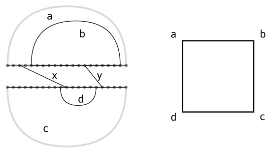
Figure 5. Left: an interaction structure with two interaction arcs, x and y. Right: the corresponding interaction complex.

The inter-molecular arcs naturally induce an equivalence relation $\varphi$ on the vertices of the two backbones. The intersection of two loops is accordingly defined to be the set of $\varphi$-equivalence classes of vertices that they share. A bi-secondary structure can then be viewed as a particular type of interaction structure—namely, an interaction structure with two identical backbones, where interaction arcs connect any pair $(i,i)$ for $0\le i\le n+1$. In contrast to a bi-structure, an interaction structure can exhibit nontrivial first-simplicial homology and requires revisiting the notion of a crossing component for interaction structures. The analysis involves many more topologies—in particular, surfaces and Mayer–Vietoris sequences [34].

The framework of the weighted homology is by no means restricted to bi- or interaction structures. It also gives rise to the consideration of the dissimilarity complex of a finite set of genomic sequences, which we briefly discuss in the following. A multiple sequence alignment W of genomic sequences is defined to be a finite set of words of equal length m over the finite alphabet $A=\{a_1,\cdots ,a_s\}$. For any $k\in \{1,\cdots ,m\}$, let $f_k:W\stackrel{}{\to }A$ be the map that returns the symbol at position k of a word, namely, $f_k(w)=a_{w_k}$ for $w=a_{w_1}\dots a_{w_m}\in W$. A $d+1$ subset $\sigma \subseteq W$ forms a d-simplex if there exists at least one position j such that $\left|\right\{f_j(w)|w\in \sigma \}|=d+1$. In other words, all $d+1$ sequences in $\sigma$ contain mutually different nucleotide types at the site j. For a fixed $\sigma$, the number of different positions j for which the above holds is called the dissimilarity of $\sigma$. This leads to the aforementioned dissimilarity complex for genomic sequences; see Figure 6. This complex is, by definition, low dimensional; its highest dimension is $s-1$. For $d+1=2$, the 1-skeleton of the dissimilarity complex captures the well-known Hamming distance—the number of positions in which two genetic sequences differ. It may be worth pointing out that this framework integrates well-known generalizations of distances, as these appear naturally as weights in the dissimilarity complex. Triangle inequalities generalize to tetrahedron inequalities, etc., and this could enhance our understanding of genetic sequences. This is because basic constructs—e.g., trees, such as the tree of life—that reflect the ancestral relations between sequences depend on the notion of Hamming distance. Our preliminary investigations suggest that the homology of the dissimilarity complex captures evolutionary events. For example, the free rank of the first homology module gives bounds of the possible recombinations within the sequence set.

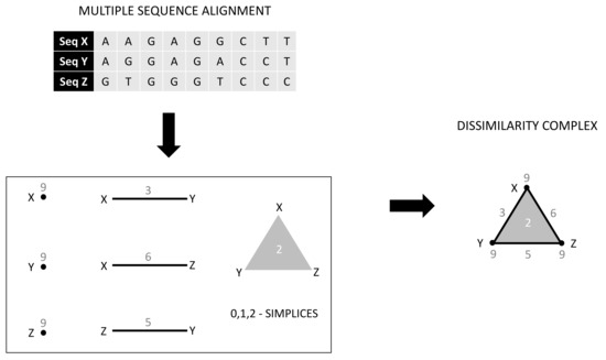
Figure 6. A multiple-sequence alignment of three sequences $X,Y,Z$, their corresponding weighted simplices, and the associated dissimilarity complex.

References

- Bura, A.C.; He, Q.; Reidys, C.M. Loop Homology of Bi-secondary Structures. Discret. Math. 2021, 344, 112371. [Google Scholar] [CrossRef]
- Huang, F.W.; Barrett, C.L.; Reidys, C.M. The energy-spectrum of bicompatible sequences. arXiv 2019, arXiv:1910.00190. [Google Scholar]
- Ren, S.; Wu, C.; Wu, J. Weighted persistent homology. Rocky Mt. J. Math. 2018, 48, 2661–2687. [Google Scholar] [CrossRef]
- Holley, R.W.; Apgar, J.; Everett, G.A.; Madison, J.T.; Marquisee, M.; Merrill, S.H.; Penswick, J.R.; Zamir, A. Structure of a ribonucleic acid. Science 1965, 147, 1462–1465. [Google Scholar] [CrossRef] [PubMed]
- Thirumalai, D.; Lee, N.; Woodson, S.A.; Klimov, D. Early events in RNA folding. Annu. Rev. Phys. Chem. 2001, 52, 751–762. [Google Scholar] [CrossRef]
- Fresco, J.R.; Alberts, B.M.; Doty, P. Some molecular details of the secondary structure of ribonucleic acid. Nature 1960, 188, 98–101. [Google Scholar] [CrossRef] [PubMed]
- Darnell, J.E. RNA: Life’s Indispensable Molecule; Cold Spring Harbor Laboratory Press: New York, NY, USA, 2011. [Google Scholar]
- Chapuy, G. A new combinatorial identity for unicellular maps, via a direct bijective approach. Adv. Appl. Math. 2011, 47, 874–893. [Google Scholar] [CrossRef]
- Waterman, M.S. Secondary structure of single-stranded nucleic acids. Adv. Math. Suppl. Stud. 1978, 1, 167–212. [Google Scholar]
- Schmitt, W.R.; Waterman, M.S. Linear trees and RNA secondary structure. DIscrete Appl. Math. 1994, 51, 317–323. [Google Scholar] [CrossRef]
- Hofacker, I.L.; Schuster, P.; Stadler, P.F. Combinatorics of RNA secondary structures. Discret. Appl. Math. 1998, 88, 207–237. [Google Scholar] [CrossRef]
- Haslinger, C.; Stadler, P.F. RNA structures with pseudo-knots: Graph-theoretical, combinatorial, and statistical properties. Bull. Math. Biol. 1999, 61, 437–467. [Google Scholar] [CrossRef] [PubMed]
- Jin, E.Y.; Qin, J.; Reidys, C.M. Combinatorics of RNA structures with pseudoknots. Bull. Math. Biol. 2008, 70, 45–67. [Google Scholar] [CrossRef] [PubMed][Green Version]
- Orland, H.; Zee, A. RNA folding and large N matrix theory. Nucl. Phys. B 2002, 620, 456–476. [Google Scholar] [CrossRef]
- Andersen, J.E.; Chekhov, L.O.; Penner, R.; Reidys, C.M.; Sułkowski, P. Topological recursion for chord diagrams, RNA complexes, and cells in moduli spaces. Nucl. Phys. B 2013, 866, 414–443. [Google Scholar] [CrossRef]
- Bon, M.; Vernizzi, G.; Orland, H.; Zee, A. Topological classification of RNA structures. J. Mol. Biol. 2008, 379, 900–911. [Google Scholar] [CrossRef] [PubMed]
- Andersen, J.E.; Penner, R.C.; Reidys, C.M.; Waterman, M.S. Topological classification and enumeration of RNA structures by genus. J. Math. Biol. 2013, 67, 1261–1278. [Google Scholar] [CrossRef] [PubMed]
- Huang, F.W.; Reidys, C.M. Shapes of topological RNA structures. Math. Biosci. 2015, 270, 57–65. [Google Scholar] [CrossRef]
- Chen, W.; Deng, E.; Du, R.; Stanley, R.; Yan, C. Crossings and nestings of matchings and partitions. Trans. Am. Math. Soc. 2007, 359, 1555–1575. [Google Scholar] [CrossRef]
- Stanley, R.P. Enumerative Combinatorics; Wadsworth Publ.: Belmont, CA, USA, 1986. [Google Scholar]
- Sundaram, S. The Cauchy Identity for sp (2n). J. Comb. Theory Ser. A 1990, 52, 209–238. [Google Scholar] [CrossRef]
- Penner, R.; Waterman, M.S. Spaces of RNA secondary structures. Adv. Math. 1993, 101, 31–49. [Google Scholar] [CrossRef]
- Zuker, M.; Sankoff, D. RNA secondary structures and their prediction. Bull. Math. Biol. 1984, 46, 591–621. [Google Scholar] [CrossRef]
- Gralla, J.; Crothers, D.M. Free energy of imperfect nucleic acid helices: II. Small hairpin loops. J. Mol. Biol. 1973, 73, 497–511. [Google Scholar] [CrossRef]
- Turner, D.H.; Mathews, D.H. NNDB: The nearest neighbor parameter database for predicting stability of nucleic acid secondary structure. Nucleic Acids Res. 2009, 38, D280–D282. [Google Scholar] [CrossRef] [PubMed]
- Nussinov, R.; Jacobson, A.B. Fast algorithm for predicting the secondary structure of single-stranded RNA. Proc. Natl. Acad. Sci. USA 1980, 77, 6309–6313. [Google Scholar] [CrossRef]
- Waterman, M.S.; Smith, T.F. Rapid dynamic programming algorithms for RNA secondary structure. Adv. Appl. Math. 1986, 7, 455–464. [Google Scholar] [CrossRef]
- McCaskill, J.S. The equilibrium partition function and base pair binding probabilities for RNA secondary structure. Biopolym. Orig. Res. Biomol. 1990, 29, 1105–1119. [Google Scholar] [CrossRef]
- Reidys, C.M. Random induced subgraphs of generalizedn-cubes. Adv. Appl. Math. 1997, 19, 360–377. [Google Scholar] [CrossRef][Green Version]
- Flamm, C.; Hofacker, I.L.; Maurer-Stroh, S.; Stadler, P.F.; Zehl, M. Design of multistable RNA molecules. RNA 2001, 7, 254–265. [Google Scholar] [CrossRef]
- Bura, A.C.; He, Q.; Reidys, C.M. Loop homology of bi-secondary structures II. arXiv 2019, arXiv:1909.01222. [Google Scholar]
- Whitehead, J. Simplicial Spaces, Nuclei and m-Groups. Proc. Lond. Math. Soc. 1939, 2, 243–327. [Google Scholar] [CrossRef]
- Cohen, M.M. A Course in Simple-Homotopy Theory, 2nd ed.; Springer: Berlin, Germany, 1973. [Google Scholar]
- Hatcher, A. Algebraic Topology; Cambridge University Press: Cambridge, UK, 2000. [Google Scholar]
- Andersen, J.E.; Huang, F.W.; Penner, R.C.; Reidys, C.M. Topology of RNA-RNA interaction structures. J. Comput. Biol. 2012, 19, 928–943. [Google Scholar] [CrossRef] [PubMed]
Publisher’s Note: MDPI stays neutral with regard to jurisdictional claims in published maps and institutional affiliations. |
© 2021 by the authors. Licensee MDPI, Basel, Switzerland. This article is an open access article distributed under the terms and conditions of the Creative Commons Attribution (CC BY) license (https://creativecommons.org/licenses/by/4.0/).