Abstract
This paper presents a study on the optimization problem of a consumer’s choice constrained to a single time interval. In this problem, the choice is made over a set of perishable goods such that they do not retain value at the end of the period. Money has been introduced as the only means available to store that value for the future. Thus, consumer utility is measured on the possible combinations of goods consumed during the period and money held at the end of the period. Additionally, a set of simple conditions are assumed to the utility functions for goods and money given by: (1) Existence of a total utility that is additively separable with respect to the components of goods and money; (2) continuity of the derivatives of the utility functions of money and goods up to the second degree; and (3) non-uniqueness of the matrix obtained by differentiating the system of equations obtained by the condition of optimum. The article shows how the requirement of homogeneity conditions limits the possible expressions for the utility function of money. One of them is the frequently used logarithmic function.
1. Introduction
The nature of money in economic analysis has been subjected to wide discussions, as it is developed in [1,2]. Following the considerations of Hicks [3], the concept of money must be defined through its functions that are generally resumed in the following three points: mean of payment, measure of value, and a mean of store value. This definition contains a point of incompleteness that has been the origin of some controversies.
Its inclusion in optimization models has been studied in a large number of research papers. The different approaches have been the subject of debate and controversy (see for example [4]). Another interesting summary of the topic, with an explanation of the problem of the exogenous character of money in Walrasian models is [5].
From the point of view of the justification of money in the economy, it is generally considered to be a means of transferring resources between different time intervals. Development of these kind of models, called Money in Utility (MIU), has been extensive, considering different types according to the assumptions on which they are based (see again [5] for a summary). As a short list, we could introduce the model of overlapping generations (Samuelson [6]), the works of Clower [7]; Lucas [8,9,10]; Lucas and others [11]; and also the models of Patinkin [12], Sidrauski [13], or Hansen [14]. Derivations and simplifications of these models can be found in [1,4,15].
With regard to the characteristics of the utility function of money in these models, it is often assumed that the utility of consumer goods and money can be separated through additive terms (see by example [16]).
Theory of decision under uncertainty includes money in the utility function in a natural way, because the related problems are usually presented in terms of money as the output of the considered options. A model of utility that can be frequently found by example in [17,18,19] is that given by:
where r is the constant relative risk aversion for money. So, , and imply risk preference, risk neutrality and risk aversion respectively. In the limit case the expression is redefined using the logarithm:
Logarithmic expressions for money utility have a long tradition in uncertainty studies because of its good properties. However, there is no unique approach in these fields, as can be seen in [20].
The main purpose of the present research is to study whether somehow the functional form of with respect to the variable under consideration (money in this case) can be justified from some set of conditions on the properties of the utility functions.
There is a variety of utility functions that are used in research and that are selected or proposed on the basis of their properties and mathematical behavior. The question we have tried to study (albeit partially since it only concerns money as a good) is whether somehow some of these functions could be determined by the conditions that are usually assumed in utility maximization problems.
2. Materials and Methods
2.1. Flows of Goods and Money. Perishable Goods
Let us consider a good that is available in the market for the consumer, and let us denote as the amount of good at the beginning of the i-th time interval. Consider the flow during this interval as shown in Figure 1.
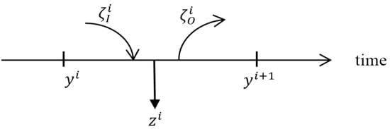
Figure 1.
Flow of goods.
Then, the value of this variable at the end of the interval (and the beginning of the (i + 1)-th interval) can be written as:
where and represent the input and output flows of the good in the interval, and accounts for its depreciation or consumption. Supposing that in an interval any good will only be bought or sold, the variables and can be grouped in a new one:
And Equation (1) takes the form:
In the case of money, the flow is represented in Figure 2:
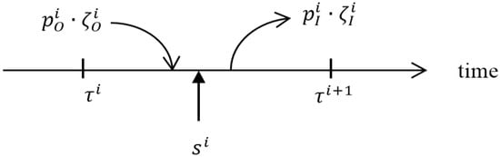
Figure 2.
Flow of money.
Then, representing as the quantity of money at the beginning of the i-th interval, the flow is now:
The terms in Equation (4) can be reordered in a way that gives a direct meaning to the involved terms:
Here represents the maximum amount of money available for the consumer including that obtained selling the durable goods held at the beginning of the interval.
To simplify the problem is interesting in the case of considering only the case of perishable goods. This constraint is especially useful to highlight the nature of money in the model, because there is no other alternative to transfer wealth between periods than the money itself. In this case, during any considered interval, all the amount of good will vanish, so . Taking this to Equation (1):
If the good will not be available at the next period of time, it has no sense to consider its sale for the consumer, so Equation (6) simplifies as:
Considering the flow of money, apart from the non-perishable goods, Equation (5) can be written as:
where is the maximum amount of available liquid money in the interval without considering incoming flows obtained by selling goods.
Introducing the vector as the consumed amount of good in the i-th interval, in the perishable case . And so, the final version of Equations (1) and (4) are:
and:
2.2. Money in Utility Model for a Market of Perishable Goods
Let us consider the expression of a MIU model in a single interval. In the case of perishable goods, the consumer will evaluate the amount consumed or bought during the interval, denoted by the variable x. With respect to money, the consumption decision will have in account the final amount of available money, denoted by . The model for MIU will have then the form [13]:
Supposing additive separability for goods and money, Equation (11) takes the form:
Being W the utility of money and V the utility of the set of perishable goods.
Equation (13) represents the problem of maximization of the function under the constraint given by Equation (10). As the problem involves only one period, superscripts can be ignored:
The solution for this problem is given by the system:
Without assumptions on the properties of the utility functions, the conditions given by Equation (14) are only necessary conditions.
Following, a comparative static analysis will be made on the solution. Deriving the system of equations:
Reordering terms, for expressing the dependence of on :
Or in matrix form:
Let us consider the matrix that corresponds to the hessian of the constrained utility , where ⊗ is the tensorial product operator. If its determinant is non-zero (a sufficient condition for the existence of a maximum implies among other things, that condition), it will have an inverse that can be calculated by blocks:
where the matrix Ω is:
Multiplying by the left Equation (17) with the matrix in Equation (18):
Expression (20) can be written in terms of income and substitution effects:
2.3. Homogeneity Conditions and Consequences
Under a transform in the monetary unit , the constraint of Equation (13) changes as:
Imposing invariance of the problem under this transform, it must be:
From the condition of homogeneity on x:
But using Equation (20) this implies:
Equation (25) is satisfied under different cases:
Case 1. for every α seems to be a too hard a condition over any arbitrary set of goods and prices.
Case 2. would imply that , and Equation (20) takes the form:
As a consequence, any change in with no changes in prices would not affect the selected basket. This result seems not very realistic except in the case of values of m that in practice do not allow to select any basket, that is for very poor people there is no change between having one or five monetary units if the cost of the cheapest product is by example 500. Clearly, the needs of this kind of consumer must be satisfied by using ‘alternative circuits’ other than the normal market.
Case 3. implies an expression for the function W: .
Logarithmic expressions for utility money appear in several papers, and it is widely used in research about decisions under uncertainty. However, no justification for this form is usually presented to further its simplicity and custom.
Now, Equation (21) would be:
Now, the marginal value of money is:
On the other side, the selected basket will provide a greater utility than maintaining all the money, so:
From here, a lower bound for the selected goods can be derived from the saving fraction:
From the results obtained in cases (2) and (3), the next function for the utility of money can be proposed:
With , a logistic-like function that introduces a smooth transition between the two regimes from a reference point . A significant amount of scientific work refers to this concept of ‘poverty line’ with interesting discoveries and conclusions, see by example in [21] and beyond and related with this, concepts as the poverty trap are related with different preferences of the consumers with respect to risk with implications on the convexity of the utility function on both sides of a critical income (see [22,23]). These results are in accordance with the more general dependence between wealth and absolute and relative risk aversions, by example [24,25].
The plot of function defined in (31) is shown in Figure 3:
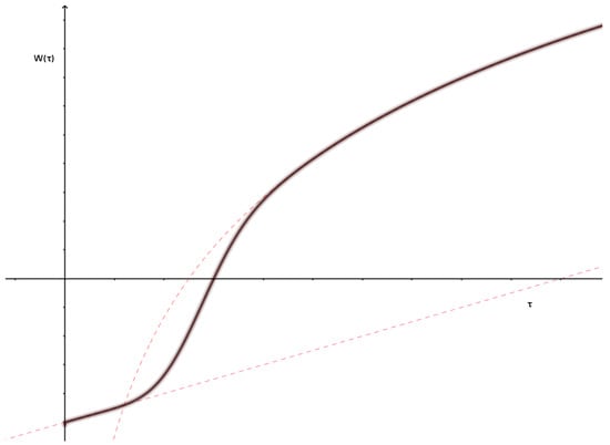
Figure 3.
S-Shaped utility function of money.
S-Shaped utility functions for money like this have been considered by example in [20].
3. Discussion
In basic microeconomic theory of consumer behaviour optimisation, money acts as a constraint on the available consumption basket. However, the inclusion of money within the utility function is common in consumption optimisation problems over various time intervals. Another field of study in which it frequently appears as an argument of a utility function is in the theory of consumption decisions under uncertainty.
The use of logarithmic expressions for the utility function of money is extensive and widespread. However, a justification for this choice is not easily found in the available literature. This paper presents a development that leads to the need for such an expression for the utility of money based on the following minimum assumptions, which are in no way restrictive or demanding. Namely:
- Introduction of money into the utility function as an additional good. The utility derived from the possession of such a good can be assumed, as is done in a large part of the literature, as a means of preserving the current capacity to consume and transferring it to future periods. The fact that these periods are not explicitly considered in the utility function does not imply the invalidity of such utility.
- Optimization of consumer utility over a single period in a market for perishable goods. Regardless of whether the money can be used later, the optimization model focuses only on the decisions to be made in a given time interval. In this case, the variables on which the consumer can decide are the amount of goods he consumes and the money he does not spend. Not considering durable goods implies that the only way of storing value between periods is money.
- conditions are assumed for the utility functions of goods and money and the invertibility of the differential of the equilibrium equations. These conditions are not demanding and are usually considered in classical models of optimization of consumer behavior, where properties such as monotony and cuasi-concavity are generally taken for granted, producing equivalent results.
The main result of this paper is the restriction imposed by Equation (25) on the function W. As a consequence, only two expressions are allowed for , the linear and the logarithmic. The second one has been frequently used in the literature. However, there exists a problem with the meaning of its behaviour at the origin. For that reason, as a hypothesis, the authors propose a form of joining these two expressions on a ‘global . However, this is only wishful thinking because the function introduced in Equation (31) can present problems (by example, the maintenance of homogeneity around ) that should be studied more in depth in the future.
Author Contributions
Formal analysis, F.J.N.-G. and Y.V.; Investigation, F.J.N.-G.; Writing—original draft, F.J.N.-G.; Writing—review & editing, Y.V. All authors have read and agreed to the published version of the manuscript.
Funding
This research received no external funding.
Institutional Review Board Statement
Not applicable
Informed Consent Statement
Not applicable
Data Availability Statement
Not applicable
Conflicts of Interest
The authors declare no conflict of interest.
References
- Asada, T. Money in Economic Analysis. In Mathematical Models in Economics-Volume II; EOLSS Publications: Paris, France, 2010; p. 112. [Google Scholar]
- Toledo, W. El dinero en los modelos macroeconómicos. Rev. de Econ. Inst. 2006, 8, 97–116. [Google Scholar]
- Hicks, J.R. Critical Essays in Monetary Theory; Clarendon Press: Oxford, UK, 1967; p. 219. [Google Scholar]
- Feenstra, R.C. Functional equivalence between liquidity costs and the utility of money. J. Monet. Econ. 1986, 17, 271–291. [Google Scholar] [CrossRef]
- Bridel, P. Patinkin, Walras and the 'money-in-the-utility-function’ tradition. Eur. J. Hist. Econ. Thought 2002, 9, 268–292. [Google Scholar] [CrossRef]
- Samuelson, P.A. An Exact Consumption-loan of Interest with or without the Social Contrivance of Money. J. Polit. Econ. 1958, 66, 467–482. [Google Scholar] [CrossRef]
- Clower, R.W. A Reconsideration of Microfoundations of Monetary Theory. In Money and Markets: Essays by Robert Clower; Walker, D.A., Ed.; Cambridge University Press: Cambridge, UK, 1967; pp. 81–89. [Google Scholar]
- Lucas, R. Expectations and the Neutrality of Money. J. Econ. Theory 1972, 4, 103–124. [Google Scholar] [CrossRef]
- Lucas, R. Equilibrium in Pure Currency Economy. In Models of Monetary Economics; Kareken, J.H., Wallace, N., Eds.; Federal Reserve Bank of Minneapolis: Minneapolis, MN, USA, 1980; pp. 131–146. [Google Scholar]
- Lucas, R. Models of Business Cycles; Basil Blackwell: Oxford, UK, 1987. [Google Scholar]
- Lucas, R.E., Jr.; Stokey, N.L. Money and Interest in a Cash in Advance Economy. Econometrica 1987, 55, 491–514. [Google Scholar] [CrossRef]
- Patinkin, D. Money, Interest and Prices; Harper & Row: New York, NY, USA, 1965. [Google Scholar]
- Sidrauski, M. Rational choice and patterns of growth in a monetary economy. Am. Econ. Rev. 1967, 57, 534–544. [Google Scholar]
- Hansen, B. A Survey of General Equilibrium System; McGraw-Hill: New York, NY, USA, 1970. [Google Scholar]
- Irgoin, C.A. Modelo Money in Utility Function (Miu); Contribuciones a la Economía: País, Spain, 2010. [Google Scholar]
- Fukuda, S.I. The role of monetary policy in eliminating non-convergent dynamic paths. Int. Econ. Rev. 1997, 38, 249–261. [Google Scholar] [CrossRef]
- Pratt, J.W. Risk aversion in the small and in the large. Econometrica 1964, 32, 122–136. [Google Scholar] [CrossRef]
- Arrow, K.J. Aspects of a Theory of Risk Bearing, Yrjo Jahnsson Lectures, Helsinki; Reprinted Frontiers in Human Neuroscience in Essays in the Theory of Risk Bearing; Markham Publishing Co.: Chicago, IL, USA, 1965. [Google Scholar]
- Holt, C.; Laury, S. Risk aversion and incentive effects. Am. Econ. Rev. 2002, 92, 1644–1655. [Google Scholar] [CrossRef]
- Bosch-Domènech, A.; Silvestre, J. Does risk aversion or attraction depend on income? An experiment. Econ. Lett. 1999, 65, 265–273. [Google Scholar] [CrossRef]
- Seidl, C. Poverty measurement: A survey. In Welfare and Efficiency in Public Economics; Springer: Berlin/Heidelberg, Germany, 1988; pp. 71–147. [Google Scholar]
- Just, D.R.; Michelson, H.C. Wealth as welfare: Are wealth thresholds behind persistent poverty? Rev. Agric. Econ. 2007, 29, 419–426. [Google Scholar] [CrossRef]
- Yesuf, M.; Bluffstone, R.A. Poverty, risk aversion, and path dependence in low-income countries: Experimental evidence from Ethiopia. Am. J. Agric. Econ. 2009, 91, 1022–1037. [Google Scholar] [CrossRef]
- Paravisini, D.; Rappoport, V.; Ravina, E. Risk aversion and wealth: Evidence from person-to-person lending portfolios. Manag. Sci. 2017, 63, 279–297. [Google Scholar] [CrossRef]
- Heinemann, F. Measuring risk aversion and the wealth effect. Res. Exp. Econ. 2008, 12, 293–313. [Google Scholar]
Publisher’s Note: MDPI stays neutral with regard to jurisdictional claims in published maps and institutional affiliations. |
© 2021 by the authors. Licensee MDPI, Basel, Switzerland. This article is an open access article distributed under the terms and conditions of the Creative Commons Attribution (CC BY) license (http://creativecommons.org/licenses/by/4.0/).