Passive Strategies to Improve the Comfort Conditions in a Geodesic Dome

Abstract

Non-conventional thermal zones are low-cost and ecology friendly alternatives to the housing needs of populations in various situations, such as surviving natural disasters or addressing homelessness. However, it is necessary to guarantee thermal comfort for occupants, while aiming to minimize energy consumption and wastage in refrigeration systems. To reduce the cooling requirements in non-conventional thermal zones it is necessary to model the structure and analyze the principal factors contributing to internal temperature. In this paper, a geodesic dome is modellingusing the lumped parameter technique. This structure is composed of a wooden skeleton and wooden floor, with a canvas surface as its exterior. The mathematical model was tuned using experimental data, and its parameters were classified using Monte Carlo sensitivity analysis. The mathematical model was used to evaluate the impact on internal temperature and occupants’ comfort when two strategies are considered. The results obtained indicatee internal temperature reductions down to a range of 7% to 11%; this result is reflected directly in the energy used to refrigerate the thermal zone, contributing to the objective of providing houses with lower energy consumption.

1. Introduction

The 21st century presents a series of challenges for the current society, such as global warming, depletion of natural resources, and satisfying the requirements of the world population without destroying ecosystems. As a response to these problems, the sustainable development goals were adopted by the member countries of the United Nations (UN) in 2015 [1]. The objectives include inclusive, safe, resilient, and sustainable cities. This is a very difficult goal to fulfill with the increasing growth of the world population, as the more people live in cities, the more resources and energy are needed.

The formulation of the sustainable development goals has affected different research fields, especially those related to reducing the energy consumption in residential buildings [2,3,4]. Energy consumption depends on various factors, such as the nature of the electronic equipment, the number of occupants, the level of activity and the degree of comfort. The last aspects are directly related to the use of heat ventilation air-conditioning (HVAC) systems. The HVAC can represent more than 40% of the energy consumption in buildings [5,6,7], which means that any reduction in the use of air conditioning systems can seriously impact the world energy expenditure.

The scientific literature relates different strategies to minimize the use of air-conditioned systems, which is especially high in tropical countries and during the spring season in countries in temperate zones [8,9,10]. Regularly, these strategies have focused on minimizing the heat flux transfer between buildings and the environment. These strategies are classified as passive strategies and are characterized by the introduction of modifications in the exterior surfaces of the buildings [11,12,13].

The use of green roofs is a passive strategy which is one of the most ancient and frequent technique for minimizing the incoming heat from the exterior, probably because it includes additional environmental benefits such as the oxygen production and runoff water reduction [14,15]. The strategy is based on using vegetation layers over rooftops and walls, taking advantage of the natural ability of plants to process solar radiation, allowing them to function as a thermal barrier [16]. This strategy can be combined with other strategies such as a photovoltaic rooftop that enhances the capabilities of solar panels [17,18]. Another important strategy is the use of a coating of thermal paint, which is known as a cold roof. The use of coating paints in rooftops and walls reduces the incoming heat and directly affects the amount of energy required for cooling [19,20]. Experimental and theoretical research carried out in buildings demonstrate that a thermal coating reduces the internal air temperature by 2.3 °C [21]. In laboratory tests reported in [22], a saving of up to 2.9% was obtained. However, even though these results are promising, new types of insulating materials are constantly being developed [23,24]. This is the case with the new thermal coating being tested in reduced scale models at the Universitat Politècnica de València, Spain. The study yielded reductions of interior temperatures by 7.4% [25].

All these passive strategies can be used to reduce the interior temperature, but one drawback is that in many cases it is not possible to carry out experimental evaluations of multiple thermal coatings, such as in [26], where different products were tested in building facades. An important alternative is to run thermal models to test the impact of passive strategies. Any good mathematical model should be adjusted to real conditions to allow accurate results [3].

The mathematical modeling of thermal zones is important prior to experimental tests of HVAC. For example, in [21], the model was tuned for the specific conditions in a given place and reused for two additional locations. This kind of tests allows for the selection of the best solution for different places with similar conditions, or different kinds of thermal zones and buildings. In [27] a thermal network was used to study the impact of different loads on energy consumption in a building. The model was adjusted to predict the electrical behavior of a campus in Naval Station Great Lakes, Illinois. The investigation presented in [28] studied the thermal response of different structures, such as roofs and decks, which can provide an important heat gain for the solar radiation absorbed. In general, there is plenty of published work on the thermal behavior of buildings, but most are dedicated to traditional structures such as rectangular buildings, which do not consider non-conventional structures and their possible use for low energy consumption [29,30,31].

Different strategies for building modeling have been reported in the literature [32,33,34,35]; each one has advantages and disadvantages. In many cases, the selected strategy is determined by the structure to be studied and by the research capacities [36,37,38]. To reduce the complexity during the construction of the mathematical model, many engineers use simple and adaptable techniques, such as the lumped parameters strategy [39,40,41]. This technique uses an analogy with RC circuits (resistor and capacitor) and, using Kirchhoff’s laws, a thermal model for the studied building can be established. This technique allows users to configure the circuit to study different structures with multiple wall layers [42,43,44].

The present work aims to evaluate an autochthonous habitat’s adequate behavior in response to the daily thermal oscillation, which was monitored in the mountainous region near Santa Marta. The autochthonous habitat is characterized by a low form factor in its construction (surface/volume ratio) and materiality with low transmission values, due to the use of highly insulating plant fibers. Given the difficulty of reproducing an autochthonous habitat at present, we chose to work on a model that essentially reproduced its thermodynamic behavior. Our model involved two essential elements: a geodesic dome as a form due to the closeness of its form factor to those of vernacular architectures, and a heat-insulating coating that simulated the behavior of the vegetable fibers that make up these enclosures. In this respect, the analysis of a non-conventional thermal zone, namely, a geodesic dome, is presented. The study focusses on modeling the structure and on evaluating the impact on the interior temperature using passive strategies. The goal was to show that by introducing modifications to the envelopem the internal temperature can be reduced, thus minimizing the energy requirements for refrigeration for the habitability of the thermal zone. The article is organized as follows: the second section is dedicated to presenting the mathematical model and its physical and geometric parameters; in the third section, the model is tuned with experimental data and used to analyze the principal factors to guarantee the occupant’s comfort; in the fourth section, the impact of passive strategies and adaptations to the dome on the internal temperature are evaluated; and finally, in the fifth section, some conclusions are drawn.

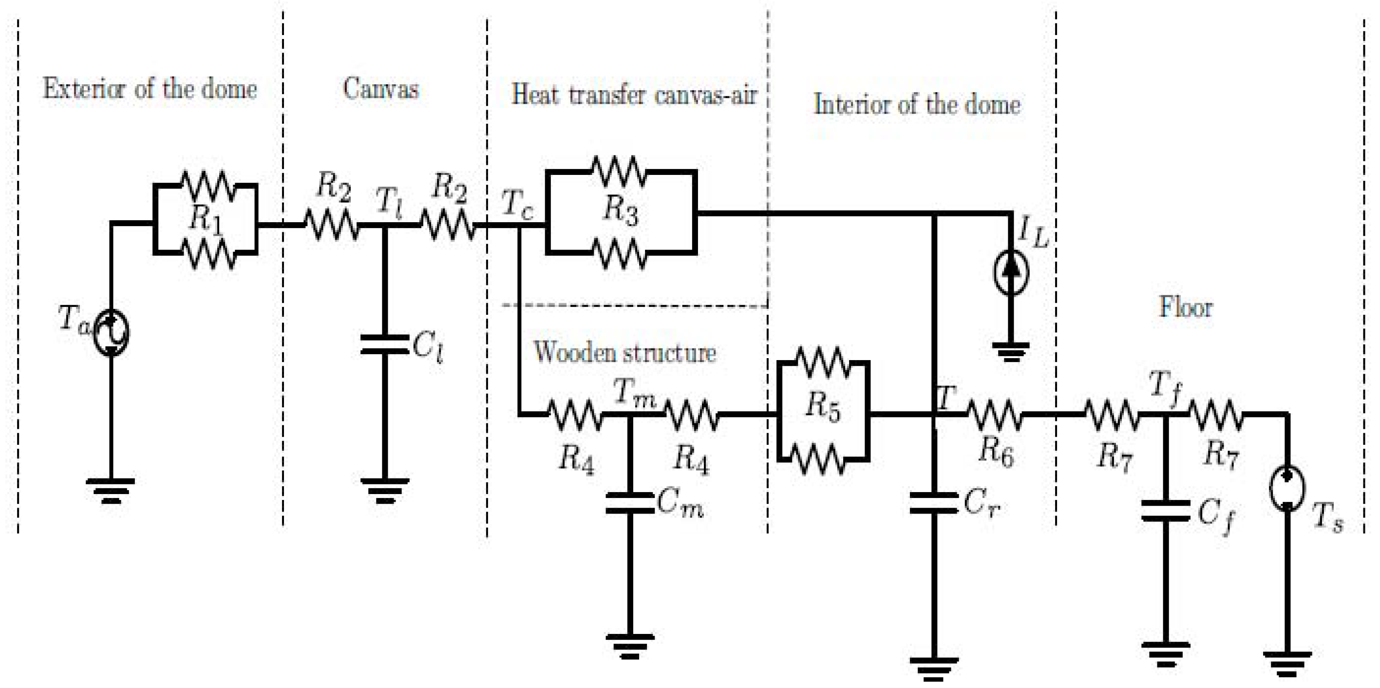
2. Modeling a Geodesic Dome

The structure chosen in this work was a geodesic dome built in the Universidad del Magdalena (Colombia). The geodesic dome was modeled from a truncated icosahedron, on whose faces pyramids were built, with their bases on the faces of the polyhedron, and with its vertex on the circumscribed sphere.

The thermal zone had a wooden floor as a base, a wooden structure, and a canvas for the external surface. Figure 1 shows the internal structure of the dome and some of the geometrical data. The left and central pictures show different views of the internal structure, and the right picture shows its building process. Each triangle was formed by wooden segments with dimensions $1.2 \mathrm{m}\times 0.1 \mathrm{m}\times 0.025 \mathrm{m}$.

The geodesic dome was modeled and studied using the lumped parameter strategy. Figure 2 represents a cross-section of the dome and shows the internal structure of the thermal zone. This picture also introduces the variables considered in the model, which are the canvas temperature ($T_l$), the wooden structure temperature ($T_m$), the floor temperature ($T_f$), and the internal air temperature ($T$). Additionally, in Figure 2 other variables are indicated, that is, the environmental temperature ($T_a$), the ground temperature ($T_s$), the superficial external and internal canvas temperature ($T_{sle}$ and $T_{sli}$), the superficial wooden structure temperature ($T_{sm}$), and the superficial floor temperature ($T_{sf})$. Finally, the internal loads are represented by $I_L$, and the heat flux transferred by the canvas and the wooden structure ($Q_l$ and $Q_m$) correspond to the incoming heat flux ($Q_i)$.

This thermal zone was studied in [45], where a previous version of the mathematical model was presented, which is updated here to include two new aspects. The first modification is the ability to consider the heat transfer by radiation and convection individually. The second aspect is related to using the floor temperature as a state variable. These modifications provide a more accurate mathematical model, according to the circuit diagram used in the literature [39]. Figure 3 shows the circuit diagram used to represent the geodesic dome. This circuit shows the different zones, elements, and heat process in the dome. The resistors and capacitors are calculated according to the physical parameters of the dome. The parameters used are the surface area ($A$), thickness ($L$), thermal conductivity ($kt$), density ($\rho$) and specific heat ($Ce$). In the rest of the article the subscripts l, m, f and a are used to indicate the element to which each parameter belongs. The subscript l stands for canvas, m for wooden structure, f for floor, and finally, the subscript a stands for air.

Table 1. Geometric and physical parameters.

Feature\Element	Canvas	Wooden Structure	Floor	Air
Superficial area $({\mathrm{m}}^2$)	$56.54$	$2.82$	$9\pi$	$NA$
Thickness $(\mathrm{m}$)	$56\times {10}^{-4}$	$0.10$	$0.4$	$NA$
Thermal conductivity $(\mathrm{W}/\left(\mathrm{m}·\mathrm{K}\right)$)	$0.15$	$0.21$	$0.19$	$0.025$
Specific heat $\left(\mathrm{kJ}/\left(\mathrm{kg}·°\mathrm{C}\right)\right)$	$1.05$	$2.51$	$2.51$	$1.0$
Density $\left(\mathrm{kg}/{\mathrm{m}}^3 \right)$	$895.50$	$640$	$555.50$	$1.2$

shows the values for each physical and geometric parameter.

In the case of the internal air, it is not possible to use superficial area and thickness; instead we used the internal volume $V_i=146 {\mathrm{m}}^3$. According to Figure 3, the exterior of the dome includes the environmental temperature and $R_1$ resistors, which are used to represent the opposition of the canvas’ external surface to transfering heat with convection and radiation process. The two resistors represent the heat transfer processes between the air and the wood or canvas surface. When a single resistor is used, it represents the conduction process.

$R_1$ is calculated in Equation (1) using $h$ and $\epsilon$ as convection and radiation coefficients for the external surface. These coefficients must be adjusted to environmental conditions to obtain an accurate simulation. Similarly, Equations (3), (5) and (6) represent the convection and radiation resistances for the surfaces on the interior dome, specifically, the canvas’ internal surface, the wooden structure, and floor. It is necessary to remark that the coefficient division is one of the improvements in this model which allows for a better characterization of the heat flux process. Previously, the transference between surface and air was handled with one single coefficient. Now, by using two independents coefficients it is possible to evaluate the impact of each and implement solutions directly over one heat transfer process.

Equations (2), (4) and (7) represent the resistance to the conduction heat process in the canvas, wood structure, and floor, respectively. The parameters used in these expressions, such as the thermal conductivity and superficial area are measured or taken from the literature [46].

$$R_1=\frac{1}{A_l\left(h_{le}+{\epsilon }_{le}\sigma \left(T_{sle}+T_a\right)\left(T_{sle}^2+T_a^2\right)\right)}$$

(1)

$$R_2=\frac{L_l}{2k{t}_l{A}_l}$$

(2)

$$R_3=\frac{1}{A_l\left(h_{li}+{\epsilon }_{li}\sigma \left(T_{sli}+T\right)\left(T_{sli}^2+T^2\right)\right)}$$

(3)

$$R_4=\frac{L_m}{2k{t}_m{A}_m}$$

(4)

$$R_5=\frac{1}{A_m\left(h_m+{\epsilon }_m\sigma \left(T_{sf}+T\right)\left(T_{sf}^2+T^2\right)\right)}$$

(5)

$$R_6=\frac{1}{A_f\left(h_f+{\epsilon }_f\sigma \left(T_{sf}+T\right)\left(T_{sf}^2+T^2\right)\right)}$$

(6)

$$R_7=\frac{L_f}{2k{t}_f{A}_f}$$

(7)

The constants $C_l, C_m, C_f,$ and $C_r$ represent the capacity of each element to store thermal energy and were taken from [45].

The mathematical model is presented in Equations (8)–(11), using canvas, wooden structure, floor, and internal air temperatures as state variables. Sources $T_a$ and $T_s$ are used to represent the environmental and ground temperatures. The current source $I_L$ represent all the internal gains in the system, such as occupants, electronic equipment, refrigeration systems, and the solar gain by skylight. Finally, $T_c$ is the canvas limit temperature, which is calculated in Equation (12).

$$C_l\dot{T_l}=\frac{T_a}{R_1+R_2}-T_l\left(\frac{1}{R_1+R_2}+\frac{1}{R_2}\right)+\frac{T_c}{R_2}$$

(8)

$$C_m{\dot{T}}_m=\frac{T}{R_4+R_5}-T_m\left(\frac{1}{R_4+R_5}+\frac{1}{R_4}\right)+\frac{T_c}{R_4}$$

(9)

$$C_f{\dot{T}}_f=\frac{T_s}{R_7}-T_f\left(\frac{1}{R_6+R_7}+\frac{1}{R_7}\right)+\frac{T}{R_6+R_7}$$

(10)

$$C_r\dot{T}=\frac{T_m}{R_4+R_5}+\frac{T_f}{R_6+R_7}-T\left(\frac{1}{R_4+R_5}+\frac{1}{R_6+R_7}+\frac{1}{R_3}\right)+\frac{T_c}{R_3}+I_L$$

(11)

$$T_c=\frac{R_3{R}_4}{R_2{R}_3+R_2{R}_4+R_3{R}_4}{T}_l+\frac{R_2{R}_4}{R_2{R}_3+R_2{R}_4+R_3{R}_4}T+\frac{R_2{R}_4}{R_2{R}_3+R_2{R}_4+R_3{R}_4}{T}_m$$

(12)

It should be pointed out that the internal loads $I_L$ can change according to the quantity and kind of elements inside the dome; in other words, the internal load can take the form $I_L=N·Q_0+M·Q_e-u·Q_c+Q_v$, using $N$ and $M$ to represent the number of human occupants and electronic equipment working inside the dome, respectively. $Q_o$, $Q_e$ and $Q_v$ are the heat gain by occupants, electronic equipment, and the skylight, respectively; and finally, $Q_c$ is the heat extracted by the cooling system and $u$ is a binary variable used to define the equipment state, $u=1$ for on and $u=0$ for off. In this work, the dome was considered completely empty; thus, $I_L=Q_v$.

3. Tuning and Analysis of Mathematical Model

The model was adjusted using a database recorded for 5 days, from February 9 to 14, 2019, in Santa Marta city (Colombia) [30]. In this database, the internal and external surface temperatures, environmental temperature, and internal air temperature were registered. Other environmental conditions, such as ground temperature (used in Equation (10)), solar radiation, and wind speed were taken from departmental institutions data [31].

The algorithm used for the tuning was PatternSearch. This algorithm is part of the Optimtool toolbox of Matlab, taking as the optimization function the expression $F=\frac{1}{N}\sqrt{{{\displaystyle \sum }}_{i=1}^N{\left(T_i-{\left(T_{exp}\right)}_i\right)}^2}$, using $T_{exp}$ to represent the experimental temperature recorded at the point $i$, and $T$ for the simulated temperature at this point [30]. The procedure for adjustion consists in separating the studied period in the day and night and calculating the best value to fit the simulation curves to the experimental data. This method has been tested in similar investigations [25,47].

The tuned coefficients are presented in

Table 2. Convection and radiation coefficient tuned.

Coefficient/Parameter	${\mathit{h}}_{\mathit{m}}\left[\frac{\mathit{k}\mathit{J}}{\mathit{h}\mathit{·}\mathit{m}\mathit{·}\mathit{K}}\right]$	${\mathit{\epsilon }}_{\mathit{m}}$	${\mathit{h}}_{\mathit{l}\mathit{i}}\left[\frac{\mathit{k}\mathit{J}}{\mathit{h}\mathit{·}\mathit{m}\mathit{·}\mathit{K}}\right]$	${\mathit{\epsilon }}_{\mathit{l}\mathit{i}}$	${\mathit{h}}_{\mathit{l}\mathit{e}}\left[\frac{\mathit{k}\mathit{J}}{\mathit{h}\mathit{·}\mathit{m}\mathit{·}\mathit{K}}\right]$	${\mathit{\epsilon }}_{\mathit{l}\mathit{e}}$	${\mathit{h}}_{\mathit{f}}\left[\frac{\mathit{k}\mathit{J}}{\mathit{h}\mathit{·}\mathit{m}\mathit{·}\mathit{K}}\right]$	${\mathit{\epsilon }}_{\mathit{f}}$
Day	138.8	0.9	67.57	0.9	116	0.9	0.55	0.9
Night	83.3	0.99	8.45	0.01	83.3	0.99	0.27	0.01

. Based on the tuning strategy described, it was possible to obtain a very low percentage difference between the simulation and the experimental data for the day studied. However, using the same parameters for other days can increase the simulation error. In this case, we obtained an error for the studied day of 2.5%, and an error for the rest of days of 3.2%.

Figure 4 depicts the internal simulated temperature with a blue line, the experimental internal temperature with a red line, and the environmental temperature with a green line. The variations in environmental temperature explain the increase in the percentage difference between the experiment and the simulation, because the temperature in later days was greater by 10% than the first-day temperature, which was used to adjust the model.

Figure 5 shows the behavior of canvas temperature ($T_l$), wooden structure temperature ($T_m$), and floor temperature ($T_f$). The blue line is used for canvas temperature, the red line for wooden structure, and the green line for the floor temperature. There are noticeable differences between $T_l$, $T_m$ and $T_f$. The first two are directly related to environmental conditions and the fast variations in T_a, whereas $T_f$ is related to the ground temperature, $T_s$, which was not measured. To overcome this situation, we used $T_s=28.3 \mathrm{°}\mathrm{C}$, which corresponds with the mean annual temperature in the city [48].

Using the tuned mathematical model, we can analyze different aspects such as the incoming heat flux from the exterior, and the impact of each parameter over the internal temperature. The incoming flux is represented by $Q_l$ and reaches the interior air by two different routes. The first route is the energy transfer to the canvas, followed by transfer to the wooden structure, and finally to the interior air. The heat flux that occurs in this way is designated by $Q_m$. The second route uses the gaps between the branches in the wooden structure. The transfer process is from the external air to the canvas, and then from the canvas to the internal air. The heat flux that occurs in this way is designated by $Q_l$. The relationship between the three heat fluxes is $Q_i=Q_l+Q_m$.

Figure 6 shows the heat coming in by both routes. The blue line is used to represent $Q_l$, and a red line to represent $Q_m$. It can be observed in this figure that most of the incoming heat flux was transferred directly through the canvas, which can be explained by the difference in surface and the greater thickness in the wooden structure.

Another important aspect to mention in relation to Figure 6 is that to minimize the incoming flux to the interior air, the objective should be to reduce the heat transferred by the canvas. To minimize the heat flux coming in through the canvas, the most important parameters in the heat transfer process should be identified. The classification of the parameters was performed using Monte Carlo (MC) sensitivity analysis. The MC method is based on the generation of random numbers around a central value, which are the tuned parameters in this case. The random numbers produce a set of variations in the output variable. The dispersions in the output values are used to evaluate the sensitivity of the model to changes in each parameter.

The variable chosen for the sensitivity analysis was the mean internal temperature. The studied dispersion $\left(d\right)$ was in the range of 0.5%-5% with an increment of 0.5%.

Table 3. Monte Carlo sensitivity analysis.

Parameter (%)	${\mathit{h}}_{\mathit{m}}$	${\mathit{\epsilon }}_{\mathit{m}}$	${\mathit{h}}_{\mathit{l}\mathit{i}}$	${\mathit{\epsilon }}_{\mathit{l}\mathit{i}}$	${\mathit{h}}_{\mathit{l}\mathit{e}}$	${\mathit{\epsilon }}_{\mathit{l}\mathit{e}}$	${\mathit{h}}_{\mathit{s}}$	${\mathit{\epsilon }}_{\mathit{s}}$
0.5	$0.5\times {10}^{-6}$	$1.2\times {10}^{-11}$	0.624	$3\times {10}^{-6}$	0.53	$1.3\times {10}^{-4}$	0.64	$3.59\times {10}^{-6}$
1.0	$5.1\times {10}^{-6}$	$3.3\times {10}^{-11}$	0.12	$6\times {10}^{-6}$	1.1	$2.9\times {10}^{-6}$	1.34	$6.58\times {10}^{-6}$
1.5	$7.18\times {10}^{-6}$	$4.2\times {10}^{-11}$	0.19	$8.6\times {10}^{-6}$	1.31	$4.3\times {10}^{-6}$	1.88	$12.1\times {10}^{-6}$
2.0	$8.11\times {10}^{-6}$	$6.5\times {10}^{-11}$	0.25	$1.3\times {10}^{-5}$	1.92	$5\times {10}^{-6}$	2.63	$13.3\times {10}^{-6}$
2.5	$9.99\times {10}^{-6}$	$7.4\times {10}^{-11}$	0.37	$1.5\times {10}^{-5}$	2.52	$6.5\times {10}^{-6}$	3.33	$18.2\times {10}^{-6}$
3.0	$12.2\times {10}^{-6}$	$9.1\times {10}^{-11}$	0.39	$1.7\times {10}^{-5}$	2.7	$7.6\times {10}^{-6}$	3.75	$20.8\times {10}^{-6}$
3.5	$15.2\times {10}^{-6}$	$11.4\times {10}^{-11}$	0.48	$2.1\times {10}^{-5}$	3.77	$8.5\times {10}^{-6}$	4.3	$23.6\times {10}^{-6}$
4.0	$0.5\times {10}^{-6}$	$12.3\times {10}^{-11}$	0.59	$1.8\times {10}^{-5}$	3.73	$8.9\times {10}^{-6}$	5.17	$23.29\times {10}^{-6}$
4.5	$17.2\times {10}^{-6}$	$14.5\times {10}^{-11}$	0.6	$2.3\times {10}^{-5}$	4.36	$11\times {10}^{-6}$	6.56	$31\times {10}^{-6}$
5.0	$18.3\times {10}^{-6}$	$16.7\times {10}^{-11}$	0.8	$2.5\times {10}^{-5}$	5.17	$11.5\times {10}^{-6}$	5.72	$35\times {10}^{-6}$

shows the dispersion in the mean internal temperature, introducing a dispersion between 0.5% and 5% in each coefficient. According to the results obtained, the most influential parameters were the convection coefficient in the canvas and in the floor for the internal temperature mean value. Equation (13) shows lineal regressions built to relatively compare the importance of each coefficient. Using $x$ to represent the dispersion in each parameter, $y$ to signify the dispersion on the mean internal temperature and $R^2$ to represent the linear regression coefficient, the following linear regressions are obtained:

$$\{\begin{array}{c}{h}_s\to y=1.2623x+0.0607; R^2=0.86\\ h_{le}\to y=0.9989x-0.036; R^2=0.98\\ h_{li}\to y=0.1543x-0.0393; R^2=0.97\end{array}$$

(13)

Figure 7 shows the comparison between the linear regressions for the convection coefficients. The horizontal and vertical axes are defined by the dispersion introduced in each parameter $\left(\mathrm{d}\right)$ and by the dispersion obtained in the internal temperature $\left(\sigma \right)$, respectively. The blue line represents the floor convection coefficient, the red line represents the external convection coefficient, and the green line depicts the coefficient convection for the internal face of the canvas.

According to the MC analysis, it is necessary to reduce the convection coefficient of the floor surface in order to reduce the cooling requirements. However, this task can be difficult because this surface is constantly exposed to the footsteps of the occupants and other forms of wear. For this reason, a better strategy would be to minimize the convection coefficients in walls, especially the external surface.

4. Passive Strategy Simulation

This section is dedicated to exploring the efficiency of two different passive strategies in reducing the cooling requirements. In each case, the current comfort conditions are compared with those achieved by carrying out the modifications. The limits on the internal temperature are established by using the 55 ASHRAE standard. The typical thermal isolation by clothes in this region is around $0.57clo$, and the maximum temperature allowed for this standard is $T_{max}=$ 25.72 °C. Using the Euclidean norm, we calculated the difference between the experimentally measured internal temperature and this upper limit of the comfort zone. We found that the internal temperature was 25.98% above the maximum acceptable value, making it necessary to take cooling actions.

4.1. First Strategy: Coating Solutions

The first effort to minimize the cooling requirements was based on apply coating solutions over exterior surfaces. In [25] an experiment was developed to determine the thermal properties of a commercial coating solution. One of the results of this study was the convection coefficient of a surface with a layer of coating solution with a thickness of 0.5 mm. For natural ventilation and high environmental temperature, the convection in the exterior surfaces was tuned according to $h_{le}=5.3\frac{W}{m^{2}K}$. Using this convection coefficient, the model was adjusted to evaluate the thermal reduction obtained in the case of applying this coating solution over the exterior surface of the canvas.

Figure 8 represents the experimental temperature using the blue line, whereas the temperature simulated with the external convection coefficient of the coating solution is represented with red line. The simulation shows that by applying the coating solution, a general thermal reduction of 5.4% can be achieved during the simulation period. However, in individual days, a reduction of 9.4% was obtained.

According to the simulations, the use of coating solutions is not enough to achieve results below the comfort limits; however, it is a good strategy to reduce the cooling requirements. In this simulation, the internal simulated temperature was only a 8.12% above the maximum temperature allowed by the comfort standard, which equates to a reduction of 17% of the overheating experienced in normal conditions.

4.2. Second Strategy: Reinforcing the Structure

The second strategy used to reduce cooling requirements includes a wood reinforcement in each gap between the wooden structure. Figure 9 shows the position of the wood reinforcements. The reinforcements were in the form of equilateral triangles with an area of $A_{tm}=$ 6235.4 ${\mathrm{m}}^2$ using 120 cm as the length of each side. Additionally, the thickness of each reinforcement used was $L_{tm}=$ 5 mm.

According to the reinforcement incorporated to the dome, the resistance $R_3$ is modified to include the convection and conduction process, as shown in Equation (14). In this expression, $h_{te}$ and $h_{ti}$ are the internal and external convection coefficients, which in this case were adjusted to $h_{te}=2.7\frac{W}{m^{2}K}$ and $h_{ti}=3.1\frac{W}{m^{2}K}$, respectively.

$$R_3=\frac{1}{A_l\left(h_{li}+{\epsilon }_{li}\sigma \left(T_{sli}+T\right)\left(T_{sli}^2+T^2\right)\right)}+\frac{1}{A_{tm}{h}_{te}}+\frac{L_{tm}}{k{t}_m{A}_{tm}}+\frac{1}{A_{tm}{h}_{ti}}$$

(14)

The mathematical model was simulated using the new $R_3$, and the reduction in internal temperature was 11.8%. Figure 10 represents the experimental data with a blue line, and the simulation results using a red line. The wood reinforcements worked as a new isolation layer, reducing the heat coming into internal air, and allowing for a reduction of the cooling requirements. The simulation with reinforcements showed that the internal temperature was only 6.26% above the upper limit of the comfort zone according to the 55 standards [49].

The inclusion of new surfaces in the geodesic dome envelope increases the thermal resistance and reduces the heat flux entering the thermal zone. This produces an effect of thermal inertia, in which the dome’s internal temperature is reduced during the day. However, at night, it remains a little higher than the ambient temperature.

5. Conclusions

The study of thermal zones involves the improvement of previous models. In this work, the mathematical model of a geodesic dome was readjusted to achieve a percentage difference of about 3.2% in comparison with experimental data. The geodesic dome model was studied using a Monte Carlo (MC) sensitivity analysis to determine the factors with a major impact on the internal temperature. The MC analysis showed that the convection coefficients were the most important factors influencing the thermodynamic process and therefore needed be limited using passive strategies. Two different passive strategies were tested in our simulations. The first consisted of applying a coating solution to the exterior faces of the structure. This solution provided a general reduction on the internal temperature of around 5.4%. The second strategy consisted of reinforcing the gaps left by the wooden structure. The model was tuned to simulate the new element, showing a reduction of 11.8% in the internal temperature. The passive strategies simulated in this paper were insufficient to guarantee thermal comfort in the geodesic dome, but were proven to contribute to the cooling requirements on the order of 17% to 19%. Both strategies are viable alternatives to reducing the energy consumption of an HVAC system. In future works, the results obtained in this investigation will be verified experimentally, by applying one or both passive strategies in order to reduce refrigeration requirements.

References

1. ONU Agenda 2030 y los Objetivos de Desarrollo Sostenible. Patrimonio Econ. Cult. Y Educ. Para La Paz. 2017, 1, 48.
2. Bourdeau, M.; Zhai, X.Q.; Nefzaoui, E.; Guo, X.; Chatellier, P. Modeling and forecasting building energy consumption: A review of data-driven techniques. Sustain. Cities Soc. 2019, 48, 101533. [Google Scholar] [CrossRef]
3. Jain, M.; Pathak, K.K. Thermal modelling of insulator for energy saving in existing residential building. J. Build. Eng. 2018, 19, 62–68. [Google Scholar] [CrossRef]
4. Pan, L.; Xu, Q.; Nie, Y.; Qiu, T. Analysis of climate adaptive energy-saving technology approaches to residential building envelope in Shanghai. J. Build. Eng. 2018, 19, 266–272. [Google Scholar] [CrossRef]
5. Gorni, D.; Castilla, M.; Visioli, A. An efficient modelling for temperature control of residential buildings. Build. Environ. 2016, 103, 86–98. [Google Scholar] [CrossRef]
6. Kassas, M. Modeling and Simulation of Residential HVAC Systems Energy Consumption. Proced. Comput. Sci. 2015, 52, 754–763. [Google Scholar] [CrossRef] [Green Version]
7. Álvarez, V.; Acosta, A.; González, A.I.; Zamarre, J.M. Energy savings and guaranteed thermal comfort in hotel rooms through nonlinear model predictive controllers. Energy Build. 2016, 129, 59–68. [Google Scholar]
8. Walsh, A.; Cóstola, D.; Labaki, L.C. Review of methods for climatic zoning for building energy efficiency programs. Build. Environ. 2017, 112, 337–350. [Google Scholar] [CrossRef] [Green Version]
9. Costanzo, V.; Evola, G.; Marletta, L. Energy savings in buildings or UHI mitigation? Comparison between green roofs and cool roofs. Energy Build. 2016, 114, 247–255. [Google Scholar] [CrossRef]
10. Yang, J.; Bou-Zeid, E. Scale dependence of the benefits and efficiency of green and cool roofs. Landsc. Urban Plan. 2019, 185, 127–140. [Google Scholar] [CrossRef]
11. Prieto, A.; Knaack, U.; Auer, T.; Klein, T. Passive cooling & climate responsive façade design exploring the limits of passive cooling strategies to improve the performance of commercial buildings in warm climates. Energy Build. 2018, 175, 30–47. [Google Scholar]
12. Longo, F.; Lassandro, P.; Moshiri, A.; Phatak, T.; Aiello, M.A.; Krakowiak, K.J. Lightweight geopolymer-based mortars for the structural and energy retrofit of buildings. Energy Build. 2020, 225, 110352. [Google Scholar] [CrossRef]
13. Dominguez, A.; Kleissl, J.; Luvall, J.C. Effects of solar photovoltaic panels on roof heat transfer. Sol. Energy 2011, 85, 2244–2255. [Google Scholar] [CrossRef] [Green Version]
14. Hashemi, S.S.G.; Mahmud, H.B.; Ashraf, M.A. Performance of green roofs with respect to water quality and reduction of energy consumption in tropics: A review. Renew. Sustain. Energy Rev. 2015, 52, 669–679. [Google Scholar] [CrossRef]
15. Vijayaraghavan, K. Green roofs: A critical review on the role of components, benefits, limitations and trends. Renew. Sustain. Energy Rev. 2016, 57, 740–752. [Google Scholar] [CrossRef]
16. Quezada-García, S.; Espinosa-Paredes, G.; Polo-Labarrios, M.A.; Espinosa-Martínez, E.G.; Escobedo-Izquierdo, M.A. Green roof heat and mass transfer mathematical models: A review. Build. Environ. 2020, 170, 106634. [Google Scholar] [CrossRef]
17. Shafique, M.; Luo, X.; Zuo, J. Photovoltaic-green roofs: A review of benefits, limitations, and trends. Sol. Energy 2020, 202, 485–497. [Google Scholar] [CrossRef]
18. Liberalesso, T.; Oliveira Cruz, C.; Matos Silva, C.; Manso, M. Green infrastructure and public policies: An international review of green roofs and green walls incentives. Land Use Policy 2020, 96, 104693. [Google Scholar] [CrossRef]
19. Antonaia, A.; Ascione, F.; Castaldo, A.; D’Angelo, A.; De Masi, R.F.; Ferrara, M.; Vanoli, G.P.; Vitiello, G. Cool materials for reducing summer energy consumptions in Mediterranean climate: In-lab experiments and numerical analysis of a new coating based on acrylic paint. Appl. Therm. Eng. 2016, 102, 91–107. [Google Scholar] [CrossRef]
20. Abu-Jdayil, B.; Mourad, A.H.; Hittini, W.; Hassan, M.; Hameedi, S. Traditional, state-of-the-art and renewable thermal building insulation materials: An overview. Constr. Build. Mater. 2019, 214, 709–735. [Google Scholar] [CrossRef]
21. Kolokotroni, M.; Shittu, E.; Santos, T.; Ramowski, L.; Mollard, A.; Rowe, K.; Wilson, E.; Filho, J.P. de B.; Novieto, D. Cool roofs: High tech low cost solution for energy efficiency and thermal comfort in low rise low income houses in high solar radiation countries. Energy Build. 2018, 176, 58–70. [Google Scholar] [CrossRef]
22. Simpson, A.; Fitton, R.; Rattigan, I.G.; Marshall, A.; Parr, G.; Swan, W. Thermal performance of thermal paint and surface coatings in buildings in heating dominated climates. Energy Build. 2019, 197, 196–213. [Google Scholar] [CrossRef]
23. Pedroso, M.; Flores-Colen, I.; Silvestre, J.D.; Gomes, M.G.; Silva, L.; Ilharco, L. Physical, mechanical, and microstructural characterisation of an innovative thermal insulating render incorporating silica aerogel. Energy Build. 2020, 211, 109793. [Google Scholar] [CrossRef]
24. Deflorian, F. Advances in Organic Coatings 2018. Coatings 2020, 10, 555. [Google Scholar] [CrossRef]
25. Florez Montes, F.; Fernández De Córdoba, P.; Higón Calvet, J.L.; Conejero, J.A.; Poza-Luján, J.L. A system to monitor and model the thermal isolation of coating compounds applied to closed spaces. Therm. Sci. 2020, 24, 1885–1892. [Google Scholar] [CrossRef] [Green Version]
26. Walker, R.; Pavía, S. Thermal performance of a selection of insulation materials suitable for historic buildings. Build. Environ. 2015, 94, 155–165. [Google Scholar] [CrossRef]
27. Li, X.; Han, Z.; Zhao, T.; Gao, J. Online model for indoor temperature control based on building thermal process of air conditioning system. J. Build. Eng. 2021, 39, 102270. [Google Scholar] [CrossRef]
28. Chen, Y.; Castiglione, J.; Astroza, R.; Li, Y. Parameter estimation of resistor-capacitor models for building thermal dynamics using the unscented Kalman filter. J. Build. Eng. 2021, 34, 101639. [Google Scholar] [CrossRef]
29. Hagentoft, C.E.; Pallin, S. A conceptual model for how to design for building envelope characteristics. Impact of thermal comfort intervals and thermal mass on commercial buildings in U.S. climates. J. Build. Eng. 2021, 35, 101994. [Google Scholar] [CrossRef]
30. Florez Montes, F.; Fernandez de cordoba, P.; Higón, J.L.; Taborda, J.; Olivar, G.; Gomez, J.B. Análisis Dinámico del Confort en Edificios: Estrategias de Control Adaptativo en Modos Deslizantes. Ph.D. Thesis, Universidad Nacional de Colombia and Universitat Politècnica de València, Manizales, Columbia, 2020. [Google Scholar]
31. Ideam. Available online: http://www.ideam.gov.co/ (accessed on 2 March 2021).
32. Buonomano, A.; Montanaro, U.; Palombo, A.; Santini, S. Temperature and humidity adaptive control in multi-enclosed thermal zones under unexpected external disturbances. Energy Build. 2017, 135, 263–285. [Google Scholar] [CrossRef]
33. Pekař, L.; Prokop, R. Algebraic robust control of a closed circuit heating-cooling system with a heat exchanger and internal loop delays. Appl. Therm. Eng. 2017, 113, 1464–1474. [Google Scholar] [CrossRef]
34. Michiels, W.; Hilhorst, G.; Pipeleers, G.; Vyhlídal, T.; Swevers, J. Reduced modelling and fixed-order control of delay systems applied to a heat exchanger. IET Control Theory Appl. 2017, 11, 3341–3352. [Google Scholar] [CrossRef] [Green Version]
35. Zítek, P.; Hlava, J. Anisochronic internal model control of time-delay systems. Control Eng. Pract. 2001, 9, 501–516. [Google Scholar] [CrossRef]
36. Kramer, R.; van Schijndel, J.; Schellen, H. Simplified thermal and hygric building models: A literature review. Front. Archit. Res. 2012, 1, 318–325. [Google Scholar] [CrossRef] [Green Version]
37. Djatouti, Z.; Waeytens, J.; Chamoin, L.; Chatellier, P. Goal-oriented sensor placement and model updating strategies applied to a real building in the Sense-City equipment under controlled winter and heat wave scenarios. Energy Build. 2021, 231, 110486. [Google Scholar] [CrossRef]
38. Aleksandrov, M.; Cheng, C.; Rajabifard, A.; Kalantari, M. Modelling and finding optimal evacuation strategy for tall buildings. Saf. Sci. 2019, 115, 247–255. [Google Scholar] [CrossRef]
39. Fazenda, P.; Lima, P.; Carreira, P. Context-based thermodynamic modeling of buildings spaces. Energy Build. 2016, 124, 164–177. [Google Scholar] [CrossRef]
40. Lin, Y.; Middelkoop, T.; Barooah, P. Identification of control-oriented thermal models of rooms in multi-room buildings. In Proceedings of the 2012 IEEE 51st Annual Conference on Decision and Control (CDC), Maui, HI, USA, 10–13 December 2012; pp. 10–13. [Google Scholar]
41. Florez, F.; De Cordoba, P.F.; Tost, G.O. Issues regarding the implementation of sliding controls for thermal regulation. In Proceedings of the 4th IEEE Colombian Conference on Automatic Control: Automatic Control as Key Support of Industrial Productivity, CCAC 2019, Medellin, Colombia, 15–18 October 2019. [Google Scholar] [CrossRef]
42. Jesús, J.; Navas, J.; Rodríguez, E.A.; José, F.; De, S. Estimating the temperature of the active layer of dye sensitised solar cells by using a “second-order lumped parameter mathematical model”. Sol. Energy 2016, 137, 80–89. [Google Scholar]
43. Afram, A. Review of Modeling Methods for HVAC Systems. Appl. Therm. Eng. 2014, 67, 507–519. [Google Scholar] [CrossRef]
44. Andrade-cabrera, C.; Rosa, M.D.; Kathirgamanathan, A.; Kapetanakis, D.; Finn, D.P. A Study on the Trade-off between Energy Forecasting Accuracy and Computational Complexity in Lumped Parameter Building Energy Models. In Proceedings of the 10th Canada Conference of International Building Performance Simulation Association (eSim 2018), Montreal, QC, Canada, 9–10 May 2018; pp. 143–152. [Google Scholar]
45. Florez, F.; de Cordoba, P.F.; Taborda, J.; Polo, M.; Castro-Palacio, J.C.; Pérez-Quiles, M.J. Sliding modes control for heat transfer in geodesic domes. Mathematics 2020, 8, 902. [Google Scholar] [CrossRef]
46. Cengel, Y.A. Transferencia de Calor y Masa, 3rd ed.; McGraw-Hill: Mexico City, Mexico, 2007; ISBN 978-0-07-312930-3. [Google Scholar]
47. Florez, F.; Munoz, J.; Angulo, F. Modeling, simulation and experimental set-up of a boost-flyback converter. In Proceedings of the 2015 IEEE 2nd Colombian Conference on Automatic Control (CCAC), Manizales, Colombia, 14–16 October 2015. [Google Scholar] [CrossRef]
48. Clima Santa Marta: Temperatura, Climograma y Temperatura del agua de Santa Marta. Available online: https://es.climate-data.org/america-del-sur/colombia/magdalena/santa-marta-3650/ (accessed on 3 September 2020).
49. Turner, S.C.; Paliaga, G.; Lynch, B.M.; Arens, E.A.; Aynsley, R.M.; Brager, G.S.; Deringer, J.J.; Ferguson, J.M.; Filler, J.M.; Hogeling, J.J.; et al. Ashrae Standard Thermal Environmental Conditions for Human Occupancy; ASHRAE: Atlanta, GA, USA, 2011; Volume 2010. [Google Scholar]
Figure 1. Structure of the geodesic dome. The left and central pictures show different views of the internal structure, and the right picture shows its building process.
Mathematics 09 00663 g001
Figure 2. Cross section of the dome and model variables. Canvas temperature ( T l ), wooden structure temperature ( T m ), floor temperature ( T f ), internal air temperature ( T ), environmental temperature ( T a ), ground temperature ( T s ), superficial external and internal canvas temperature ( T s l e and T s l i ), superficial wooden structure temperature ( T s m ), superficial floor temperature ( T s f ), internal loads ( I L ) , heat flux transferred by the canvas and the wooden structure ( Q l and Q m ), incoming heat flux ( Q i ) .
Mathematics 09 00663 g002
Figure 3. Circuit representation. Surface area ( A ), thickness ( L ), thermal conductivity ( k t ), density ( ρ ), specific heat ( C e ).
Mathematics 09 00663 g003
Figure 4. Simulated and experimental internal temperature versus time.
Mathematics 09 00663 g004
Figure 5. Simulation of canvas temperature, wooden structure, and floor temperature versus time.
Mathematics 09 00663 g005
Figure 6. Incoming heat flux through canvas and the wooden structure versus time.
Mathematics 09 00663 g006
Figure 7. Result of the Monte Carlo sensitivity analysis for the convection coefficient in the canvas and the floor. The graph shows the dispersion obtained in the internal temperature ( σ ) versus the dispersion introduced in each parameter ( d ) .
Mathematics 09 00663 g007
Figure 8. Experimental temperature and simulated temperature with coating solution on the external surface as a function of time.
Mathematics 09 00663 g008
Figure 9. Geodesic dome structure with wood reinforcements.
Mathematics 09 00663 g009
Figure 10. Experimental and simulated temperature with wood reinforcements versus time.
Mathematics 09 00663 g010