Abstract
The fundamental interest of investors in econometric modeling for excess stock returns usually focuses either on short- or long-term predictions to individually reduce the investment risk. In this paper, we present a new and simple model that contemporaneously accounts for short- and long-term predictions. By combining the different horizons, we exploit the lower long-term variance to further reduce the short-term variance, which is susceptible to speculative exuberance. As a consequence, the long-term pension-saver avoids an over-conservative portfolio with implied potential upside reductions given their optimal risk appetite. Different combinations of short and long horizons as well as definitions of excess returns, for example, concerning the traditional short-term interest rate but also the inflation, are easily accommodated in our model.
JEL Classification:
C14; C53; C58; G17; G22
1. Introduction
Considerable practical and theoretical effort is being channelled into understanding the movements of the stock market. This is natural as this is, perhaps, the most significant driver of returns providing long-term savers with sufficient wealth at retirement. Long-term predictability strongly impacts investors’ welfare, as pointed out, for example, by Lioui and Poncet [1].Recent years have witnessed the emergence of research on pension products, marking the need to provide an econometric model for planning long-term savings [2,3,4]. Such a model should be able to forecast the future serving, for example, institutional investors like pension funds reacting dynamically to market information. An accurate econometric approach to long-term savings needs to be able to concurrently consider both the long and short terms, aiming to align the long-term projections while circumventing inaccurate trading due to short-term bubbles in the market. Notably, long-horizon predictability has also been studied in other contexts, e.g., by Carmona et al. [5], who analyzed return predictability effects on the fair value of long-term executive stock options, and Bodnar et al. [6] who studied the multi-period (long-run) portfolio choice problem under return predictability.
Our paper provides a general strategy to support such a novel econometric model. We consider the standard case of returns in excess of the short-term interest rate and the perhaps more relevant case of returns in excess of inflation (i.e., real returns) as led by Merton [2]. In our empirical application, we consider a short-term period of one year and a long-term period of five years. By its universality, our approach lends itself to any benchmark, not just short-term interest rate or inflation, and can fit with any assumption of a short and long term. The baseline provides a model for the earnings-by-price, which is an intuitive, attractive quantity, which can be compared with interest rates and other returns, and is one of the most important drivers of return predictability [7]. A final correction is applied to ensure that the model is capable of capturing the returns trend.
An accurate model does not only provide a better understanding of the expected return, but also reduced variation. Our contribution is twofold: First, the application of predictive regressions for two different horizons individually reduces the noise in short- and long-term investments. Second, by combining predictions of different horizons, we further reduce the noise for short-term investment.s This confirms the view put forward by Lioui and Poncet [1] of long-horizon predictability defenders that the use of long-term returns reduces the noise in asset returns. The reason is that even in, for example, one-year returns, a large amount of speculative variation is still included. This is clearly reduced in longer-horizon investments. However, our simple model is able to optimize the one-year investments according to the bubble-free long-term variance and reduce variation for the short-term predictions after year one. We focus on two findings that are particularly interesting and intuitively appealing. With the aid of our optimal predictive model, we perceptibly reduce the standard deviation of the one-year returns by from about to . The prediction with incorporated long-term modeling also has a standard deviation beyond the short term of only around . Therefore, a long-term investor that optimizes pensions or other long-term savings should rely on this value based on the available information, rather than the typically used standard deviation of or even . In general, a larger, out-of-line standard deviation would lead to an over-conservative portfolio with implied potential upside reductions for the long-term saver given their optimal risk appetite.
The remainder of the paper is structured as follows: In Section 2, we gradually build our proposed framework from short-term and long-term nonlinear predictive modeling to their merge to a single model that aims to reduce the investment risk. Section 3 focuses on our empirical application to one- and five-year excess stock returns based on historical U.S. market data. Section 4 concludes the paper.
2. Materials and Methods
Linear regression models are popular in predictive modeling as these classical benchmarks are easy to estimate and interpret. However, the fixed functional form of the relationship between stock returns and predictive variables leads to inferior predictive power compared with nonlinear approaches [8,9,10,11,12]. Therefore, we focus on potentially nonlinear predictive relationships between returns over the next T years in excess of a reference rate (or benchmark) and a set of economic predictors relevant for the long-term investor using a fully nonparametric smoother. We analyze the two most important benchmark models of Kyriakou et al. [7,13]: the short-term interest rate and the inflation rate. Note that the former directly corresponds to the prediction of the risk premium (over a risk-free investment), whereas the latter refers to the forecast of real returns. We aim, first, to investigate their predictability over horizons of one year and five years separately and then provide an intuitive single econometric model that combines both predictive horizons.
2.1. One-Year Predictions
We start with annual nominal stock returns defined by , where is the stock price at the end of year t and is the dividends paid during year t. We focus on returns in excess (log-scale) of a given benchmark with :
where and with denoting the short-term interest rate and is the inflation rate for the consumer price index for year t.
Our predictive nonparametric regression model for the one-year () excess returns defined in Equation (1) is now given by
Note that the conditional mean in Equation (2),
is unknown and its functional form is not predetermined, for example, to be linear, but can take any shape. Our preferred nonparametric method to estimate this function is the local-linear smoother because of its flexibility and well-known statistical properties. For example, the linear function can be estimated without any bias and is thus automatically embedded in our analysis; that is, if the data-generating process is linear, we expose this simple functional form. Note further that the error terms in Equation (2) form a martingale difference process, i.e., are serially uncorrelated random variables with zero mean, given the past, and the unknown conditionally heteroscedastic variance of the form . The elements of the q-dimensional vector in Equation (2), which collects the explanatory variables, are also transformed under the chosen benchmark A according to
Therefore, contains (combinations of transformed) popular time-lagged predictive variables based on the: (i) dividend-by-price ratio ; (ii) earnings-by-price ratio , where denotes the earnings accruing to the index in year t; (iii) short-term interest rate ; (iv) long-term interest rate ; (v) inflation rate ; and (vi) term spread . The use of such a transformation is one example of the careful imposition of an additional structure in the statistical modeling process, which has shown promising results in previous works [10,11,14]. We call this adjustment of both the independent and dependent variables according to the same benchmark double (or full) benchmarking.
2.2. Longer-Horizon Predictions
A main contribution of our work is the combination of short- and long-term predictions into one single model. Hence, we introduce, in addition to the short one-year predictions, our version of long-horizon predictions. We highlight three important points that distinguish both cases fundamentally from each other: first, the autoregressive behavior of the underlying predictive variable in Equation (6), which is used as the building block of our econometric model in Section 2.4 as well; second, the more complicated error structure (serial correlation by construction) in the predictive relationship (8); and, third, closely related to the last point, a more complicated smoothing parameter selection for the correct estimation of in Equation (9).
For longer horizons T, with , we consider the sum of annual continuously compounded returns defined in Equation (1), that is,
Here, careful econometric modeling is necessary because of the overlapping nature of the returns (refer also to Appendix A). For ease of illustration, assume a linear model for in Equation (2) as well as some linear and autoregressive behaviors with an order of one for the forecasting variable :
with as in Equation (2), being a white noise, and regression parameters , and . A simple linear model for the T-year () regression problem that directly follows from Equations (5) and (6) is then
with parameters and , and error terms (more details are deferred to the Appendix A). Equation (7) shows that the excess stock return for year t over the next T years can be decomposed into two parts: a predictive linear part dependent only on the variable , the same predictive variable as in the one-year case, and unpredictable error terms , which are now serially correlated by construction.
As the linear setup of Equation (6) could be misspecified and thus not account for important nonlinearities, we model the functional relationship between the predictive variable and T-year excess stock returns in a more flexible nonparametric way analogous to Equation (2)
where
is an unknown smooth function. Note again the important difference between the error terms of Model (2) and Model (8): while is a martingale difference process, is serially correlated by construction. This property has to be considered when estimating the unknown conditional mean function ; otherwise, fundamental problems occur: the estimators are still consistent but less efficient than those correcting for autocorrelation [15,16,17,18]; and, more importantly, the commonly applied automatic smoothing parameter selection procedures (such as cross-validation and plug-in) break down [19,20]. In the empirical part of our work, we overcome the aforementioned problems using a special leave-l-out cross-validation strategy, which is closely related to our method of measuring predictive power. Our approach to this issue is discussed in detail in the next section.
2.3. Predictive Power, Variable Selection, and Smoothing Parameter Choice
For our nonparametric one- and T-year models defined earlier, we need an adequate measure that (a) quantifies and validates the predictive power, (b) allows for comparisons and ranking of models when different sets of explanatory variables are used (variable selection), and (c) best selects the bandwidth(s) and thus determines the functional form of the conditional mean for the given predictive variables (smoothing parameter choice). In our work, we apply the validated R-squared () of Nielsen and Sperlich [14], which conforms to these requirements. It directly aims to estimate the k-year ()-ahead prediction error based on a leave-l-out cross-validation (with ) and can thus be used for both variable as well as smoothing parameter selection. In our notation, the validated R is defined as
where such estimators are used that leave out l observations around the tth point in time, , for the conditional mean function from Equations (2) or (8) with and for the unconditional (historical) mean of , that is, the k-year return to predict (equal to for and for ). To maintain the simplicity of notation, we drop an extra subscript for the bandwidth h used in the calculation of , as we always choose h in the numerator in Equation (10) so that the prediction error is minimized and thus the largest possible is achieved for the given predictive variables. Note that measures the predictive power of a given model against a benchmark (here, the cross-validated historical mean). For our setup, this means that when is positive, the predictor-based regression Model (2) or (8) outperforms the corresponding historical mean forecast.
In a time-series context, out-of-sample evaluations are often proposed where a fraction of the data from the end of the time-series is not used for estimation but is withheld for evaluation. In the case of uncorrelated errors, Bergmeir et al. [20] showed that cross-validation, as proposed in this section, is preferred to out-of-sample evaluation. Another advantage is that cross-validation involves various evaluations, whereas out-of-sample analysis can test the data only once. This property is especially beneficial when the number of recorded observations is small, as in our case with annual stock market data. When errors are correlated, as discussed in Section 2.2 for our T-year predictions, it may be necessary to omit more than a single point and apply leave-l-out cross-validation (with ). This strategy avoids model fits that are progressively under-smoothed caused by too-small bandwidths [21]. Alternative approaches, for example, involve using bimodal kernels [22] or the correlation-corrected cross-validation [19]. Note that in the case of a large fraction of skipped data, additional corrections might be required [23].
2.4. An Econometric Model for Combined Short- and Long-Term Predictions
In this section, we present a simple method of combining short- and long-term predictions. Our model builds on the autoregressive development of the earnings variable or, more precisely, on the change in earnings growth, which has been identified as one of the key drivers of stock prices P. Other important factors, such as the dividend yield , can be easily incorporated in our model as well, for example, as covariates in the one- or five-year conditional mean regressions in (2) or (8), which will be used to calibrate our model. The important contribution of our approach is twofold. First, the application of predictive regressions for two different horizons individually reduces the noise or risk for short- and long-term investments. Second, the combination of predictions of different horizons further reduces the noise or risk for the short-term investment. The reason is that even in, for example, one-year returns, a large amount of speculative variation is still included. This is clearly reduced in longer-horizon investments. Using now such T-year predictions in combination with the one-year ones, the latter benefits from the former as they are forced to sum up to the long-term predictions after our model is calibrated. In other words, our model provides one- and T-year predictions that are equal to the conditional mean forecasts based on regressions (2) and (8) (and thus with an interpolation argument for the horizons in between), and reduces the variation in the short-term predictions after year one.
We start with the linear formulations of the autoregressive behavior of order one of the predictive variable and the linear model version of one-year return predictions in Equation (6). Here, we consider the earnings variable to be this special predictor and estimate the linear models by ordinary least squares (OLS). In a first step, we obtain:
with unknown parameters and , sample average of earnings , and independent and identically distributed error terms . The OLS estimates of and shall be denoted by and , respectively. In a second step, we apply the linear version of Equation (2) for the earnings variable :
with unknown parameters and , which will be estimated again by OLS; their estimates are denoted by and , respectively. Remember that we have n observations in our records. Thus, with Equations (11) and (12) and the corresponding OLS estimates, which we keep fixed in the following steps, we now forecast out-of-sample .
Our aim was to construct an econometric model that reflects one-year and T-year predictions (from the preferred models (2) and (8) at hand) simultaneously. For this reason, we correct in the following linear way:
where and are unknown parameters; , and are independent error terms with unknown variances and . Note that we allow for a different variation in the first corrected one-year-ahead prediction in Equation (13) compared with the second to Tth corrected one-year-ahead predictions in Equations (14) to (15). This way, our model can account for the lower variation in longer-horizon returns relative to one-year returns. In other words, after calibrating the model, we expect to be smaller than . Note further that from Equations (13)–(15), we directly obtain an expression for the corrected T-year return :
Next, we adequately calibrate Equations (13)–(16), i.e., choose the model parameters , , , and based on these, obtain the corrected one-year and T-year returns. Here, we use the recursive representation of the earnings from Equation (11) with the starting value (the last earnings observation in our records) together with the linear predictive model (12) and the corresponding OLS estimates , , , . Plugging-in for the corrected , and gives:
and
Now, we fix the first and second moments of and with the estimated values from our preferred (best) one- and T-year predictive Models (2) and (8). By doing so, we obtain a linear equation system with four equations, which can be easily solved for the four unknown parameters , , . For this purpose, let and be the conditional mean forecast and its estimated variance from Equation (2), respectively; and and be the conditional mean forecast and its estimated variance from Equation (8), respectively. Note that and can be readily calculated from the of the predictive regressions (2) and (8). A closer inspection of Equation (10) shows that the ratio in our validation criterion compares the sample variance of the estimated residuals from the preferred predictive model (the numerator) with the sample variance of the benchmarked returns (the denominator). Algebraically, we therefore have that and , and
The a priori expectations about our model are the following: First, when the autoregressive behavior of the earnings in Model (11) and the linear model for stock returns (12) produce reasonable predictions , only a marginal correction is necessary, i.e., is close to zero and close to one. Second, when , one-year returns should diminish over time (as the sum of still has to be equal to ) and becomes negative. Now takes the role of an upper limit (larger than ), from which increasing values (over time) are subtracted to match the T-year prediction . Finally, note that by construction, if and only if , that is, the cumulated risk over T periods of short-term investments exceeds the risk of a T-year investment (as discussed earlier).
2.5. Data Sources and Descriptive Statistics
Our empirical application is based on historical U.S. stock market data on the annual frequency. The dataset includes, among other variables, the Standard and Poor’s (S&P) Composite Stock Price Index, dividends and earnings accruing to the index, as well as macroeconomic measures like the short-term interest rate, the long-term interest rate, and the consumer price index covering the period from 1872 to 2020. Table 1 exhibits their basic descriptive statistics.

Table 1.
U.S. market data (1872–2020).
We here use an updated and revised version of Shiller’s ([24], Chapter 26) data, which are available from http://www.econ.yale.edu/~shiller/data.htm (accessed on 16 April 2020). Note that a simple extension of the risk-free rate series was not possible because the underlying 6 month certificate of deposit rate (secondary market) was discontinued in 2013. We thus followed the strategy of Welch and Goyal [25] and replaced this variable by an annual risk-free rate based on the 6 month treasury-bill rate (secondary market) from https://fred.stlouisfed.org/series/TB6MS (accessed on 16 April 2020). As this series is available only from 1958, we had to estimate the information prior to 1958 using results from an OLS regression of the treasury-bill rate on the risk-free rate from Shiller’s data for the overlapping period 1958 to 2013. With the estimated linear model ( of 98.6%, estimated standard errors in brackets) of
we finally instrumented the risk-free rate from 1872 to 1957. The high correlation of 99.3% between the actual treasury-bill rate and the predictions for the estimation period verified the usefulness of this approach.
This section is concluded with Table 2, which displays the standard descriptive statistics for the transformed variables according to Equations (1), (4) and (5). The predictive variables under the inflation benchmark are more spread out, with a wider range and a higher standard deviation than the variables under the risk-free rate benchmark. This property of the inflation benchmark could be beneficial for the estimation process because a larger variability in the regressors usually leads to a more efficient predictor.

Table 2.
Summary statistics of transformed variables (in percentages). Panel (a) shows the available variables transformed according to the short-term interest rate, e.g., excess returns corresponding to the risk premium. Panel (b) shows the available variables net of inflation, i.e., in real terms. equals by construction as explained in the footnote in Section 3.1.
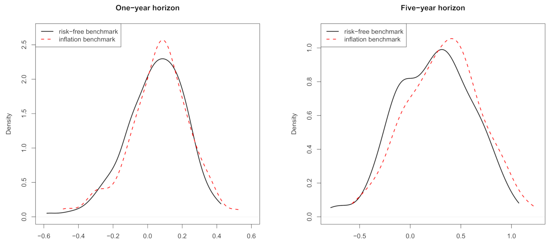
However, the returns transformed with the two benchmarks differ only slightly. A small upward shift under the inflation benchmark is noticeable in Figure 1, which shows density plots of the benchmarked returns for both the one- and five-year horizons.
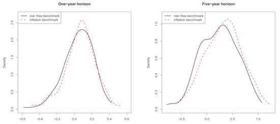
Figure 1.
Kernel density estimates of the probability density function of returns transformed with the risk-free rate benchmark (solid) and the inflation benchmark (dotted). (Left) One-year horizon. (Right) Five-year horizon. Period: 1872–2020. Data: annual S&P 500.
3. Results and Discussion
3.1. One- and Five-Year Excess Stock Return Predictability
In what follows, we apply the double benchmarking approach introduced in Section 2 to the annual U.S. stock market data. The Models (2) and (8) are estimated with a local-linear kernel smoother using the quartic kernel. The optimal bandwidths were chosen by cross-validation, that is, by maximizing the introduced in Equation (10). Note that the linear model is automatically embedded in our approach because of the ability of the local-linear smoother to estimate this simple functional form without any bias. Remember that the value compares the predictive power of a specific model (as a combination of predictive variables) with the predictive power of the historical mean. Thus, the largest positive under each benchmark indicates our favored model with the highest predictive power. We study the empirical findings of values based on different validated scenarios shown for the one- and five-year horizon in Table 3 and Table 4, respectively.

Table 3.
Predictive power (%) for the one-year excess stock returns corresponding to the prediction problem defined in (2). The predictive power is measured by as defined in (10). The benchmarks considered are based on the short-term interest rate () and the inflation rate (). The predictive variables used are , using the indicated benchmark as shown in (4). “–” indicates not applicable cases of matched covariate with benchmark. equals by construction as explained in the footnote in Section 3.1.

For almost all the variable combinations in the one- and five-year cases as well as under both benchmarks, we found a positive , that is, a better predictive power compared with the historical mean. Only the inflation rate as a single covariate under the short-term benchmark has a negative for both horizons and thus no predictive power.
When comparing one- with five-year predictions for the risk-free rate benchmark, we confirmed the findings of Rapach and Zhou [26] that longer-horizon predictions produce more accurate estimates than shorter horizons. All considered combinations of predictive variables have higher values for the five-year case. However, for the inflation benchmark, we observed the contrary, that is, almost all models for the one-year horizon have a higher predictive power. The only exception is the earnings-by-price variable with a slightly increased value in the five-year case.
Under the short interest benchmark , the term spread is the most powerful predictive variable for excess stock returns. In detail, with the prediction constrained to using only single covariates, the term spread is the best predictor for the one- and five-year horizon with and , respectively. Note that and (and their combinations with ) have the same by construction of the transformed spread according to (4). For example, and . Both differ by a constant shift of one, which has no impact on the estimation process with the local-linear smoother. Considering now the models with combined predictive variables, we find in the one-year case that yields , whereas in the five-year case, and perform closely with and , respectively; for both cases, there is thus increased predictive power compared with the best model with the single term spread covariate.
Under the inflation benchmark , the earnings variable is the most powerful single predictor for the one- and five-year horizons with and , respectively. In the one-year case, the pair further boosts the predictive power to , whereas for the five-year horizon, we find the same variable combination to be the most predictive model with .
In our model, which combines both one-year and five-year predictions, we use the optimal combination of predictive variables for each benchmark and horizon. For convenience, Table 5 summarizes the best models. For consistency and to examine the robustness of our results, we additionally consider the second-best set of predictors under the risk-free rate benchmark for the five-year horizon, that is, .

Table 5.
Summarized optimal combinations of predictive variables and their predictive power (%).
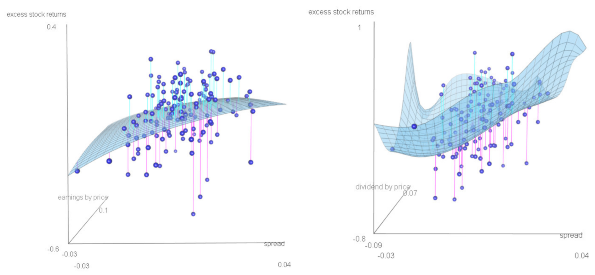
To obtain deeper insights into the relationship between excess stock returns and the predictive variables for the different benchmarks and horizons discussed above, Figure 2 and Figure 3 show the estimated nonparametric function (light blue surface) together with the underlying observations (dark blue balls). Especially for the risk-free rate benchmark, a nonlinear relationship is notable. However, the estimated function seems to be more stable under the inflation benchmark, that is, it is very similar for the one- and five-year horizons. All four plots indicate that with an increase in the spread, the predicted return increases, holding other factors fixed. An increase in the earnings predicts an increase in the return. Note that this effect is stronger for the inflation than for the risk-free rate benchmark. The dividend-by-price versus excess stock return relation for a fixed spread under the risk-free rate benchmark and the five-year horizon is U-shaped.

Figure 2.
Risk-free rate benchmark. The relation between excess stock returns and predictive variables: the earnings-by-price ratio and the spread, one-year horizon (left); the dividend-by-price ratio and the spread, five-year horizon (right). Estimated nonparametric function (light blue surface) and observations (dark blue balls). Period: 1872-2020. Data: annual S&P 500.
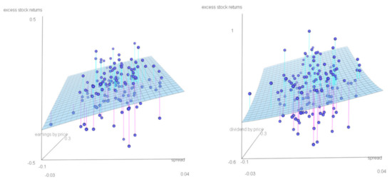
Figure 3.
Inflation benchmark. Relation between excess stock returns and predictive variables: the earnings-by-price ratio and the spread, one-year horizon (left); the earnings-by-price ratio and the spread, five-year horizon (right). Estimated nonparametric function (light blue surface) and observations (dark blue balls). Period: 1872-2020. Data: annual S&P 500.
3.2. Short-Term Exuberance and Long-Term Stability: Combining Predictions of Short and Long Horizons
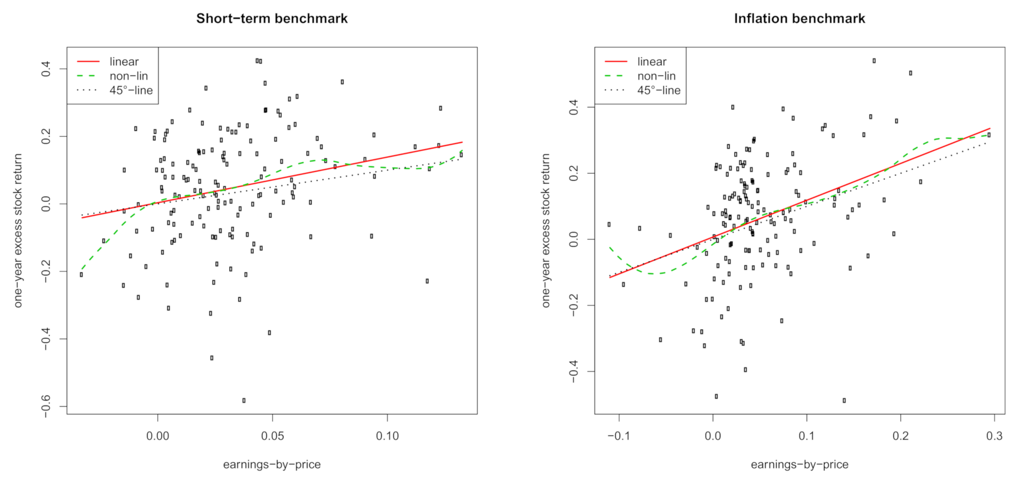
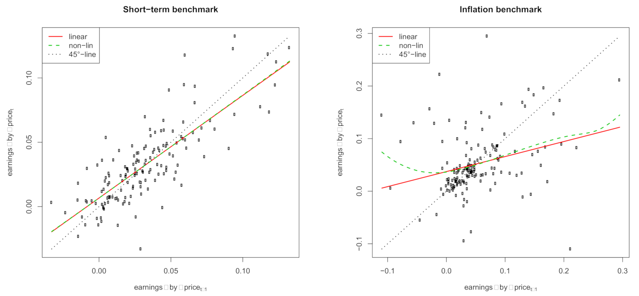
In this section, we illustrate the main empirical contribution of our paper. Recall that the simple econometric model introduced in Section 2.4, which combines short- and long-term predictions, builds on (a) the predictive power of earnings for excess stock returns with its linear model formulation of Equation (12) and (b) the autoregressive development of order one of the earnings in Equation (11). Table 6 shows the estimated OLS coefficients and regression summaries of the linear Models (11) and (12). We find that the earnings variable has more predictive power for excess stock returns under the inflation benchmark than the short-term benchmark: the of the former is more than twice as large as that of the latter ( versus ). The autoregressive behavior of the earnings is stronger in terms of for the short-term benchmark than the inflation benchmark ( versus ). However, the much smaller estimated coefficient under the inflation benchmark ( versus ) indicates a more stable variation in the earnings around the scaled historical mean. The intercept is also significantly differently estimated from zero for both benchmarks. Figure 4 and Figure 5 show the linear Models (11) and (12) for both benchmarks (solid red line) together with estimates of the local-linear smoother (dashed green line) and the -line (dotted black line). These illustrations verify the usefulness of using linear functions in our econometric model in Section 2.4.

Table 6.
Estimated parameters (and standard errors in parentheses) of the linear Models (11) and (12) used for the econometric model in Section 2.4 under the short-term interest rate benchmark or the inflation benchmark. , the standard coefficient of determination of a linear model; Adj. , the adjusted ; Num. obs., the number of observations used in the regression; RMSE, root mean square error.
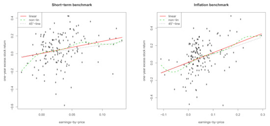
Figure 4.
Relation between excess stock returns and the earnings-by-price ratio. (Left) Short-term interest rate benchmark. (Right) Inflation benchmark. Shown are estimates of a linear function (solid red), the local-linear smoother (dashed green), and the 45-line (dotted black). Period: 1872–2020. Data: annual S&P 500.
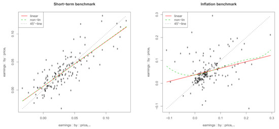
Figure 5.
Autoregressive behavior of the earnings-by-price ratio. (Left) Short-term interest rate benchmark. (Right) Inflation benchmark. Shown are estimates of a linear function (solid red), the local-linear smoother (dashed green), and the 45-line (dotted black). Period: 1872–2020. Data: annual S&P 500.
The next step in running our model is its calibration to the conditional mean and variance estimates for the one- and five-year horizons (the right-hand side values in Equation (23)); Table 7 shows those estimates for both benchmarks. Note that we used out-of-sample predictions from the optimal models discussed in Section 3.1 for both horizons (see also Table 5), that is, and are based on the newest predictive variables in our records (corresponding to December 2019 values). For the short-term benchmark, the optimal models predict returns of (1 year) and (5 years). Note that the average annual return for the five-year horizon of is smaller than the predicted return for the one-year horizon of . The econometric model should be able to adequately capture such a decline in annual returns and we exactly achieved this, as we show later, via the simple linear correction proposed in Section 2.4. For the inflation benchmark, the corresponding predictions are (1 year) and (5 years). Although the picture is similar for the one-year horizon, the behavior of the five-year predictions is different. We forecast an increase in one-year real returns as the average annual return for the five-year horizon of , which is now larger than the predicted return for the one-year horizon of .

Table 7.
Estimated parameters of the econometric model under the short-term interest rate benchmark or the inflation benchmark (in %). For (conditional) predictions of the mean , the variable combination with the largest is used (Table 5). denotes the estimated standard deviation of the predictions or , is the sample standard deviation of or (Table 2). , , , and are the parameter estimates of the econometric model in Section 2.4.
From the upper panel of Table 7, the standard deviations of predicted one-year and five-year returns, and , respectively, appear reduced compared with the standard deviation of observed returns through the statistical modeling process for both benchmarks (Equations (21) and (22)). Under the short-term benchmark, we obtain a reduction from to (1 year) and to (5 years), whereas under the inflation benchmark, from to (1 year) and to (5 years). Note that our model combining the one- and five-year horizons further reduces the uncertainty and thus the risk for one-year returns under both benchmarks, as we explain below.
Using the estimated coefficients of the linear Models (11) and (12) (, , , and ) as well as the predicted one-year and five-year returns and estimated variation (, , , and ), we solve the equation system (23) and obtain the estimates , , , and (Equations (24)–(27)) reported in the lower panel of Table 7 for both benchmarks. For the inflation benchmark, we obtain and , i.e., an intercept in our simple linear correction of predicted one-year returns (13)–(15), which is close to zero and a slope near one. This implies that only a slight correction suffices in combining optimal one-year and five-year stock return predictions. However, under the short-term benchmark, a much stronger correction is necessary to model the decline in the one-year returns over time: and . Table 8 shows the development of the one-year returns for the periods of interest, i.e., from to for both benchmarks. Note that the corrected risk premium equals in period by construction, reduces over time to in period , and sums up over the five-year horizon to again by construction. Similarly, the corrected real return equals in period by construction, increases from year to year to in period , and sums up to the five-year prediction of . The underlying development of the earnings and the simple return predictions from Models (11) and (12) are also shown in Table 8.

Table 8.
Predicted excess stock returns from the econometric model in Section 2.4 under the short-term interest rate benchmark or the inflation rate benchmark. is the last earnings-by-price observation in our records (transformed according to the benchmark A) and corresponds to December 2019. denotes the one-year predictions of excess stock returns from the linear Model (12) (parameter estimates in Table 6) and is their corrected counterparts based on (13)–(15) (parameter estimates in Table 7).
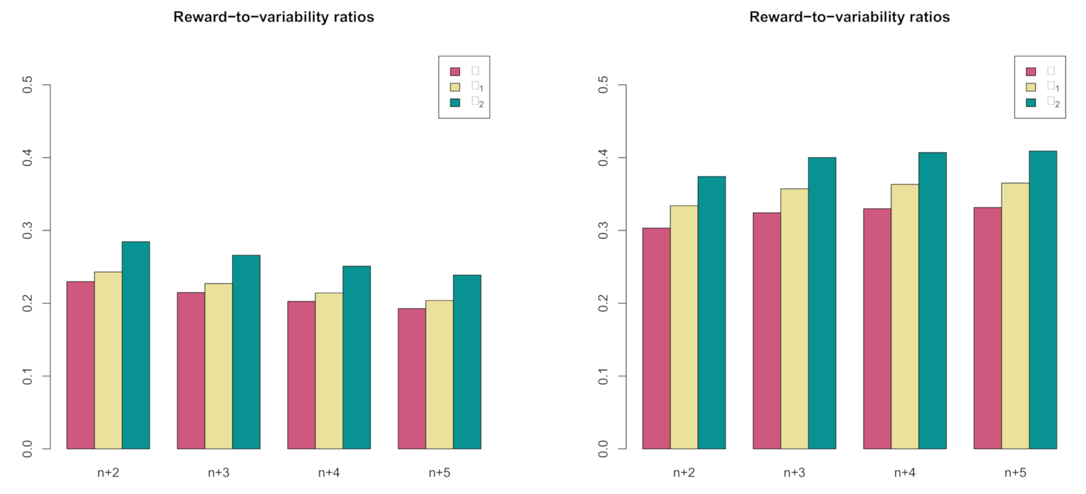
Another important outcome of our econometric model is the additionally reduced variation in the corrected one-year returns of the periods to . For the short-term benchmark, Table 7 reports a reduction from to , that is, a drop in variation of compared with the sample standard deviation of one-year returns of —the starting point of our analysis. Similarly, for the inflation benchmark, reduces to , that is, a decrease in variation of from the sample standard deviation of one-year returns of . tells us that in predicted pure one-year returns (i.e., ignoring the long-term view), a sort of bubble is still present. In other words, even short-term predictions of the one-year horizon are prone to speculative exuberance. However, our simple model optimizes the one-year investments according to the bubble-free long-term variance, reducing the variation/risk. This finding is relevant for long-term investors (above one year), i.e., for the majority of us via our pensions. Figure 6 illustrates this discussion and shows reward-to-variability ratios for each benchmark A based on the corrected one-year predictions for the periods to and the three standard deviations in the model , , and .

Figure 6.
Comparison of reward-to-variability ratios based on corrected one-year predictions for periods and (red), (yellow), and (green). (Left) Short-term interest rate benchmark. (Right) Inflation benchmark.
Finally, we repeat the model calibration for an alternative set of predictors under the risk-free rate benchmark for the five-year case, that is, the combination of earnings and term spread, aiming for congruity in the choice of the baseline set of predictors across benchmarks and horizons. Analagous to the reports in Table 7 and Table 8, Table A1 presents our estimates, which are minimally affected by this choice, whereas Table A2 exhibits the development of the earnings and return predictions, which remain qualitatively similar.
3.3. A Final Comment on the Performance and the Choice of the Benchmark
Notice that our underlying estimates when considering the inflation benchmark are more stable than in the equivalent short-term interest case. The autoregressive earnings model is also more stable in the inflation case compared with the short-term interest case, with a much higher mean-reversion. The modeling of excess returns shows a linear shape in the inflation case (Figure 3) but has considerable variability in the short-term interest case (Figure 2). Adjusting under the inflation benchmark from a one-year model to a five-year model is non-dramatic, contrary to the complete change involved in the short-term interest case. Although both models perform similarly after validation by the short-term interest rate being ahead in the long-term case, we might tend to prefer to work with the stable and intuitive inflation benchmark when providing our long-term and short-term model of stock returns. The choice of the benchmark depends on the ultimate application. If one follows, for example, one of the key messages of Merton [2], then forecast, especially for pensions, should be net of inflation.
4. Concluding Remarks
We propose a state-of-the-art econometric model that accounts contemporaneously for short- and long-term predictions. Therefore, it serves for short-term market timing as well as a long-term asset-allocation strategy for the long-term saver. The combination of the one- and five-year investment horizons thereby reduces the short-term variation by almost 20%. This finding has several implications: First, the high sample standard deviation of short-term returns indicates the presence of bubbles even in one-year returns. Second, institutional long-term investors such as pension funds should disregard pure short-term econometric models when deciding on their long-term asset allocation. Third, for a given risk appetite level, the ability to add equity exposure to result in increased long-term savers’ portfolio return is significant as it provides better pensions for everyone (see also [2,3]). Fourth, we found the inflation benchmark that expresses everything in real terms to be more stable than the often-used short-term interest rate benchmark. The former perfectly links with Merton’s [2] pension vision and provides good predictive power based on our empirical results.
We applied our framework to U.S. stock market excess returns and common predictors based on the short-term interest rate or the inflation benchmark for the one- and five-year horizons. Of potential interest are reference rates [13], longer horizons (say ten years) [27], or econometric modeling of the conditional variance [28], but these tasks remain for future research.
Author Contributions
Conceptualization, I.K., P.M., J.P.N. and M.S.; Formal analysis, I.K., P.M., J.P.N. and M.S.; Funding acquisition, J.P.N.; Investigation, P.M.; Methodology, M.S.; Software, M.S.; Supervision, J.P.N.; Writing—original draft, I.K., P.M., J.P.N. and M.S. All authors contributed equally to this work. All authors have read and agreed to the published version of the manuscript.
Funding
The authors thank the University of Graz for the open access funding.
Institutional Review Board Statement
Not applicable.
Informed Consent Statement
Not applicable.
Data Availability Statement
Financial data was obtained from http://www.econ.yale.edu/~shiller/data.htm (accessed on 16 April 2020) and https://fred.stlouisfed.org/series/TB6MS (accessed on 16 April 2020).
Acknowledgments
The authors thank the Open Access Funding by the University of Graz.
Conflicts of Interest
The authors declare no conflict of interest.
Appendix A
In Section 2.2, we introduce our setup for the T-year predictions. Here, we describe in more detail important single steps. Equation (5) defines as the sum of annual continuously compounded returns, which are of an overlapping nature:
where n is the number of observations of one-year returns. Using the relations stated in Equation (6), we easily obtain
where

Table A1.
Estimated parameters of the econometric model under the short-term interest rate benchmark or the inflation benchmark based on common predictive variables (earnings and spread) for one- and five-year horizons. Changes (compared to Table 7) are provided in boldface. See also the notes in Table 7.
| Benchmark | Short-Term Interest Rate | Inflation Rate | ||||||
|---|---|---|---|---|---|---|---|---|
| One-year () | 4.30 | 16.34 | 10.67 | 17.28 | 4.15 | 16.38 | 17.53 | 18.04 |
| Five-year () | 20.93 | 32.41 | 21.78 | 36.65 | 27.41 | 33.52 | 14.85 | 36.33 |
| Parameter estimate | 6.27 | −0.48 | 16.34 | 14.00 | −0.17 | 0.95 | 16.38 | 14.62 |

Table A2.
Predicted excess stock returns from the econometric model in Section 2.4 under the short-term interest rate benchmark or the inflation rate benchmark based on common predictive variables (earnings and spread). Changes (compared to Table 8) are provided in boldface.
Table A2.
Predicted excess stock returns from the econometric model in Section 2.4 under the short-term interest rate benchmark or the inflation rate benchmark based on common predictive variables (earnings and spread). Changes (compared to Table 8) are provided in boldface.
| Benchmark | Short-Term Interest Rate | Inflation Rate | ||||
|---|---|---|---|---|---|---|
| Period | ||||||
| n | 2.76 | – | – | 3.47 | – | – |
| 2.87 | 4.08 | 4.30 | 4.72 | 4.56 | 4.15 | |
| 2.95 | 4.23 | 4.23 | 5.08 | 5.95 | 5.47 | |
| 3.02 | 4.34 | 4.17 | 5.18 | 6.35 | 5.85 | |
| 3.07 | 4.43 | 4.13 | 5.21 | 6.47 | 5.95 | |
| – | 4.50 | 4.10 | – | 6.50 | 5.98 | |
References
- Lioui, A.; Poncet, P. Long horizon predictability: An asset allocation perspective. Eur. J. Oper. Res. 2019, 278, 961–975. [Google Scholar] [CrossRef]
- Merton, R.C. The crisis in retirement planning. Harv. Bus. Rev. 2014, 92, 43–50. [Google Scholar]
- Gerrard, R.; Hiabu, M.; Kyriakou, I.; Nielsen, J.P. Communication and personal selection of pension saver’s financial risk. Eur. J. Oper. Res. 2019, 274, 1102–1111. [Google Scholar] [CrossRef]
- Gerrard, R.; Hiabu, M.; Nielsen, J.; Vodicčka, P. Long-term real dynamic investment planning. Insur. Math. Econ. 2020, 92, 90–103. [Google Scholar] [CrossRef]
- Carmona, J.; León, A.; Vaello-Sebastià, A. Does stock return predictability affect ESO fair value? Eur. J. Oper. Res. 2012, 223, 188–202. [Google Scholar] [CrossRef]
- Bodnar, T.; Parolya, N.; Schmid, W. On the exact solution of the multi-period portfolio choice problem for an exponential utility under return predictability. Eur. J. Oper. Res. 2015, 246, 528–542. [Google Scholar] [CrossRef]
- Kyriakou, I.; Mousavi, P.; Nielsen, J.P.; Scholz, M. Longer-Term Forecasting of Excess Stock Returns–The Five-Year Case. Mathematics 2020, 8, 927. [Google Scholar] [CrossRef]
- Lettau, M.; Van Nieuwerburgh, S. Reconciling the return predictability evidence. Rev. Financ. Stud. 2008, 21, 1601–1652. [Google Scholar] [CrossRef]
- Chen, Q.; Hong, Y. Predictability of Equity Returns over Diferent Time Horizons: A Nonparametric Approach; Working Paper; Cornell University/Department of Economics: Ithaca, NY, USA, 2009. [Google Scholar]
- Scholz, M.; Nielsen, J.P.; Sperlich, S. Nonparametric prediction of stock returns based on yearly data: The long-term view. Insur. Math. Econ. 2015, 65, 143–155. [Google Scholar] [CrossRef]
- Scholz, M.; Sperlich, S.; Nielsen, J.P. Nonparametric long term prediction of stock returns with generated bond yields. Insur. Math. Econ. 2016, 69, 82–96. [Google Scholar] [CrossRef]
- Cheng, T.; Gao, J.; Linton, O. Nonparametric Predictive Regressions for Stock Return Predictions; Cambridge Working Papers in Economics: 1932; Faculty of Economics, University of Cambridge: Cambridge, UK, 2019. [Google Scholar]
- Kyriakou, I.; Mousavi, P.; Nielsen, J.P.; Scholz, M. Forecasting benchmarks of long-term stock returns via machine learning. Ann. Oper. Res. 2021, 287, 221–240. [Google Scholar] [CrossRef]
- Nielsen, J.P.; Sperlich, S. Prediction of stock returns: A new way to look at it. ASTIN Bull. 2003, 33, 399–417. [Google Scholar] [CrossRef][Green Version]
- Xiao, Z.; Linton, O.B.; Carroll, R.J.; Mammen, E. More efficient local polynomial estimation in nonparametric regression with autocorrelated errors. J. Am. Stat. Assoc. 2003, 98, 980–992. [Google Scholar] [CrossRef]
- Su, L.; Ullah, A. More efficient estimation in nonparametric regression with nonparametric autocorrelated errors. Econom. Theory 2006, 22, 98–126. [Google Scholar] [CrossRef]
- Linton, O.B.; Mammen, E. Nonparametric transformation to white noise. J. Econom. 2008, 142, 241–264. [Google Scholar] [CrossRef]
- Geller, J.; Neumann, M.H. Improved local polynomial estimation in time series regression. J. Nonparametr. Stat. 2018, 30, 1–27. [Google Scholar] [CrossRef]
- De Brabanter, K.; De Brabanter, J.; Suykens, J.; De Moor, B. Kernel regression in the presence of correlated errors. J. Mach. Learn. Res. 2011, 12, 1955–1976. [Google Scholar]
- Bergmeir, C.; Hyndman, R.J.; Koo, B. A note on the validity of cross-validation for evaluating autoregressive time series predictions. Comput. Stat. Data Anal. 2018, 120, 70–83. [Google Scholar] [CrossRef]
- Opsomer, J.; Wang, Y.; Yang, Y. Nonparametric regression with correlated errors. Stat. Sci. 2001, 16, 134–153. [Google Scholar]
- Chu, C.K.; Marron, J.S. Comparison of two bandwidth selectors with dependent errors. Ann. Stat. 1991, 19, 1906–1918. [Google Scholar] [CrossRef]
- Burman, P.; Chow, E.; Nolan, D. A cross-validatory method for dependent data. Biometrika 1994, 81, 351–358. [Google Scholar] [CrossRef]
- Shiller, R.J. Market Volatility; MIT Press: Cambridge, MA, USA, 1989. [Google Scholar]
- Welch, I.; Goyal, A. A comprehensive look at the empirical performance of equity premium prediction. Rev. Financ. Stud. 2008, 21, 1455–1508. [Google Scholar] [CrossRef]
- Rapach, D.; Zhou, G. Forecasting Stock Returns. In Handbook of Economic Forecasting, 2nd ed.; Elliott, G., Timmerman, A., Eds.; Elsevier: Amsterdam, The Netherlands, 2013; pp. 328–383. [Google Scholar]
- Munk, C.; Rangvid, J. New Assumptions of a pension forecast model: Background, level and consequences for individuals forecasted pension. Finans/Invest 2018, 6, 6–14. [Google Scholar]
- Mammen, E.; Nielsen, J.P.; Scholz, M.; Sperlich, S. Conditional Variance Forecasts for Long-Term Stock Returns. Risks 2019, 7, 113. [Google Scholar] [CrossRef]
Publisher’s Note: MDPI stays neutral with regard to jurisdictional claims in published maps and institutional affiliations. |
© 2021 by the authors. Licensee MDPI, Basel, Switzerland. This article is an open access article distributed under the terms and conditions of the Creative Commons Attribution (CC BY) license (http://creativecommons.org/licenses/by/4.0/).

