Gaussian Pseudorandom Number Generator Using Linear Feedback Shift Registers in Extended Fields

Abstract

A new proposal to generate pseudorandom numbers with Gaussian distribution is presented. The generator is a generalization to the extended field $GF\left(2^n\right)$ of the one using cyclic rotations of linear feedback shift registers (LFSRs) originally defined in $GF\left(2\right)$. The rotations applied to LFSRs in the binary case are no longer needed in the extended field due to the implicit rotations found in the binary equivalent model of LFSRs in $GF\left(2^n\right)$. The new proposal is aligned with the current trend in cryptography of using extended fields as a way to speed up the bitrate of the pseudorandom generators. This proposal allows the use of LFSRs in cryptography to be taken further, from the generation of the classical uniformly distributed sequences to other areas, such as quantum key distribution schemes, in which sequences with Gaussian distribution are needed. The paper contains the statistical analysis of the numbers produced and a comparison with other Gaussian generators.

1. Introduction

Random number generators are of vital importance in many areas and, particularly, in cryptography. Most cryptographic algorithms and protocols make use of random or pseudorandom numbers. Encryption and authentication schemes in wireless and mobile communications, such as Bluetooth [1], IEEE 802.15.4, IEEE 802.11 WLAN [2], GSM [3] or LTE [4], employ pseudorandom numbers; radio frequency identification [5] standards define and recommend the utilization of true random numbers [6].A large part of the pseudo-random number generators (PRNGs) used in cryptography are based on linear feedback shift registers (LFSRs), mainly due to their simplicity, low cost of implementation, good statistical behavior and the possibility of using a mathematical model that allows the generator to be designed for an optimal performance [7].

In fact, the maximal sequence length generated by an LFSR of m cells is $2^m-1$. However, those sequences suffer from a high predictability in such a way that the whole sequence can be reproduced if an eavesdropper gains access to $2m$ bits. Despite that, the LFSR is still an important part of the cryptographic generators because those sequences are used to derive more robust ones but keeping the original statistical properties. Two main methods are applied to fix that weakness: nonlinear combination and nonlinear filtering. The former is based on several LFSR, usually with different number of cells [3], and the latter on a unique LFSR whose sequence is processed (filtered) by a nonlinear function [4].

Another advantage of using LFSRs in cryptography is that the sequences generated have a uniform statistical distribution. For all these reasons, there is a lot of published works related to the LFSR, but only a few regarding its utilization to produce numbers with Gaussian distribution.

More precisely, in 2010, Kang [8] proposed a Gaussian PRNG, using a LFSR of length $N=4M$ bits, to generate pseudorandom numbers of $(M+4)$ bits. The numbers were produced by means of an accumulator applied on decimated M-bits numbers, producing a sequence of length $(2^N-1)/\left(8N\right)$. In order to fix this LFSR oversizing, Condo et al [9] proposed, in 2015, a Gaussian PRNG using permutations over the successive states of a unique LFSR, thus reducing the implementation cost. The main drawback is that not all the possible permutations yield numbers with the required Gaussian distribution and, consequently, a high computational effort must be performed to find the suitable permutations. Later, in 2020, Cotrina et al [10] presented an improvement of the Condo’s PRNG focusing on a particular type of permutations of the LFSR state, the cyclic rotations. The authors concluded that more than $90\%$ of the cycle rotations are usable for the PRNG and produce Gaussian distributed numbers.

These proposals are based on the central limit theorem (CLT) [11], trying to obtain a Gaussian distribution using sequences of uniformly distributed numbers. In this sense, the first proposal [12] employed several LFSRs to generate independent sequences of numbers. However, most of the proposals use a unique LFSR to generate all the sequences, such as those of Kang [8], Condo [9] and Cotrina [10].

Following the same approach, the present paper describes a Gaussian PRNG based on an LFSR operated and defined in an extension field $GF\left(2^n\right)$ instead of using the binary field $GF\left(2\right)$. An LFSR in $GF\left(2^n\right)$ can be represented as a combination of n LFSR in $GF\left(2^n\right)$. This fact, as it is described later, allows a particular implementation of the CLT. Furthermore, as it can be deduced from the equivalent model, the cyclic rotations proposed by Cotrina [10], as a particular case of the permutations proposed by Condo [9], are implicitly included in the operations of an LFSR in $GF\left(2^n\right)$. This proposal is also in line with the trend of using cryptographic algorithm and protocols in extended fields to take advantage of the word length of processors [13].

On the other hand, the proposed generator is a way to keep using the LFSR as a basic element to generate pseudorandom numbers in cryptographic areas where other than uniform distribution is required. An example of this is quantum key distribution (QKD) schemes [14]. This type of scheme, designed to establish keys between two endpoints, can be considered the most mature application of quantum communications. Currently, all developed countries have deployed QKD schemes, some experimentally (in controlled environments) and others in their current transit networks [15]. The first QKD schemes were based on the transmission of polarized photons using non-orthogonal states. These schemes, named discrete-variable QKD (DV-QKD) [16,17], require the utilization of specific components for single-photon detection. A different type of QKD scheme has been developed to carry information on some continuous properties of the light, such as the values of the quadrature components of a coherent state. The so-called continuous-variable QKD (CV-QKD) [18,19,20,21], currently deployed in several countries e.g., China, Japan, Spain and Italy [15] present a lower implementation cost due to the utilization of standard communications components. They use coherent detection techniques usually employed in classical optical communications. Furthermore, they employ Gaussian modulation to send random amplitude and phase values that must be generated following a Gaussian distribution [10,14,22].

Section 2 introduces the fundamentals of the LFSR in the binary and extended Galois fields. Section 3 describes the binary equivalent model of an LFSR defined in a $GF\left(2^n\right)$ and the proposal of a Gaussian PRNG based on this model. The statistical analysis of the numbers produced by the proposed PRNG is presented in Section 4 and compared to the Box–Muller [23,24] algorithm, a well-known algorithm not based on CLT. Finally, conclusions are presented in Section 5.

2. LFSR Fundamentals

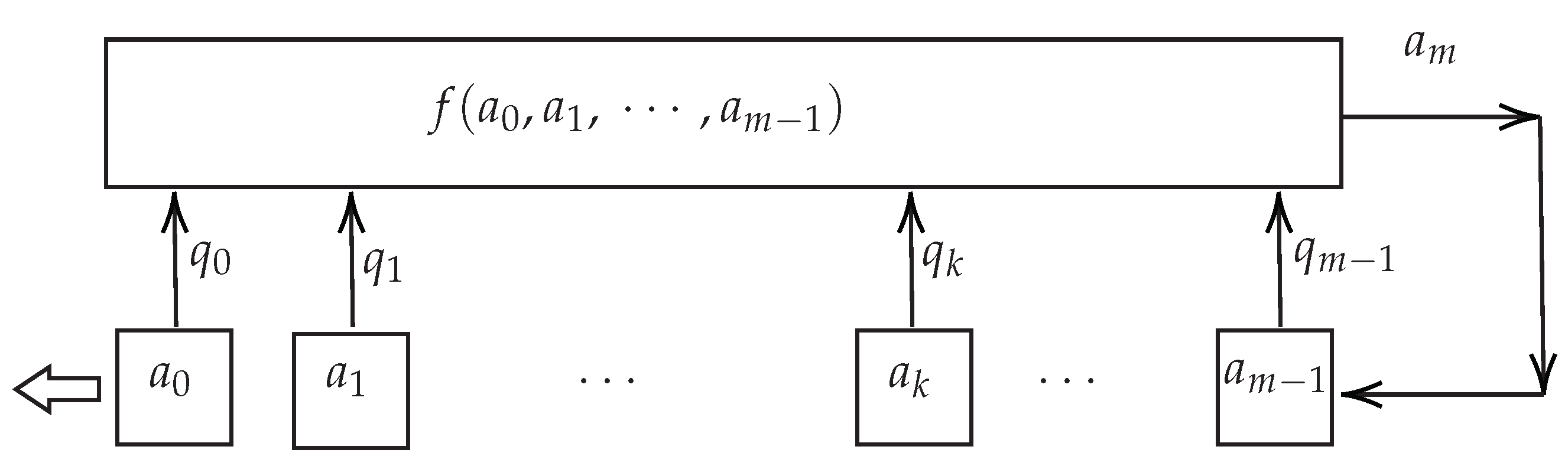
In this section the basic properties of the linear feedback shift register (LFSR) (see Figure 1), and its generated sequences are described.

A linear feedback shift register (LSFR) is a shift register that takes a linear function of a previous state as an input. Most commonly. The LFSR [25] of length m consists of m stages numbered $0,1,2,\cdots m-1$, each capable of storing one bit and having one input and one output and a clock which controls the movement of data.

Definition 1.

An LFSR of length m consists of: A linear feedback shift register (LFSR) of length m consists of m stages numbered $0,1,2,\cdots m-1$, each capable of storing one bit and having one input and one output; and a clock which controls the movement of data. During each unit of time the following operations are performed:

• The content of stage 0 is output and forms part of the output sequence.
• The content of stage i is moved to stage $i-1$ for each i where $1\le i\le m-1$.
• The new content content of state $m-1$ is the feedback bit $a_j$ which is calculated by adding together modulo 2 the previous contents of a fixed subset of stages $0,1,\cdots ,m-1$.

The values $q_i$ are either 0 or 1 and the feedback bit $a_j$ is the modulo 2 sum of the contents of those stages i, $1\le i\le m-1$, for which $q_{m-i}=1$. As a consequence, the output sequence of the LFSR is $A=\left(a_0,a_1,a_2,\cdots \right)$ and is uniquely determined by the following recursion:

$$a_j=f(a_{j-m},a_{j-m+1},\cdots ,a_{j-1})=q_0·a_{j-m}+q_1·a_{j-m+1}+\cdots +q_m·a_{j-1}$$

(1)

The evolution of the LFSR and their sequences generated can be performed by means of a polynomial whose coefficients are the values $q_i$ that represents the stages used to compute the feedback bit $a_j$. For this reason, the LFSR is denoted $\langle m,p\left(x\right)\rangle$, where $p\left(x\right)=1+q_{1}x+q_2{x}^2+\cdots +q_m{x}^m$ is the connection polynomial.

The LFSR is said to be nonsingular if the degree of $p\left(x\right)$ is m (that is, $q_m=1$). If the initial content of stage i is $a_i\in \{0,1\}$ for each i, $0\le i\le ,m-1$, then $\left[a_{m-1},\cdots ,a_1,a_0\right]$ is called the initial state or seed of the LFSR.

On the other hand, the state of the LFSR at the time t is denoted as

$$s^{\left(t\right)}=\left[a_{m-1+t},\cdots ,a_{t+1},a_t\right]$$

(2)

which corresponds to the application of the recursion in the Equation (1) t consecutive times starting with the seed $s^{\left(0\right)}=\left[a_{m-1},\dots ,a_1,a_0\right]$

Example 1.

Consider the LFSR $\langle 4,1+x+x^4\rangle$. If the initial state of the LFSR is $s^{\left(0\right)}=\left[0,0,0,0\right]$, the output sequence is the zero sequence $A=\left(0,0,\cdots \right)$. For the initial state $s^{\left(0\right)}=\left[0,1,1,0\right]$, the sequence has a length of 15 The following table shows the successive states $s^{\left(t\right)}$. Note that the right-most bit of each state constitutes the output sequence $A=\left(0,1,1,0,0,1,0,0,0,1,1,1,1,0,1,0,\cdots \right)$ as we can see in

Table 1. Values of the Linear Feedback Shift Register (LFSR) $\langle 4,1+x+x^4\rangle$ whose initial state is $\left[0,1,1,0\right]$.

t	${\mathit{s}}^{\left(\mathit{t}\right)}$				t	${\mathit{s}}^{\left(\mathit{t}\right)}$
0	0	1	1	0	8	1	1	1	0
1	0	0	1	1	9	1	1	1	1
2	1	0	0	1	10	0	1	1	1
3	0	1	0	0	11	1	0	1	1
4	0	0	1	0	12	0	1	0	1
5	0	0	0	1	13	1	0	1	0
6	1	0	0	0	14	1	1	0	1
7	1	1	0	0	15	0	1	1	0

.

Definition 2

(cf. [25]). An output sequence A $= \left(a_0,a_1,\cdots \right)$ generated by an LFSR $\langle m,p\left(x\right)\rangle$, is said to be periodic if there exits $j_0\in \mathbb{N}$ such that $a_i=a_{i+j_0}$$\forall i\in \mathbb{N}$. Such $j_0$ is called period of the sequence.

From this definition, the sequence of the example is a periodic sequence with period $L=15$.

One of the advantages of LFSR is the mathematical model that allows one to predict the length of the sequences generated. The following definition and theorem states how and when the maximal length is reached by the sequences.

Definition 3

(cf. [25]). If $p\left(x\right)\in {\mathbb{Z}}_2\left[x\right]$ is a connection polynomial of degree m, then $\langle m,p\left(x\right)\rangle$ is called a maximum length LFSR if the output sequence, with non-zero initial state, has period $2^m-1$. This sequence is called m-sequence.

Definition 4.

A polynomial $p\left(x\right)$ in $GF\left(2\right)\left[x\right]$ is irreducible if it cannot be factored into a product of lower-degree polynomials in $GF\left(2\right)\left[x\right]$. An irreducible polynomial $p\left(x\right)\in GF\left(2\right)\left[x\right]$ of degree $m\in \mathbb{N}$ is said to be primitive if $mi{n}_{n\in \mathbb{N}}\left\{n:p\left(x\right)\mid \left(x-1\right)\right\}=2^m-1$.

Theorem 1

(cf. [7]). An output sequence A generated by an LFSR $\langle m,p\left(x\right)\rangle$ is an m-sequence if and only if the connection polynomial $p\left(x\right)$ is a primitive polynomial. The sequence length is independent of the initial state.

Consequently, a primitive polynomial of degree m will generate a sequence of length $2^m-1$ and the LFSR will run through $2^{m-1}$ different nonzero states, that is, all possible nonzero states. Hence, if we consider each state as an m-bit pseudorandom number, we can say that LFSR produce numbers with uniform distribution.

Besides its maximal length, the m-sequences have many desirable statistical properties that can be summarized in the three Golomb’s postulates [7]. Given a periodic binary sequence $A={\left(a_i\right)}_{i\in \mathbb{N}}$ with period length $L=2^m-1$, it is said to be pseudoradom if the following postulates hold.

• Balance property. In every period, the number of zeros is nearly equal to the number of ones (the disparity does not exceed 1, or $\mid {\sum }_{i=0}^{m-1}{\left(-1\right)}^{a_i}\mid \le 1$.
• In every period, half of the run have length 1, one fourth have length 2, one eighth have length 3, and so on. For each of these lengths there are the same number of runs of 0’s and runs of 1’s.
• Two level autocorrelation. The autocorrelation function $c\left(\tau \right)$ is two-valued given by

  $$c\left(\tau \right)=\left\{\begin{array}{ccc}m\hfill & \mathrm{if}& \tau =0\mathrm{mod}m\\ k\hfill & \mathrm{if}& \tau \ne 0\mathrm{mod}m\end{array}\right.$$

  (3)

  where k is a constant. If $k=-1$ for m odd, or $k=0$ for m even, we say that the sequence has the ideal two level autocorrelation function.
• The ideal $k–$tuple distribution. In every period of A, if each nonzero $k-$tuple $\left(a_1,a_2,a_3,\cdots ,a_k\right)$ occurs q times and the zero $k-$tuple occurs $q^{n-k}-1$ times, then we say that the sequence satisfies the ideal k-tuple distribution.

LFSR over $GF\left(2^n\right)$

Definition 5.

Let’s suppose $(F,+,*)$ be a field with operations + and *, we will say that this field F is a Galois field if the cardinal of field F is finite. If the cardinal of the finite field F is p, then F will be represented as $GF\left(p\right)$.

It is possible to extend the prime field $GF\left(p\right)$ to a field of $p^m$ elements, represented by $GF\left(p^m\right)$, which is called an extension field of $GF\left(p\right)$. In our case we shall work for $p=2$.

To build up the field extension of $GF\left(2\right)$, $GF\left(2^n\right)$, let’s consider $p\left(x\right)$ a primitive polynomial over $GF\left(2\right)$ of degree n, once this polynomial is defined, let’s consider a root $alpha$ of this primitive polynomial, therefore $p\left(\alpha \right)=0$. Let’s consider $GF\left(2^n\right)=\left\{0,1,\alpha ,{\alpha }^2,\cdots ,{\alpha }^{2^n-1}\right\}$. It can be proven that all the elements of $GF\left(2^n\right)$ can be represented by $2^n-1$ distinct non-zero polynomials of $\alpha$ over $GF\left(2\right)$ with degree $m-1$ or less. The $0\in GF\left(2^n\right)$ can be represented as the zero polynomial. Then the set $GF\left(2^n\right)$ with the usual operations is a Galois field with $2^n$ elements.

Example 2.

Let’s build the finite field $GF\left(2^4\right)$ generated by the primitive polynomial $p\left(x\right)=1+x+x^4$. First of all, we consider α to be a root of the primitive polynomial $p\left(x\right)$, then we determine all multiplicative powers of α, ${\alpha }^0=1,{\alpha }^1,\cdots$ until we obtain the multiplicative identity 1 on this field. For any Galois field we will have three representations as shown in

Table 2. Representation of the Galois Field $GF\left(2^4\right)$ over $GF\left(2\right)$ with primitive polynomial $p\left(x\right)=1+x+x^4$ over $GF\left(2\right)$.

Power Representation	Polynomial Representation	Vector Representation
0	0	$\left(0,0,0,0\right)$
1	1	$\left(1,0,0,0\right)$
$\alpha$	$\alpha$	$\left(0,1,0,0\right)$
${\alpha }^2$	${\alpha }^2$	$\left(0,0,1,0\right)$
${\alpha }^3$	${\alpha }^3$	$\left(0,0,0,1\right)$
${\alpha }^4$	$1+\alpha$	$\left(1,1,0,0\right)$
${\alpha }^5$	$\alpha +{\alpha }^2$	$\left(0,1,1,0\right)$
${\alpha }^6$	${\alpha }^2+{\alpha }^3$	$\left(0,0,1,1\right)$
${\alpha }^7$	$1+\alpha +{\alpha }^3$	$\left(1,1,0,1\right)$
${\alpha }^8$	$1+{\alpha }^2$	$\left(1,0,1,0\right)$
${\alpha }^9$	$\alpha +{\alpha }^3$	$\left(0,1,0,1\right)$
${\alpha }^{10}$	$1+\alpha +{\alpha }^2$	$\left(1,1,1,0\right)$
${\alpha }^{11}$	$\alpha +{\alpha }^2+{\alpha }^3$	$\left(0,1,1,1\right)$
${\alpha }^{12}$	$1+\alpha +{\alpha }^2+{\alpha }^3$	$\left(1,1,1,1\right)$
${\alpha }^{13}$	$1+{\alpha }^2+{\alpha }^3$	$\left(1,0,1,1\right)$
${\alpha }^{14}$	$1+{\alpha }^3$	$\left(1,0,0,1\right)$

.

This Table 2 shows how all the elements of the extended Field are obtained. The equivalence has been obtained using the vector notation as a function of one of the roots of the primitive polynomial that generates the extended field. In the same way, it can be observed that the body is generated cyclically and that no equal values are obtained except when it has been cycled and all its elements have been obtained periodically.

According to the Example 2, form this point on, we shall represent the elements of the extended fields using the vector notation, where for example the element $1+{\alpha }^2+{\alpha }^3$ will be represented as $\left(1,0,1,1\right)$.

To generate an LFSR on a $GF\left(2^n\right)$ we will start by determining a primitive polynomial p over $GF\left(2\right)$ that will be used to generate the extended field. Once this polynomial and this field have been set, we choose a primitive polynomial g over $GF\left(2^n\right)$ and a seed or non-zero initial state value ${\beta }_0$ on which the primitive polynomial g is applied. In this way, a value ${\beta }_1$, is obtained by $g\left({\beta }_1\right)$ on which the primitive polynomial g will be applied and thus the process will be repeated.

Example 3.

We consider the $GF\left(2^6\right)$ that has been built using the primitive polynomial $q\left(x\right)=1+x+x^6$. Let’s consider the primitive polynomial $p\left(x\right)$ over $GF\left(2^6\right)$ whose vector representation is $p\left(x\right)=\left\{\left\{1,0,1,1,0,1\right\},\left\{1,0,0,1,0,1\right\},\left\{1,1,0,0,0,1\right\},\left\{1,1,0,1,1,0\right\},\left\{1,0,0,1,0,1\right\}\right\}$. The initial seed will be

$$\left\{\left\{1,0,1,1,0,1\right\},\left\{1,0,0,1,0,1\right\},\left\{1,1,0,0,0,1\right\},\left\{1,1,0,1,1,0\right\},\left\{1,0,0,1,0,1\right\}\right\}$$

(4)

and taking into consideration these conditions the output sequence will be

$$A=\left(\left\{1,0,1,1,1,0\right\},\left\{0,1,0,1,0,1\right\},\left\{1,0,1,1,1,0\right\},\left\{0,1,1,0,0,0\right\},\cdots \right)$$

(5)

As in $GF\left(2\right)$, the LFSR in $GF\left(2^n\right)$ produces an m-sequence if and only of the connection polynomial is primitive. The $m-$ sequence has a period of $2^{m·n}-1$ that corresponds to all nonzero states, where m is the degree of the connection polynomial.

3. Gaussian Number Generator over $\mathit{GF} \left(2^{\mathit{n}}\right)$

To apply the CLT, Gaussian generators based on a single LFSR [8,9,10] try to obtain different sequences of pseudo-random numbers with uniform distribution from the same sequence generated by the LFSR. To do this, they apply permutations—generic in some cases, rotations in others—on each state of the LFSR. In this way, with each number generated by the LFSR, other numbers are also being generated (as many as permutations are applied) and therefore different uniform sequences suitable to be combined in a sequence of numbers are being simultaneously constructed. LFSRs defined on an extended field can be analyzed as the combination of a series of binary LFSRs. For this reason, each state of an LFSR in an extended field is related to the states of a series of binary LFSRs. This relation is the one used to propose a PRNG with Gaussian distribution. Next, the equivalent model of an LFSR defined in an extended field that allows the definition of a Gaussian PRNG with excellent performance is described.

3.1. Binary Equivalent Model of an LFSR in $GF\left(2^n\right)$

As it is known [26], there is a relationship between the $m-$sequences generated in $GF\left(2^n\right)$ and those generated in $GF\left(2\right)$, in such a way that the former can be obtained from the latter. The relationship is established from the feedback polynomials that define each LFSR. Specifically, if $q\left(x\right)$ is the primitive polynomial of degree m that defines the LFSR in $GF\left(2^n\right)$ and therefore generates an $m-$sequence in $GF\left(2^n\right)$, the decimated sequences obtained by taking the $j-$th bit of each element in the $m-$sequence are generated by a binary LFSR with primitive feedback polynomial $h\left(x\right)$ of degree $m·n$, where $h\left(x\right)$ divides $q\left(x\right)$. 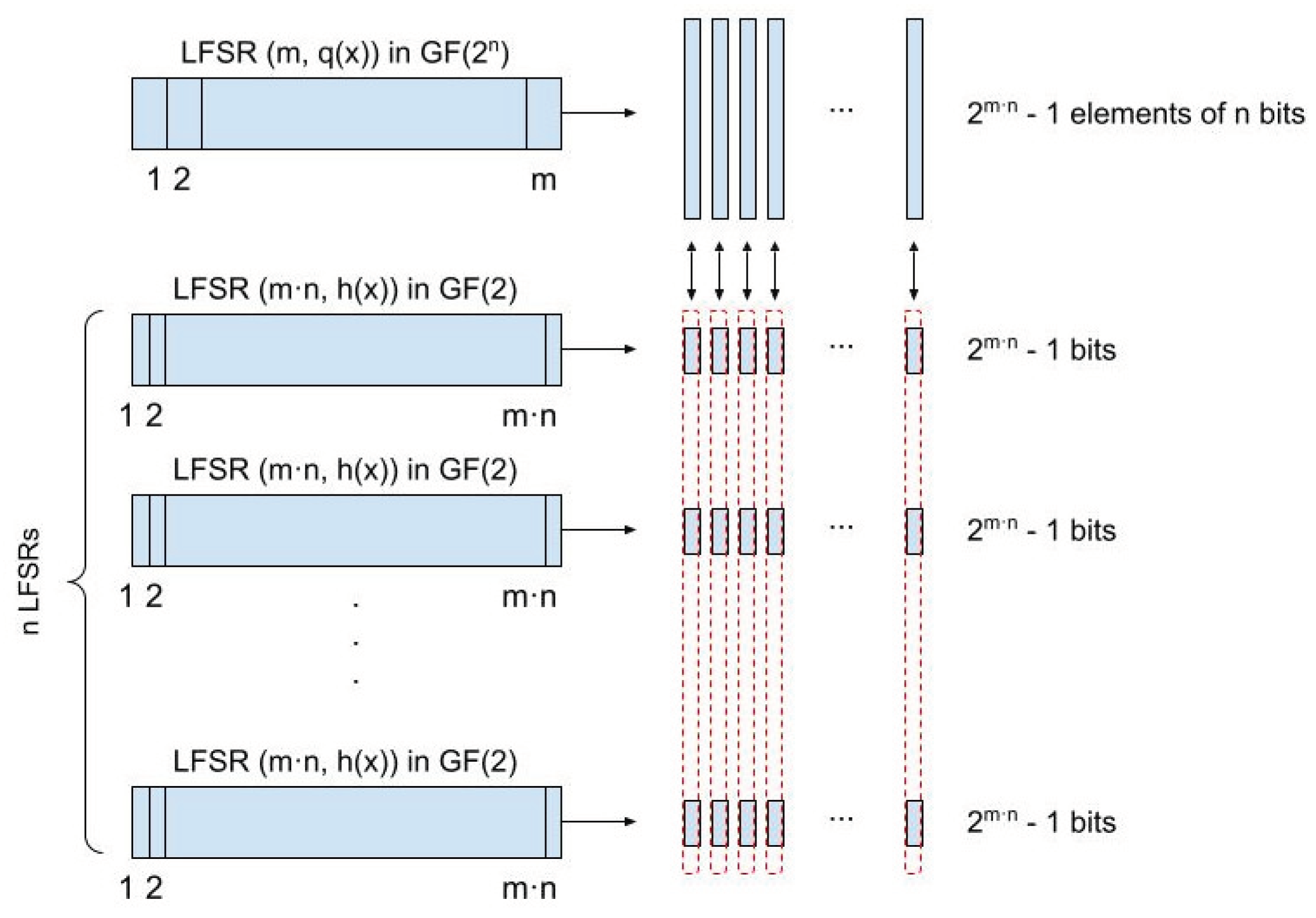This allows to develop an equivalent model of the LFSR defined in $GF\left(2^n\right)$ using n LFSRs in $GF\left(2\right)$, as shown in Figure 2 where the $j-$th bit of each element is generated by the $j-$th binary LFSR. Note that all the binary LFSRs used in the model have the same polynomial $h\left(x\right)$ although initialized in different seeds. Therefore, the sequences generated by the binary LFSRs are $m-$sequences in $GF\left(2\right)$, and consequently, shifted versions of the same sequence. In this way, the generation of an $m-$sequence in $GF\left(2^n\right)$ implies the generation of n binary $m-$ sequences, one for each bit, which can be used as sources with a uniform distribution to later apply CLT.

Definition 6.

Let $〈m,q\left(x\right)〉$ be a LFSR over $GF\left(2^n\right)$. Let $s\left(t\right)=\left[a_{m-1+t},a_{m-2+t},\cdots ,a_t\right]$ be the state of the LFSR at time t, with $a_i\in GF\left(2^n\right)$ that can be represented as the vector $\left[a_{i,n-1},\dots ,a_{i,1},a_{i,0}\right]$ with $a_{i,j}\in GF\left(2\right)$∀$0\le j\le n-1$. Then, ${\mathsf{\Pi }}_k$ is defined as the projection over the $k-$th component of an element. Hence, ${\mathsf{\Pi }}_k\left(a_i\right)=a_{i,k}$ and ${\mathsf{\Pi }}_k\left(s\left(t\right)\right)=s{\left(t\right)}_k=\left[a_{m-1+t,k},a_{m-2+t,k},\cdots ,a_{t,k}\right]$.

This definition allows us to represent the decimated sequences ${\mathsf{\Pi }}_k\left(A\right)$ of a sequence $A=(a_0,a_1,a_2,\cdots )$ as:

$${\mathsf{\Pi }}_k\left(A\right)=({\Pi }_k\left(a_0\right),{\Pi }_k\left(a_1\right),{\Pi }_k\left(a_2\right),\cdots )$$

(6)

Theorem 2.

Let $〈m,q\left(x\right)〉$ be an LFSR over $GF\left(2^n\right)$ and let $〈r_k,f_k\left(x\right)〉$ be the set of all its decimated sequences $\forall k\in \left\{1,2,\cdots ,n\right\}$ then, $q\left(x\right)$ is primitive over $GF\left(2^n\right)$ if and only if $\forall k\in \left\{1,2,\cdots ,n\right\}$$f_k$ is primitive over $GF\left(2\right)$. If these conditions hold, $f_j\left(x\right)=f_k\left(x\right)=h\left(x\right)$$\forall j,k\in \left\{1,2,\cdots ,n\right\}$ and $m\mid r_k$.

Therefore, if we have an LFSR $〈m,q\left(x\right)〉$ over $GF\left(2^n\right)$ where $q\left(x\right)$ is primitive, then we can consider that we have n’s $m-$sequences over $GF\left(2\right)$.

In other words, this equivalent model represents the interleaving process that generates the sequence in $GF\left(2^n\right)$; that is, the sequence generated by the LFSR in $GF\left(2^n\right)$ can be expressed as an interleaved sequence, in the sense describe by Gong in [27], composed by n component sequences, corresponding with the decimated sequences. More precisely, it is a primitive interleaved sequence as all the component sequences are generated by the same primitive polynomial in $GF\left(2\right)$.

On the other hand, pseudorandom sequences must be difficult to reproduce. Linear complexity (or linear span) of a sequence is defined as the degree of the minimal polynomial that generates it, or equivalently the length of the shortest LFSR that generates it. Consequently, the linear complexity of a sequence generated by a primitive LFSR is the length of that LFSR. Hence, considering the sequence produced by an LFSR of m cells in $GF\left(2^n\right)$ as an interleaved sequence, its linear complexity $L{C}_{ext}$ is n times the linear complexity $L{C}_{bin}$ of its primitive components; that is,

$$L{C}_{ext}=n·L{C}_{bin}=m·n^2$$

(7)

3.2. The Proposed Generator

Taking in mind that one of the potential applications of a Gaussian PRNG based in LFSR could be a QKD scheme, it is important to note the following requirements:

• The PRNG should allow a discrete set of values to be generated large enough to approximate the continuous probability distribution.
• The set of values generated must have a Gaussian probability distribution.
• The security of the system must allow the generation of a set of values with a sufficiently large cardinal.
• The generation of obtained values should be done as fast as possible and within the lowest implementation cost. In addition, for the system to be effective, the possibility of a hardware implementation must be considered.
• The system must allow the generation of the pseudo-random values with Gaussian distribution to be different for each of its different executions.

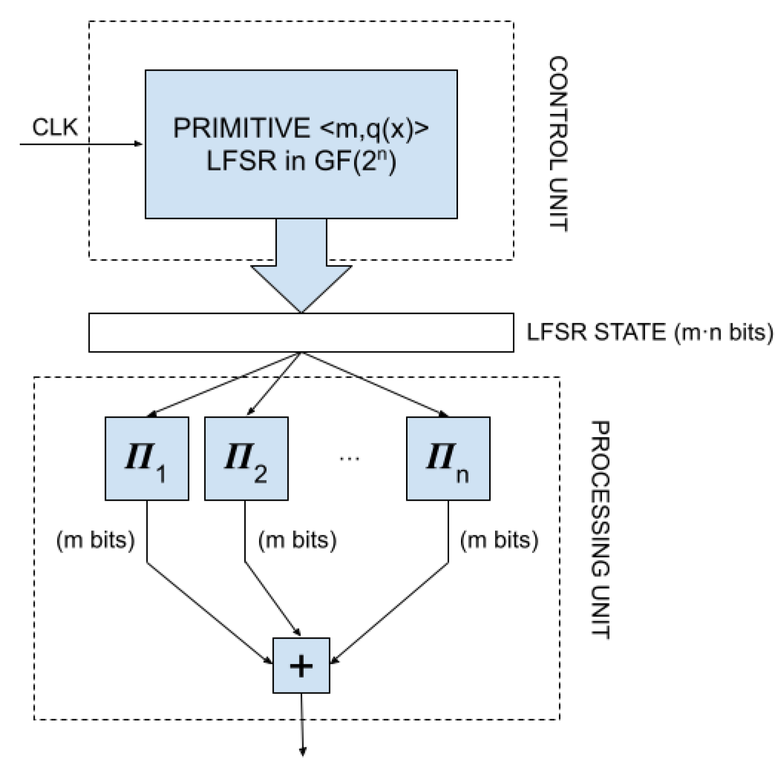
In order to fulfil all the requirements, we propose a PRNG based on an LFSR in $GF\left(2^n\right)$. The PRNG is composed by two units: the control unit and the processing unit (see Figure 3).The control unit consists in an LFSR with m cells, defined by a primitive polynomial $q\left(x\right)$ over $GF\left(2^n\right)$. This unit is responsible for the generation of the basic $m-$sequence from which all the sequences with uniform distribution are obtained for the subsequent application of CLT. As it is described in the previous sections, $ifq\left(x\right)$ is primitive the LFSR generates an $m-$sequence, i.e., a sequence of maximal period $2^{n·m}-1$.

The processing unit has been design with a two-fold objective. On the one hand, like many other cryptosystems, it applies a nonlinear filtering to the sequence produced by the LFSR in the control unit to increase the difficulty that an eavesdropper reproduces the whole sequence. On the other hand, this unit implements the operations that transform the statistical distribution from uniform to Gaussian, i.e., implements the CLT. To do that, the operator ${\mathsf{\Pi }}_k$ is applied on each LFSR state, thus producing n strings of m bits that corresponds with segments of the n binary sequences in the equivalent model described in Section 3.1. Hence, applying the CLT, the pseudorandom number B is obtained by means of the integer sum of those n bitstrings as:

$$B=D\left(s_1^t\right)+D\left(s_2^t\right)+\cdots +D\left(s_n^t\right)$$

(8)

where D is the function that maps an $m-$bit vector $x=(x_0,x_1,\cdots ,x_{n-1})$ into a decimal value,

$$D\left(x\right)=\sum _{i=1}^{n-1}{2}^i·x_i$$

(9)

The period, range and accuracy of the proposed PRNG can be configured using two main parameters: m and n. The sequence of pseudorandom numbers has a period of $2^{mn}-1$ because the feedback polynomial in the LFSR is a degree m primitive polynomial in $GF\left(2^n\right)$. The range of the numbers is mainly determined by m since each state of the LFSR contains $n·m$ bits that split in n strings of m bits later summed to produce the pseudorandom number. The parameter n increases slightly, until $m+lo{g}_2\left(n\right)$, the number of bits of the generated numbers due to the carry of the integer sum. Thus, for $m=5$ and $n=8$, the PRNG generates values with a range of $5+3=8$ bits.

Finally, when the CLT is applied to obtain a Gaussian distribution, its accuracy is related to the numbers of uniform distributed numbers that are summed. In this case, each pseudorandom number is obtained summing n values. Hence, generating $16-$bit pseudorandom numbers requires the utilization of an LFSR with 16 cells. If the LFSR operates in $GF\left(2^4\right)$, the PRNG will present a period of $2^{4·16}-1=2^{64}-1$, obtained from the addition of 4 uniformly distributed sequences. The accuracy may increase using 8 values instead of 4. In that case, the LFSR would work in $GF\left(2^8\right)$ what would also increase the period to $2^{16·8}-1=2^{128}-1$.

Regarding the speed of generation, although, generally, the use of LFSRs in $GF\left(2^n\right)$ is motivated by the speed increase that is achieved by generating n bits instead of 1 in each iteration, in this case, the use of the LFSR in $GF\left(2^n\right)$ pursues a second objective: to take advantage of the implicit relationship with n different binary sequences. This makes it easy to apply the CLT by using a single LFSR that is equivalent to n binary LFSRs. Therefore, the final rate of generating numbers with Gaussian distribution is the same as the rate at which a binary LFSR generates a bit. However, taking into account that the generated numbers are m bits long, the generation speed in bits per second is m times higher.

4. Statistical Analysis

In this section, the distribution of the numbers generated by the proposed PRNG is analyzed. Several normality tests have been applied to identify the configurations that generates numbers with Gaussian distribution.

4.1. Distribution Fit Test

Goodness-of-fit tests are used to evaluate how well a proposed model fits or predicts a particular data set. Usually, test statistics compute deviations between the observed data and predictions from the model. The value of a test statistic is said to be statistically significant if it is found to be within the rejection area of the distribution of the test statistic under the assumption that the model is true. The rejection area is often the upper its significance level $\alpha$ of $5\%$ or $10\%$ of the distribution frequencies. In our work we have set this acceptance minimum level to $10\%$. Therefore a distribution fit test performs a goodness of fit hypothesis test with null hypothesis $H_0$ that data was drawn from a population with a specific distribution of values, in this case the Normal distribution, and alternative hypothesis that it was not.

Usually, a statistical hypothesis test returns a value called p or the p-value. This value is used to reject or fail to reject the null hypothesis. This is done by comparing the p-value to a threshold value chosen beforehand called the significance level $\alpha$. When the p-value is less than $\alpha$, the default hypothesis can be rejected. In the same way, the confidence level of the test is $1-\alpha$. If we set the significance level to $5\%$ and the p-value is greater than $95\%$, we would conclude that the null hypothesis affirming that the data is distributed according to the Normal Distribution would not be rejected at the 5 percent significance level. In the present context, the higher the p-value, the better the data fits the normal distribution.

According to the CLT [21], if we consider $\{X_1,\dots ,X_n\}$ a random sample of size n that is, a sequence of independent and identically distributed random variables drawn from a distribution of expected value given by $\mu$ and finite variance given by ${\sigma }^2$. Suppose we are interested in the sample average $S_n=\frac{X_1+\cdots +X_n}{n}$ of these random variables. By the law of large numbers, the sample averages converge in probability and almost surely to the expected value $\mu$ as $n⟶\infty$. The classical central limit theorem describes the size and the distributional form of the stochastic fluctuations around the deterministic number $\mu$ during this convergence. More precisely, it states that as n gets larger, the distribution of the difference between the sample average $S_n$ and its limit $\mu$, when multiplied by the factor $\sqrt{n}$ (that is $\sqrt{n}\left(S_n-\mu \right)$ ), approximates the normal distribution with mean 0 and variance ${\sigma }^2$. For large n, the distribution of $s_n$ is close to the normal distribution with mean $\mu$ and variance ${\sigma }^2/n$. The usefulness of the theorem is that the distribution of $\sqrt{n}\left(S_n-\mu \right)$ approaches normality regardless of the shape of the distribution of the individual $Xi$.

There exist different methods to distinguish whether or not the range of values in a distribution follows a Normal distribution. Due to the large number of values that we have obtained in all our tests, we have decided to use the Chi Square Test that will be described in the next Section 4.1.1.

4.1.1. Chi Square Test

The chi-square test [22,28] is used to test if a sample of data came from a population with a specific distribution. In this case we shall focus on this test to check if the distribution of numbers fits the normal distribution.

The ${\chi }^2$ goodness-of-fit test examines the discrepancy between observed values and the values expected under some particular distribution of a random variable A.

The null hypothesis $H_0$: The random variable A follows the normal distribution.

The alternative hypothesis $H_1$: The random variable A does not follow the normal distribution.

Let $a_1,a_2,\cdots ,a_m$ be the observed values of a variable A. We shall follow:

• Categorize the observations into k categories.
• Calculate the frequencies $f_i$ where $k=\{1,2,\cdots ,n\}$ and $f_i$ is the observed frequency of the category i.
• Let $p_i$ be the probability, that under null hypothesis, the random variable A belongs to the category i. Calculate the expected frequencies $E_i=npi$ of the observations in category i.
• Now, under the null hypothesis, the random variables $f_1,f_2,\cdots ,f_k$ follow multinomial distribution with parameters $n,p_1,p_2,\cdots ,p_k$.
• We shall continue working out the test statistic

  $${\chi }_g^2=\sum _{i=1}^k\frac{{\left(f_i-E_i\right)}^2}{E_i}$$

  (10)
• If n is large, then under the null hypothesis, the test statistic ${\chi }_g^2$ approximately follows ${\chi }_g^2\left(k-1-e\right)$ where e is the number of estimated parameters.
• The expected value of the test statistic, under the null hypothesis, is $k-1-e$.
• Large and small values of the test statistic (compared to the expected value) suggest that the null hypothesis $H_0$ does not hold.
• If the p-value is small enough, the null hypothesis $H_0$ is rejected.

4.1.2. Measures of Central Tendency, Dispersion, Kurtosis and Skewness

To check if these measures make the values fit in a feacient way with the data of a Gaussian distribution, we have normalized the results applying the elementary transformation

$$Z=\frac{X-\mu }{\sigma }$$

(11)

From here, we have determined the measures of central tendency of the variable, the measures of dispersion and the measures of skewness and kurtosis. The first thing that we have should verify is that if the values of the degree of the feedback polynomial are increased and the cardinal of the field is increased, the obtained values fit better to the normal distribution, obtaining in each case values closer to standard values of the normal distribution.

If the numerical data have been normalized, in the sense that we have applied the typification (11), then we can set the various control parameters to verify whether or not the data follow a normal distribution.

The expected values for the normal distribution are as follows:

• Quartiles $Q_1$ and $Q_3$ to be $Q_1=-0.67448,Q_3=0.67448$
• About $95\%$ of the observations are within 2 times the standard deviation of the mean. $95\%$ of the values will be within $1.96$ times the standard deviation from the mean (between $-1.96$ and $1.96$). Approximately $68\%$ of the observations are within one standard deviation of the mean ($-1$ to $+1$), and around $99.7\%$ of the observations would be within three standard deviations of the mean ($-3$ to 3).
• The standard deviation $\sigma =1$ and the mean $\mu =0$.
• The skewness for a normal distribution is zero, and any symmetric data should have a skewness near zero. Negative values for the skewness indicate data that are skewed left and positive values for the skewness indicate data that are skewed right. By skewed left, we mean that the left tail is long relative to the right tail. Similarly, skewed right means that the right tail is long relative to the left tail. If the data are multi-modal, then this may affect the sign of the skewness.
• The kurtosis for a standard normal distribution is 3.

4.2. Results

In this section we will go on to show the results that have been obtained for the generation of numbers with a Gaussian distribution.

To illustrate the results obtained in the generation of numbers with a Gaussian distribution, the following polynomials ${\left\{q_i\right\}}_{i\in \mathbb{N}}$ have been taken into account for the generation of the base Fields and the following polynomials as polynomials of connection polynomials ${\left\{p_j\right\}}_{j\in \mathbb{N}}$.

To generate all the extended fields, different primitive polynomials have been used. The degrees of these polynomials have ranged from 4 to 16. The list of primitive polynomials that have been used are represented in

Table 3. List of primitive polynomial used for the extended field generation.

Degree $\left({\mathit{q}}_{\mathit{i}}\right)$	Polynomial ${\mathit{q}}_{\mathit{i}}\left(\mathit{x}\right)$
4	$q_4=x^4+x+1$
5	$q_5=x^5+x^2+1$
6	$q_6=x^6+x+1$
7	$q_7=x^7+x+1$
8	$q_8=x^8+x^4+x^3+x^2+1$
16	$q_{16}=x^{16}+x^{12}+x^3+x^1+1$

.

We will continue describing the primitive polynomials that we have used as the connection polynomial for each of extended field. Note that due to the great length of each of the terms of each polynomial, the conversion to hex has been carried out.

From now on we will denote ${{\kappa }_i}_j$ to be the LFSR $〈j,p_j〉$ so $j\in \{4,5,6,7,8,16\}$ represents the degree of the primtive polynomial over the extended Field $GF\left(2^i\right)$. Therefore, according to the

Table 4. List of primitive polynomial used for the extended field generated by each $q_i\left(x\right)$.

Polynomial ${\mathit{q}}_{\mathit{i}}\left(\mathit{x}\right)$	Degree $\left({\mathit{p}}_{\mathit{i}}\right)$	${\mathit{p}}_{\mathit{i}}\left(\mathit{x}\right)$
$q_4$	4	$\{a,5,9,6\}$
$q_4$	5	$\{6,5,a,8,9\}$
$q_4$	6	$\{6,3,c,a,9,b\}$
$q_4$	7	$\{6,3,c,a,2,9,b\}$
$q_4$	8	$\{6,3,c,a,d,2,9,b\}$
$q_5$	4	$\{15,a,11,16\}$
$q_5$	5	$\{15,a,6,17,13\}$
$q_5$	6	$\{15,a,17,6,17,13\}$
$q_5$	7	$\{15,a,17,16,6,17,13\}$
$q_5$	8	$\{15,a,17,14,16,6,17,13\}$
$q_6$	4	$\{2d,25,31,36\}$
$q_6$	5	$\{2d,25,31,36,25\}$
$q_6$	6	$\{2d,23,25,31,36,25\}$
$q_6$	7	$\{2d,23,25,31,14,36,25\}$
$q_6$	8	$\{2d,23,25,31,14,36,26,25\}$
$q_7$	4	$\{45,65,55,76\}$
$q_7$	5	$\{45,65,55,65,76\}$
$q_7$	6	$\{45,65,55,55,65,57\}$
$q_7$	7	$\{45,65,55,55,61,65,57\}$
$q_7$	8	$\{45,65,63,66,55,61,65,57\}$
$q_8$	4	$\{95,e5,55,ed\}$
$q_8$	5	$\{aa,55,93,65,99\}$
$q_8$	6	$\{aa,55,93,b1,65,99\}$
$q_8$	7	$\{aa,55,74,93,b1,65,99\}$
$q_8$	8	$\{80,aa,0,0,0,1\}$
$q_{16}$	24	$\{1002d,10039,1003f,10053,100bd,100d7,1012f,1013d,1014f,$
		$1015d$, $10197,101a1,101ad,101bf,101c7,10215,10219,10225,$
		$1022f,1025d,66157,10285,10291,102a1\}$

, the LFSR ${{\kappa }_4}_5\left(x\right)$ will be the LFSR generated by $p\left(x\right)=\left\{\right\{1,0,0,0\},\{0,1,0,1\},\{0,0,1,1\},\{1,1,0,1\},\{1,0,0,1\},\{0,0,0,1\left\}\right\}$ over $GF\left(2^4\right)$.

First, we will determine the arithmetic mean, the standard deviation and the quartiles of the obtained numerical values. According to the

Table 5. Mean and standard deviation for the different polynomial over extended fields.

LFSR Generation	Mean $\mathit{\mu }$	St. Deviation $\mathit{\sigma }$	$\{{\mathit{Q}}_1,{\mathit{Q}}_2,{\mathit{Q}}_3\}$
${{\kappa }_4}_4$	$1.28113·{10}^{-17}$	$1.$	$\{-0.652405,-0.000815332,0.650774\}$
${{\kappa }_4}_5$	$7.92835·{10}^{-18}$	$1.$	$\{-0.652215,-0.000012122,0.650214\}$
${{\kappa }_4}_6$	$7.21716·{10}^{-18}$	$1.$	$\{-0.6754,-0.0100635,0.699629\}$
${{\kappa }_4}_7$	$4.02607·{10}^{-18}$	$1.$	$\{-0.699102,0.0137925,0.696134\}$
${{\kappa }_4}_8$	$2.62951·{10}^{-17}$	$1.$	$\{-0.696669,-0.000285917,0.696097\}$
${{\kappa }_5}_4$	$-2.60767·{10}^{-17}$	$1.$	$\{-0.660901,-0.00813484,0.644631\}$
${{\kappa }_5}_5$	$-3.87947·{10}^{-17}$	$1.$	$\{-0.671761,-0.0087515,0.676358\}$
${{\kappa }_5}_6$	$4.76993·{10}^{-17}$	$1.$	$\{-0.671761,-0.0087515,0.676358\}$
${{\kappa }_5}_7$	$1.74443·{10}^{-17}$	$1.$	$\{-0.680723,0.00183247,0.684388\}$
${{\kappa }_5}_8$	$3.47529·{10}^{-17}$	$1.$	$\{-0.687545,-0.0026389,0.691847\}$
${{\kappa }_6}_4$	$3.90608·{10}^{-17}$	$1.$	$\{-0.659401,0.000866493,0.661134\}$
${{\kappa }_6}_5$	$3.20183·{10}^{-17}$	$1.$	$\{-0.711603,-0.026917,0.706675\}$
${{\kappa }_6}_6$	$2.84824·{10}^{-17}$	$1.$	$\{-0.685646,-0.000279343,0.685087\}$
${{\kappa }_6}_7$	$7.32401·{10}^{-17}$	$1.$	$\{-0.688653,0.0113709,0.680959\}$
${{\kappa }_6}_8$	$2.24457·{10}^{-17}$	$1.$	$-0.67203,-0.00582178,0.68299$
${{\kappa }_7}_4$	$1.26656·{10}^{-17}$	$1.$	$\{-0.65119,0.000928774,0.653048\}$
${{\kappa }_7}_5$	$8.49908·{10}^{-18}$	$1.$	$\{-0.699352,-0.0176537,0.712738\}$
${{\kappa }_7}_6$	$8.49908·{10}^{-18}$	$1.$	$\{-0.673098,-0.00289631,0.667306\}$
${{\kappa }_7}_7$	$1.39497·{10}^{-18}$	$1.$	$\{-0.694148,0.00888319,0.701576\}$
${{\kappa }_7}_8$	$-4.53049·{10}^{-18}$	$1.$	$\{-0.693528,0.0000646841,0.703291\}$
${{\kappa }_8}_4$	$5.43506·{10}^{-17}$	$1.$	$\{-0.649619,0.0029409,0.655501\}$
${{\kappa }_8}_5$	$3.3536·{10}^{-18}$	$1.$	$\{-0.698031,-0.0244844,0.697172\}$
${{\kappa }_8}_6$	$1.42056·{10}^{-17}$	$1.$	$\{-0.693034,-0.00748555,0.700178\}$
${{\kappa }_8}_7$	$-3.13666·{10}^{-18}$	$1.$	$\{-0.685563,-0.00883622,0.69865\}$
${{\kappa }_8}_8$	$-3.93139·{10}^{-19}$	$1.$	$\{-0.687156,-0.0022108,0.682735\}$
${{\kappa }_{16}}_{24}$	$1.90913·{10}^{-17}$	$1.$	$\{-0.690607,-0.005302,0.672002\}$

, it can be seen that all the values obtained are within the range of expected values so that they fit to the values of a Gaussian distribution.

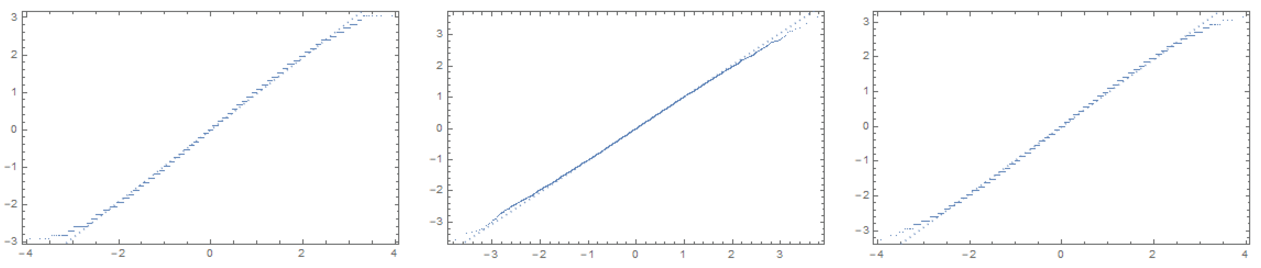
In the same way we have generated all the quantiles and we have compared them with the theoretical values of those of the Gaussian distribution. In each of the cases it can be verified that the values fit the Gaussian model. In the Figure 4 we plot the obtained quantiles list against the quantiles list of a normal distribution for some cases.

In order to better support the results presented, we have represented the cumulative distribution function (CDF) and the results obtained and compared them with those expected in the normal distribution. In the Figure 5 we confront the CDFs of the normal distribution against those obtained resutls.

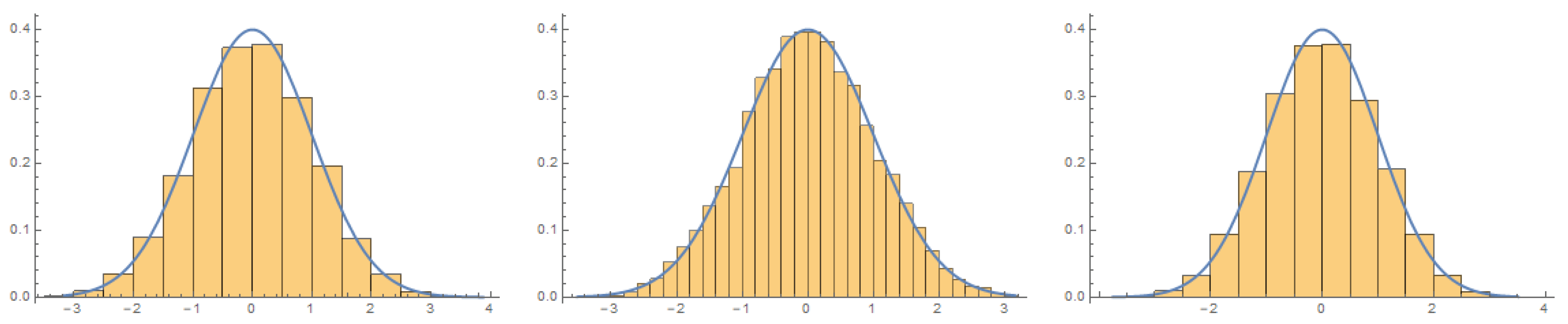
In this regard, it should also be noticed that the histograms of the results obtained have been analyzed and these have been compared within the corresponding histograms of the normal distribution. Continuity correction has been applied since a discrete set of values are being used and we have also been able to verify that the data fit a normal distribution of values. In the Figure 6 we can see how the histograms tend to the normal ditribution CDFs curve.

Although different normality tests were originally used to check if the data fit the normal distribution, as we can see in

Table 6. Distribution fit tests for ${{\kappa }_4}_4$.

Distribution Fit Tests	Statistic	p-Value
Anderson–Darling	0.16486	0.956321
Cramér–von Mises	0.0248859	0.924378
Jarque–Bera ALM	0.214813	0.894745
Mardia Combined	0.214813	0.894745
Mardia Kurtosis	0.00564325	0.995497
Mardia Skewness	0.205783	0.650093
Pearson ${\chi }^2$	13.4135	0.966447
Shapiro–Wilk	0.997609	0.907292

, due to the large number of data, we have opted for the method of the Chi-Square Test, which allows us to check whether or not a model or theory follows an approximately normal distribution.

These described tests have been used to check whether the statistical variables are distributed according to a Normal distribution. A minimum level of confidence has been set to $90\%$ therefore the significance level is set to $10\%$ and according to that level of confidence the sequence obtained has been screened. That is, given a set of values, the Normality tests have been applied to verify whether the data followed a normal distribution or not. The output of these mentioned tests is a p-test. If the p-test value obtained is greater than $90\%$, the sequence obtained is considered valid and otherwise has been discarded.

The proposed generator has been tested for all possible polynomials. All primitive polynomial combinations have been tested using the Mathematica environment. The tests have been performed using Chi sqaure, the Anderson–Darling and Shapiro methods. The results are exemplified in Table 6.

The proposed PRNG [24] has also been compared with the Box–Muller algorithm that was designed as a pseudo-random number sampling method for generating pairs of independent, standard, normally distributed (zero expectation, unit variance) random numbers, given a source of uniformly distributed random numbers. If $U_1$ and $U_2$ are independent samples chosen from the uniform distribution on the unit interval $(0,1)$, then the variables defined as:

$$Z_0=Rcos\left(\mathsf{\Theta }\right)=\sqrt{-2ln\left(U_1\right)}·cos\left(2\pi U_2\right)$$

(12)

$$Z_1=Rsin\left(\mathsf{\Theta }\right)=\sqrt{-2ln\left(U_1\right)}·sin\left(2\pi U_2\right)$$

(13)

are independent random variables with a standard normal distribution.

After having executed the Box–Muller algorithm we have found the following disadvantages.

• According to the results presented in

  Table 7. Evolution of the p-test values obtained, after applying the Chi Square goodness of fit test method to a set of values, for Box–Muller and for our LFSR model.

  LFSR Model	Box–Muller	Pol. Degree	Pol. Degree Ext Field	Number of Values
  0.951123	0.87231	4	4	65,535
  0.90900	0.761121	5	4	1,048,575
  0.90101	0.755181	6	5	1,073,741,823
  0.90012	0.699876	6	6	68,719,476,735

  , we can see that the values of the p-test are better our LFSR model, than in the Box–Muller algorithm.
• The computational cost required to implement the algorithm is much higher.

Another way to improve the accuracy of the Gaussian distribution is to modify the way the m-bit strings are generated. If all the states of the LFSR are used, each cell is used in the generation of n consecutive pseudo-random numbers. Although the fit tests reveal very good results (see Section 4.2), decreasing or removing the amount of numbers affected by the same cell would help to improve the accuracy. Therefore, we propose, as an alternative, to use one out of every m states. More formally, we propose to decimate by m the LFSR output. In this way, the period would be $(2^{mn}-1)/gcd((2^{mn}-1),m)$ giving rise to select $m,n$ such that $gcd((2^{mn}-1),m)=1$ in order to reach the same period $2^{mn}-1$.

In any case, it is important to note that the period is much greater than the range, i.e., $2^{mn}-1\gg 2^{m+lo{g}_2\left(n\right)}$, giving rise to a probability about $0.005$ of generating the same number in $10,000$ values generated.

5. Conclusions

A new Gaussian PRNG has been proposed in this paper. It is based on a unique LFSR, using the same approach than the previous proposals [8,9,10], in order to generate a certain number of sequences of uniformly distributed numbers, needed to apply the CLT. Unlike the previous proposals, no explicit permutations or rotations have been applied to the successive LFSR states. Instead, the PRNG is operated in $GF\left(2^n\right)$ to take advantage of the relationship between the states and sequences generated in $GF\left(2^n\right)$ and $GF\left(2\right)$, that allows to represent the $m-$sequences in $GF\left(2^n\right)$ as primitive interleaved sequences composed by $m-$sequences in $GF\left(2\right)$.

The PRNG, presented in Section 3.2, allows to configure it by means of two main parameters, m (the number of cells in the LFSR) and n (the dimension of $GF\left(2^n\right)$), determining the period as $2^{m·n}-1$, and the range $2^{m+lo{g}_2\left(n\right)}$. The statistical analysis reveals an excellent behaviour when the fit tests are applied.

Finally, this PRNG is a way to keep using LFSR in cryptographic applications where a uniform distribution is not required. Furthermore, as in other applications, the use of LFSRs in $GF\left(2^n\right)$ is motivated by the speed increase that is achieved by generating n bits instead of 1 in each iteration; in this case, the use of the LFSR in $GF\left(2^n\right)$ pursues a second objective: to take advantage of the implicit relationship with n different binary sequences looking for an easier implementation of the CLT. Therefore, the final rate of generating numbers with Gaussian distribution is the same as the rate at which a binary LFSR generates a bit. However, taking into account that the generated numbers are $m+lo{g}_2\left(n\right)$ bits long, the generation speed in bits per second is $m+lo{g}_2\left(n\right)$ times higher.