1. Introduction
The analysis of co-movements in the international financial market has been discussed on a recurrent basis within the financial literature. The subject has raised the interest of researchers especially for the importance of financial contagion on the definition of strategies for risk management in portfolios. Over the past two decades, with global financial integration, investors have also focused on the issue with the objective of diversifying their asset portfolio through cross-border investments.
Regarding the stock market, Heston and Rouwenhorst [
1] suggest international diversification as an effective tool for risk management in equities portfolios. This opinion is shared by Bekaert et al. [
2] who find evidence to support Heston and Rouwenhorst’s [
1] intra-sectoral insights, reporting that country factors are preponderant over industry factors in terms of equity market returns.
However, the evidence reported in Brooks and Del Negro [
3] highlights the growth of interdependence in the international market since the 1990s. Rua and Nunes [
4] suggest that international co-movement presents a heterogeneous pattern over time and frequency, indicating that international diversification tends to generate asymmetric results for long-term and short-term investors in terms of portfolio risk management.
Graham et al. [
5] highlight a strong level of integration between emerging markets and the US market especially over the long-term horizon. The evidence reported in Conlon et al. [
6] also indicates that the gains from international diversification are smaller for long-term investors and the correlation between markets is stronger at low frequencies. On the other side, Das et al. [
7] report a reduction in long-term co-movements between emerging markets and developed markets after the global financial crisis (GFC) of 2008, supporting an international diversification strategy with allocation to markets of different stages of maturation. We conducted a sectorial study, analyzing the interdependence between the five leading global consulting engineering companies—specifically, Arcadis (Amsterdam, The Netherlands), Aecom (Los Angeles, CA, USA), Jacobs (Dallas, TX, USA), SNC (Montreal, QC, Canada), and WSP Global (Montreal, QC, Canada)—based in three different countries. Our study presents two main objectives:
First, to evaluate the intensity of interdependence between the equities considering the spheres of time and frequency, which makes it possible to evaluate whether the periods of economic instability present specific transmission channels over the co-movements between the companies, and whether they vary along the frequencies.
Second, to analyze the effect of financial contagion on a risk measure based on a portfolio composed of the five companies also in the field of time and frequency. Thus, we believe that the evidence obtained will contain important information not only from a theoretical point of view, but also for risk management in portfolios with a well-established planning horizon.
The analysis according to the frequency of fluctuations is also based on differences in the set of information of interest to investors, according to their planning horizon. While short-term cycles are strongly influenced by specific noises in sectors/assets that are strengthened from traders’ short/long positions. The medium- and long-term cycles are induced by systematic news, which tends to amplify the co-movements to the extent that there is a reduction in the amount and complexity of information available Chakrabarty et al. [
8]. In this context, the wavelet transform becomes especially useful for modeling the co-movements between assets, as it is able to capture the synchronicity/contagion between assets in the time and frequency domain.
To achieve the first objective, we use tools based on wavelet analysis to model the market returns of companies between 9 January 2014 and 9 December 2020 in order to verify the evolution of co-movements between companies in a variant structure in the domain of time and frequency. Specifically, we based the analysis on the approach proposed by Aguiar-Conraria et al. [
9], and also discussed in Matos et al. [
10], using the wavelet partial coherency (WPC) to identify the co-movements among pairs in the domain of time and frequency. Partial phase-difference and partial gain measures are also adopted in order to identify lead–lag relationships between pairs at different frequencies. These tools allow us to assess the presence of financial contagion over time among companies in short-, medium- and long-term cycles, a crucial differentiation to subsidize the decisions of short-term and long-term investors.
To reach the second objective, we follow Rua and Nunes [
4] who proposed the value at risk (VaR) ratio analysis in the time frequency domain. The authors start from matrices of variance and covariance computed from the wavelet analysis, in order to construct a ratio for the volatility of a specific portfolio with the covariance observed among the assets in the numerator and assuming covariance statistically equal to zero in the denominator at each time-frequency locus. Based on this VaR ratio it is possible to identify whether the financial contagion between the companies contributes to the increase or reduction of risk in the portfolio in a structure also variant in time and frequency. We further believe that the distinction of analysis in terms of time and frequency has the potential to provide insight into portfolio risk management for funds and investors with respect to the horizon (frequency) and period (time) of exposure to assets.
It is important to highlight that alternative methods have been developed in the literature over the last decade to measure spillovers among financial assets as well as to identify the systematic risk associated with the construction of investments portfolios. The directional spillover model (DY)—according to Diebold and Ylmaz’s [
11]—is used to measure contagion between financial asset returns (Kang, Mclver and Yoon; Akhtaruzzaman, Boubaker and Sensoy, [
12,
13]), discuss the methodology identifies spillovers from a generalized vector autoregression (VAR).
A natural extension of the DY model is the application of spillover indexes in the dynamic context from the Dynamic Conditional Correlation-GARCH model (DCC-GARCH), in which the covariance matrix between assets is estimated in a time-variant approach, as discussed in Gamba-Santamaria [
14]. However, these models rely on the assumption of stationarity in covariance to obtain consistency in the estimators, and do not present a flexible structure in the frequency domain, which makes it unfeasible to adopt them in the present case. Wavelet analysis has been widely used to identify transmission mechanisms between assets and financial assets, such as currencies, commodities, market indices and stocks. Jiang and Yoon [
15] indicate that the price of a barrel of oil has heterogeneous effects on the financial markets of oil-exporting countries relative to oil-importing countries, indicating more pronounced co-movements between stock prices of oil-exporting countries and oil prices. Pal and Mitra [
16] find evidence that co-movements automobile stock return and oil price only in low frequencies (256~1024 days) only in periods of high economic uncertainty, with stock prices and oil price in a pro-cyclical relationship, evidence against the hypothesis that diversification between both asset classes reduces portfolio risk.
The effect of the Covid-19 outbreak has also been the subject of study based on wavelet measures used in Wu et al. [
17], that indicate that the uncertainty associated with the expansion of the pandemic in global terms has affected the American financial market in a heterogeneous way in the domain of time and frequency. Choi [
18] conducted a pioneering study disaggregates the analysis in terms of the US stock market sectors, and attested to the influence of COVID-19 on the share price in all sectors from the wavelet coherence. Goodell and Goutte [
19] report that the increase in the number of deaths recorded by COVID-19 is associated with the increase in Bitcoin price in a short-term horizon (4~8 days) during the initial period of the pandemic. Causality, however, is not verified in frequency bands equal to or greater than 8 days. Based on the sectorial data for the S&P 500, Matos, Costa and Silva [
20] identify that the energy sector anticipated the oscillations in the other sectors during the financial crisis triggered in March 2020.The article is composed into the following sections:
Section 2 presents the wavelet methodology.
Section 3 we present the descriptive statistics of the actions and the empirical exercise. Finally,
Section 4 presents a discussion and the final considerations are made.
3. Empirical Exercise
3.1. Data and Descriptive Statistics
The study used daily return data adjusted for dividends from the world’s five leading consulting engineering companies (Jacobs, Aecom, Arcadis, SNC Lavalin, and WSP Global). The data was extracted from the
Investing.Com website and covers the period from 9 January 2014 to 9 December 2020, resulting in 1731 daily observations for the six-year period evaluated. We follow Mink [
24], approach, considering the return on shares in local currencies.
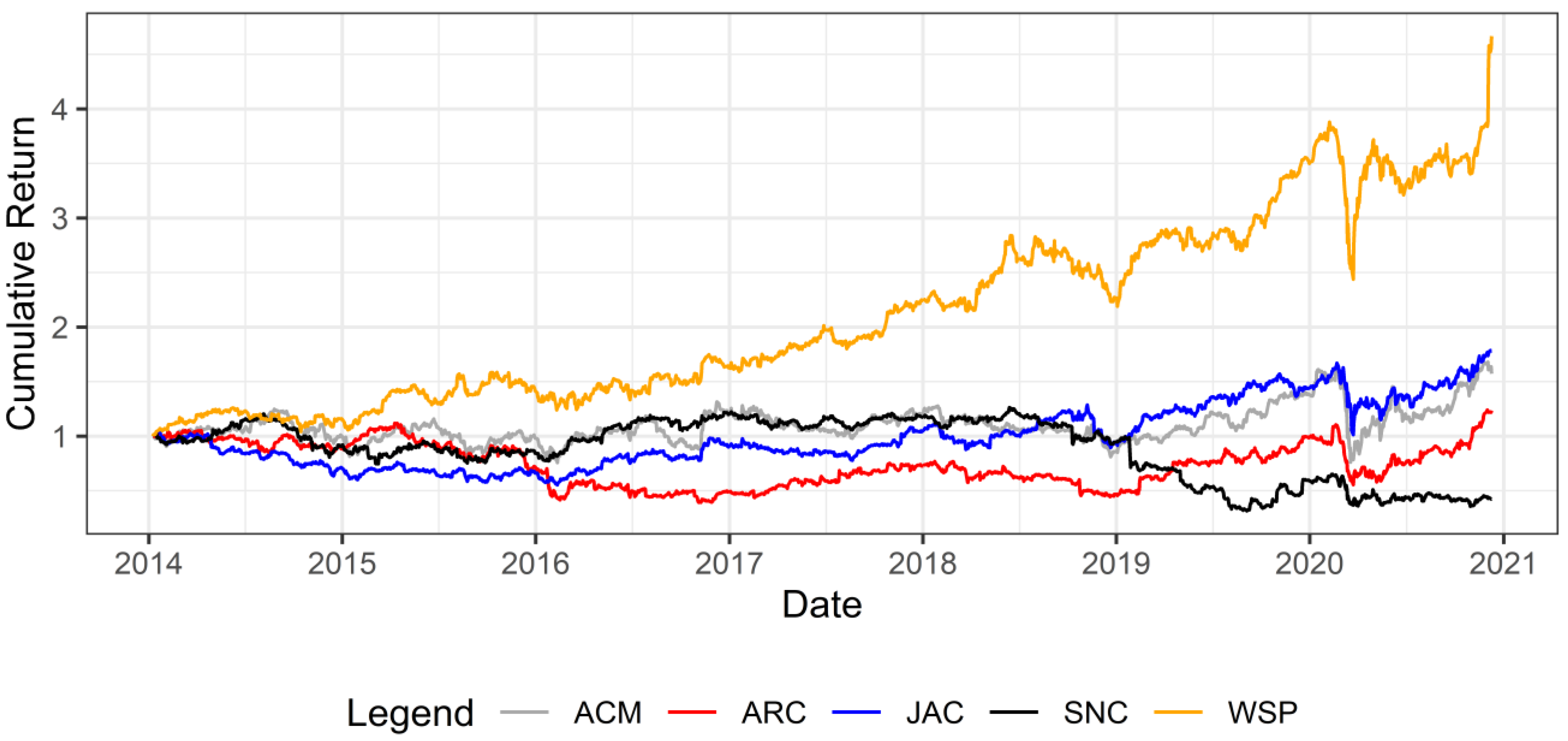
Figure 1 reports the evolution of the accumulated return on shares during the sample interval, the company WSP presented the best performance, with a gain of 367% in market value, while the company SNC was the only company with net loss between 2014 and 2020, with a reduction of 57% in its market value. The other companies obtained a moderate gain in market value, oscillating between 23% (Arcadis) and 78% (Jacobs).
According to
Table 1, with the exception of the WSP, all other companies reported a distribution of daily returns with negative asymmetry, indicating a higher relative frequency of small gains, but with more extreme values to the left of the distribution. The daily returns have a positive excess of kurtosis (fourth central moment of the distribution), indicating the incidence of more pronounced extreme values, indicating a higher degree of risk in this asset group.
In
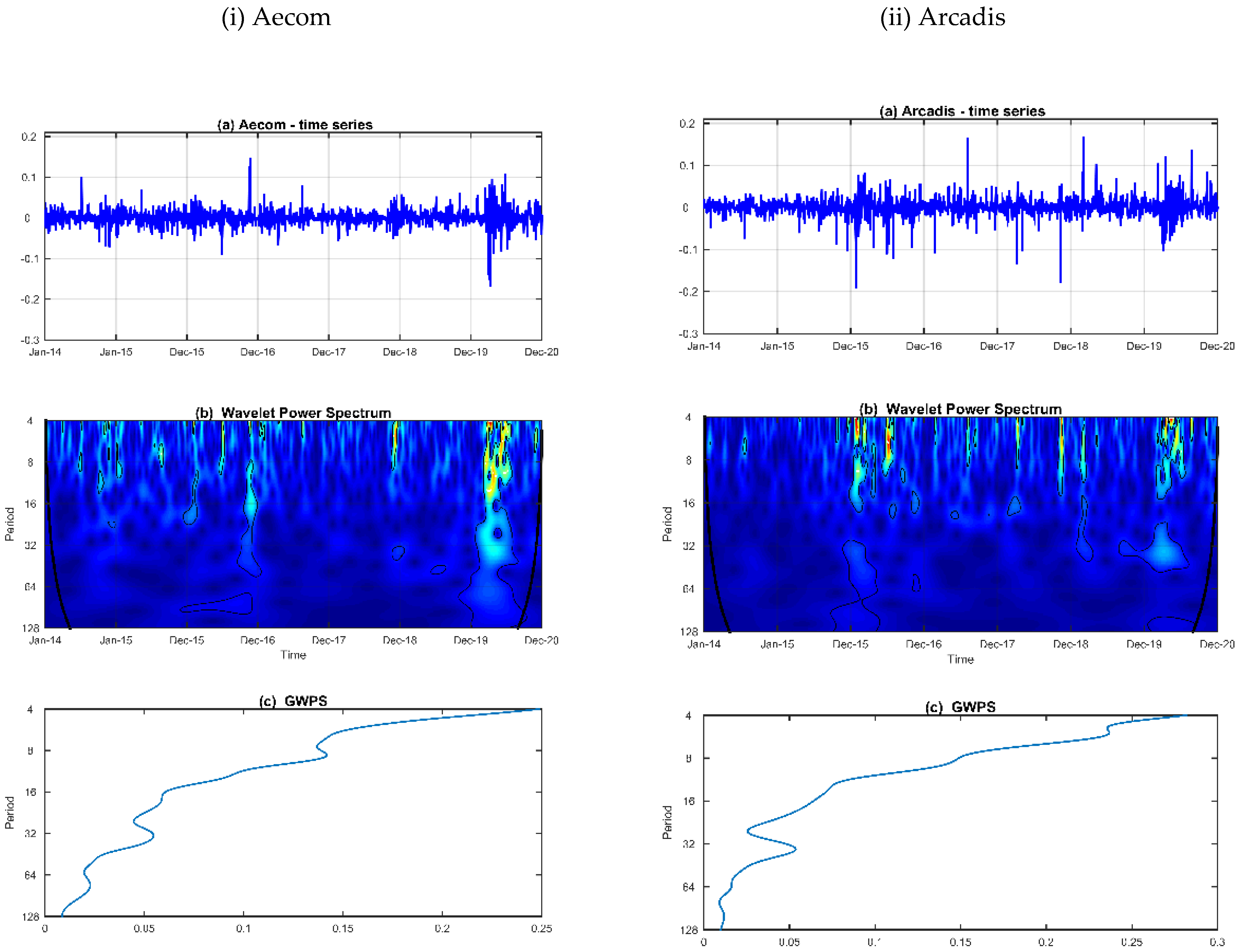
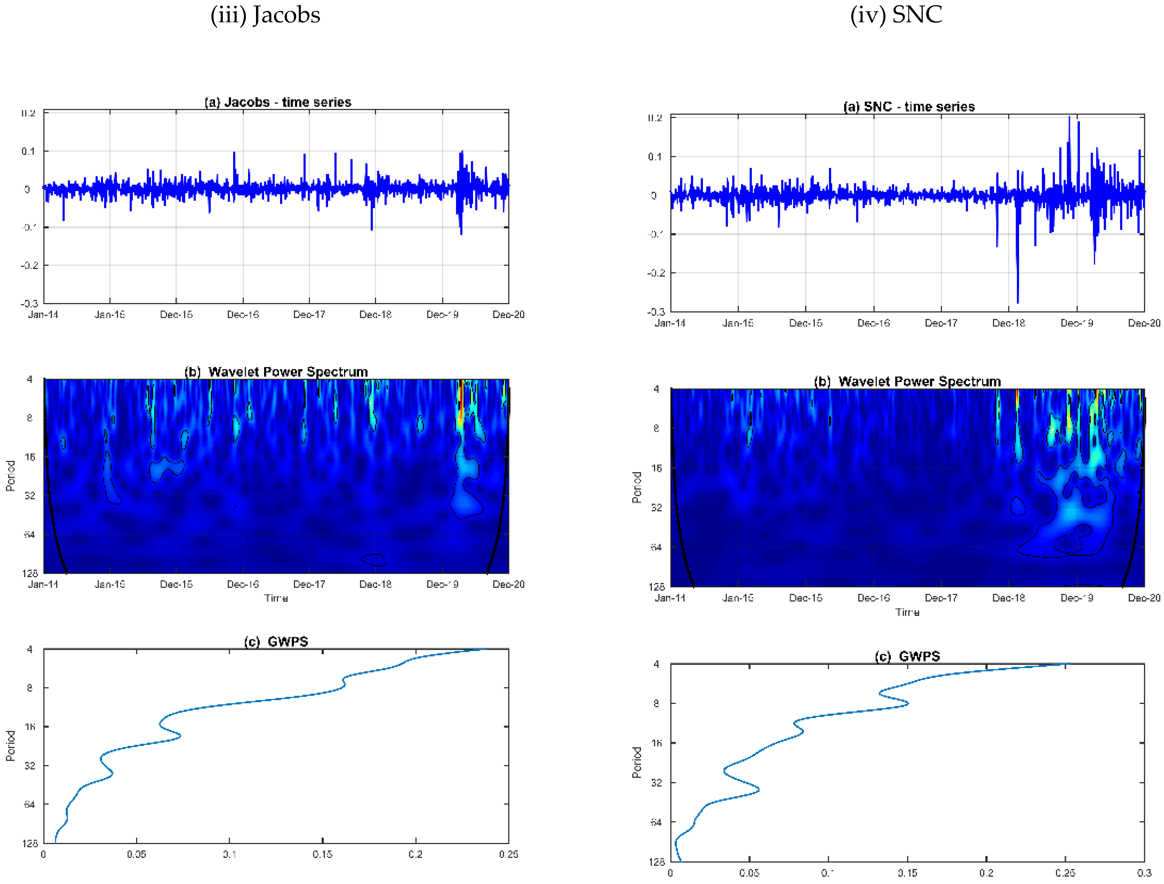
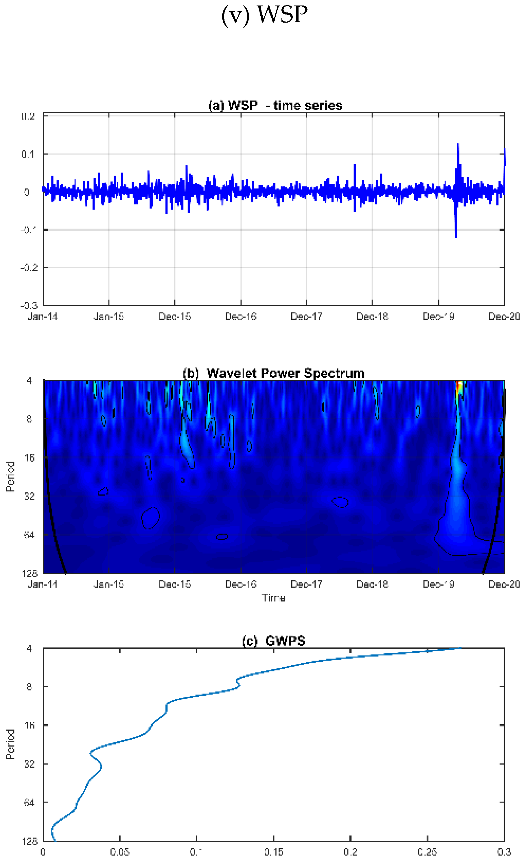
Figure 2, we plot the time series (top columns), the wavelet power spectrum (middle columns) and the global wavelet power spectrum (bottom columns) for each firm. The wavelet power spectrums (WPS) provide the variance of series at each time-frequency locus (time is on the horizontal axis and the frequency, in days, on the vertical axis) and the global wavelet power spectrums (GWPS) offer the average wavelet power for each frequency (vertical axis).
The GWPS (c) for each series indicates a strong volatility in the return structure over the higher frequency’s bands (4~16 days), with irregular’s spikes of variance at medium-term cycles (16~32 days) and non-evidences of higher episodes of volatility are observed for frequencies greater than 64 days. Others interesting findings are showed in the WPS charts (b) the volatility gets stronger between 2015–2016 and 2019–2020. The first interval is demarked by the stock market China crash and the second period is mainly related with the COVID-19 outbreaks. Over both time intervals the variance decreases across the frequency’s bands but it remains high for frequencies greater than 32 days only in the interval 2019–2020.
Regarding of the individual series, the WSP (a) indicated a higher volatility in the market return for Arcadis between 2015–2016, where the variability remains strong until 16 days frequency bands. During the 2019–2020 we highlight a more pronounced episode of volatility for Aecom’s market return, with a more persistent area of variance between the 8~16 days frequencies.
3.2. Results
In order to control the effect of global disturbances on co-movements among consulting engineering companies, the variation in spot prices of the WTI type oil barrel was adopted as a proxy for global economic activity. Dong et al. [
25] find evidence that oil prices are a coincident indicator of global economic activity, especially at high frequencies, main horizon of analysis in this article.
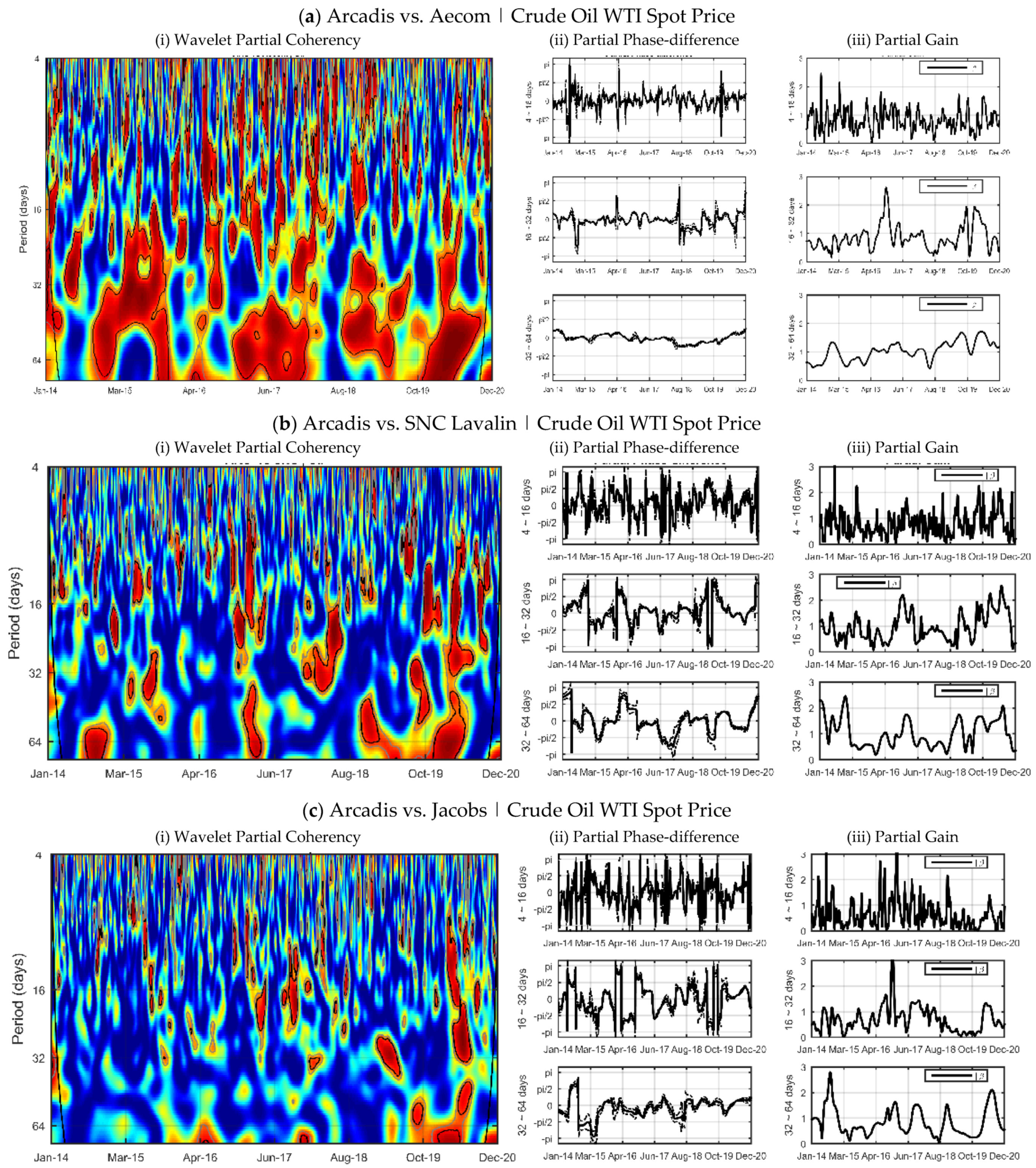
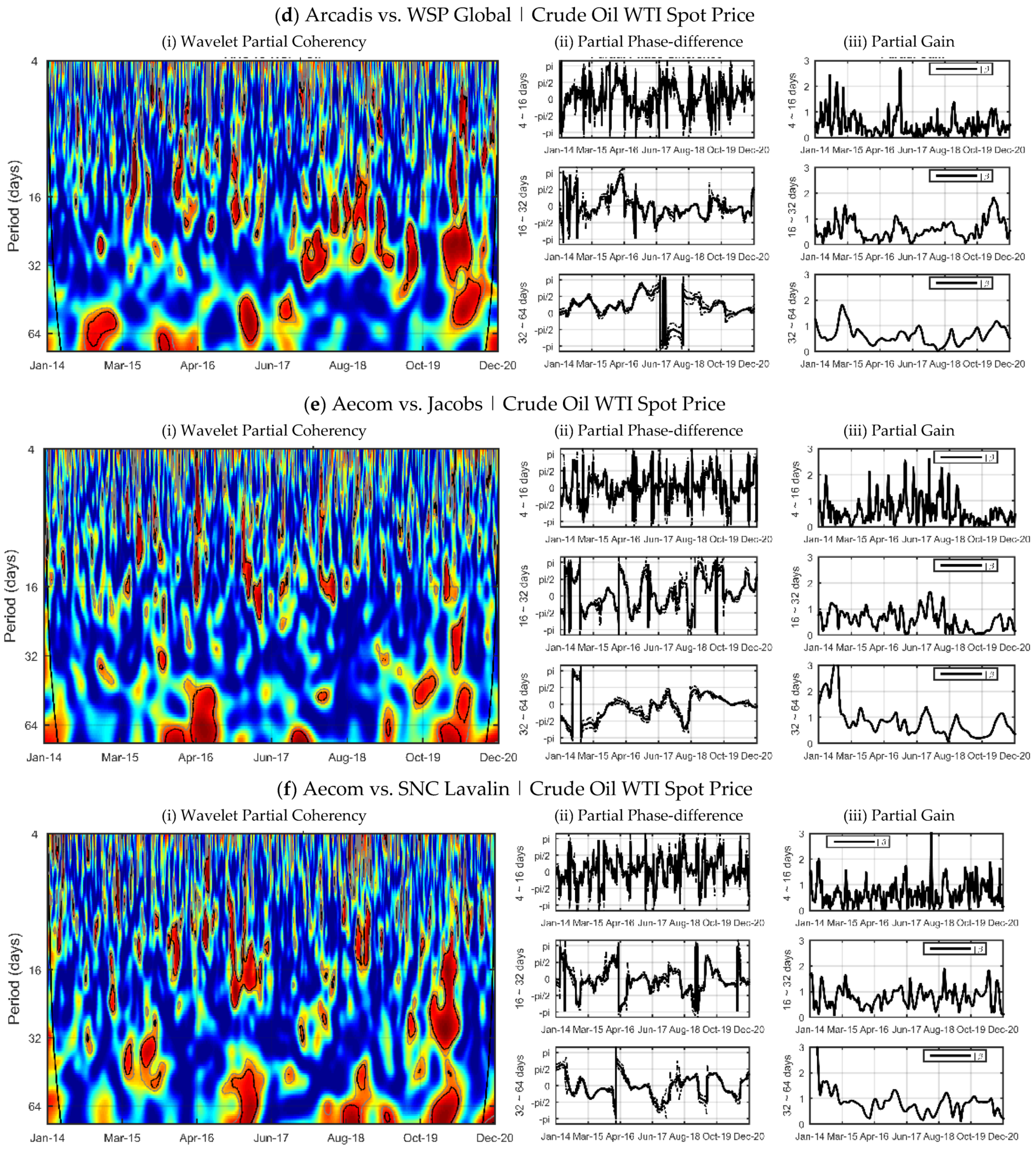
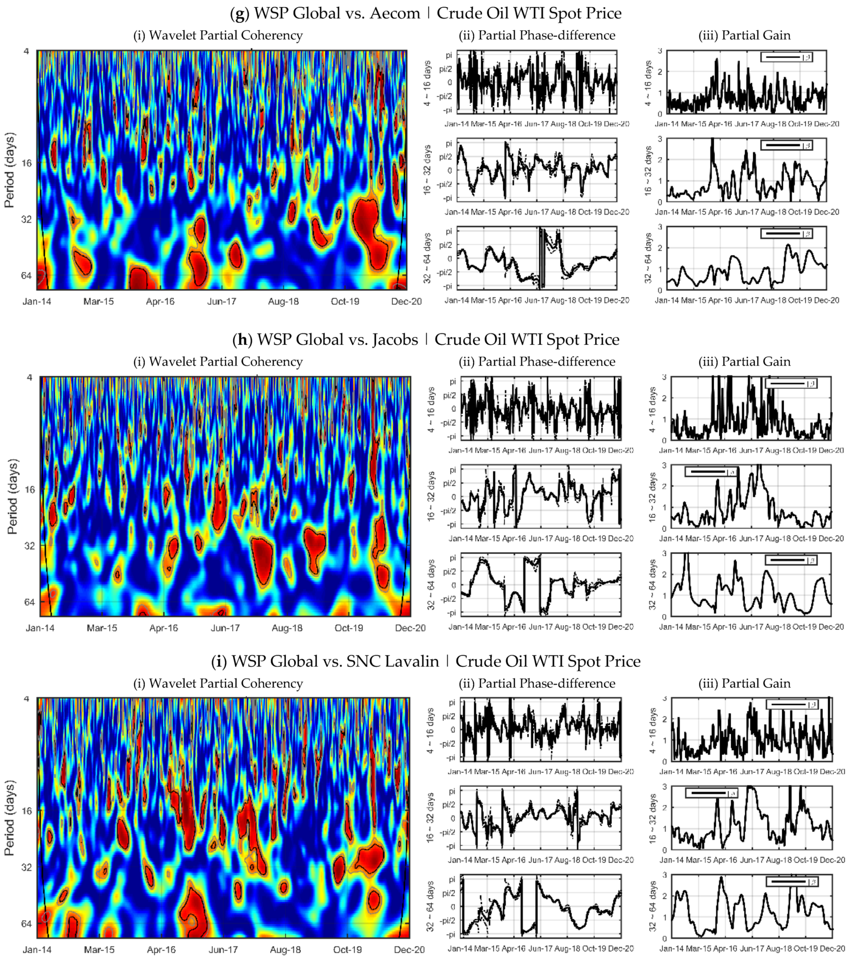
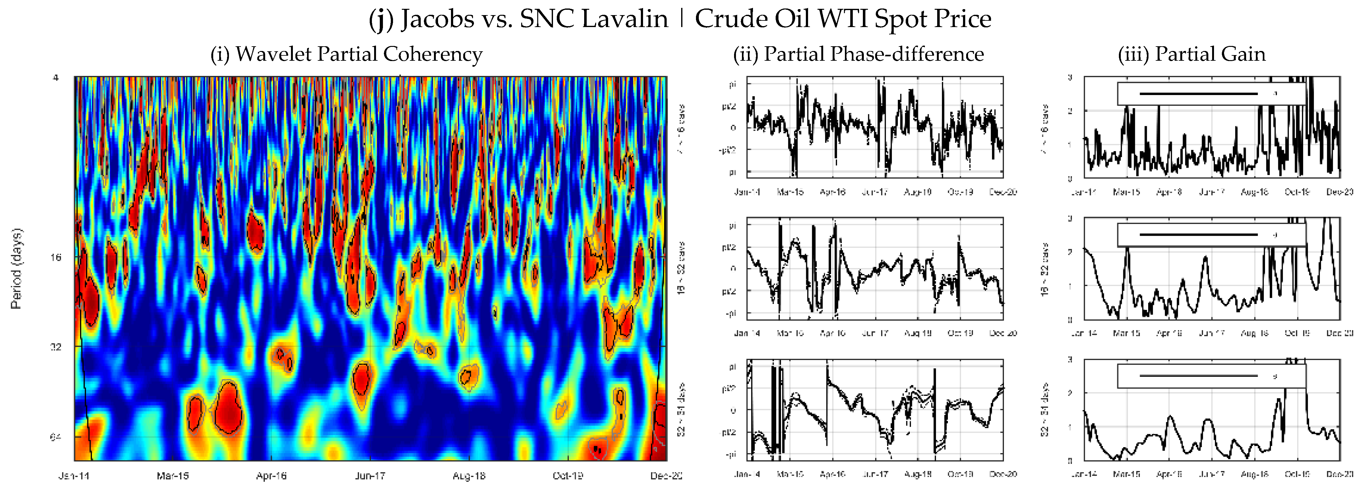
Figure 3 shows the partial wavelet coherency—PWC heat maps between companies, the horizontal axis reports the time interval while the vertical axis refers to the frequency of the cycles, which is given in days. Regarding the degree of synchronization between the companies’ cycles, the ratio is as strong as the hottest the color on the map. The partial phase-difference and partial gain analysis were segmented into three cycle frequencies: short cycles (4~16 days), medium-term fluctuations (16~32 days) and long-run relationships (32~64 days). From a theoretical point of view, the horizon partition follows closely the literature, with the short-term horizon capturing weekday effects Sun and Tong [
26], the medium-term horizon containing the turn-of-the-month effect Khaled and Keef [
27], and the long-term cyclical component translating relationships with a higher degree of persistence. On the practical side, we believe that the differentiation of the horizon in terms of frequency produces an important set of information for different types of investors, depending on their planning time horizon.
In general, the evidence supports the importance of time-dependent analysis. Companies’ returns presented more frequent and long-lasting high synchronization regions at low frequency (32~64 days), with irregular periods and low synchronization stability at short term horizon (4~16 days).
In the low frequency horizon (32~64 days) regions of statistical significance with at least three months duration were found for all ordained pairs. Regarding time, synchronization between cycles was stronger during the 2015–2016 and 2019–2020 intervals. The first interval is associated with the period of China’s market crash, which presented a 40% decrease between June and August 2015. Fang and Bessler [
28] highlights that the bear market in China negatively influenced the main Asian markets, generating a global chain effect. The second interval, on the other side, suggests an increase in synchronization among assets even before the advent of the pandemic, reflecting a bullish cycle in developed markets observed over the past few years.
In the medium-term frequency (16~32 days) the regions of strong synchronization become more irregular. However, our results indicate the existence of co-movements at the final sample interval in all ordered pairs. We believe that this result is related to the economic crisis generated by the COVID-19 pandemic, which has accentuated the synchronization among companies. To a lesser extent, there are frequent cases of high synchronization over the years 2016 and 2017.
We did not find any stable high synchronization region at high frequency (4~16 days). The strongly irregular pattern in all partial difference-phase pairs confirms the statistical independence between the short term cycles of company returns during the 2014–2020 interval.
This evidence supports the relationship between horizon heterogeneity and information heterogeneity in defining market cycles, suggesting no spillovers among assets at high frequency, potentially due to idiosyncrasies in news affecting the short-term trend in the returns of these stocks Chakrabarty et al. [
8].
From an individual point of view, Arcadis reported higher relative levels of synchronization with other companies. Arcadis and Aecom presented robust synchronization standards during the 2014–2015, 2017, and 2018–2020 intervals. For the last period, Arcadis reported a lag-relationship with Aecom (Partial Phase-difference (), with Aecom’s return variations at low frequency causing a pro-cyclical effect on Arcadis returns superior to unity (Partial Gain > 1). SNC led Arcadis’ long term cycle between October 2019 and April 2020 (interval where PWC was significant in low frequency). In the medium-term horizon, the WSP company also pro-cyclically led Arcadis in the medium-term frequency (16~32 days), the partial gain oscillated around the unit.
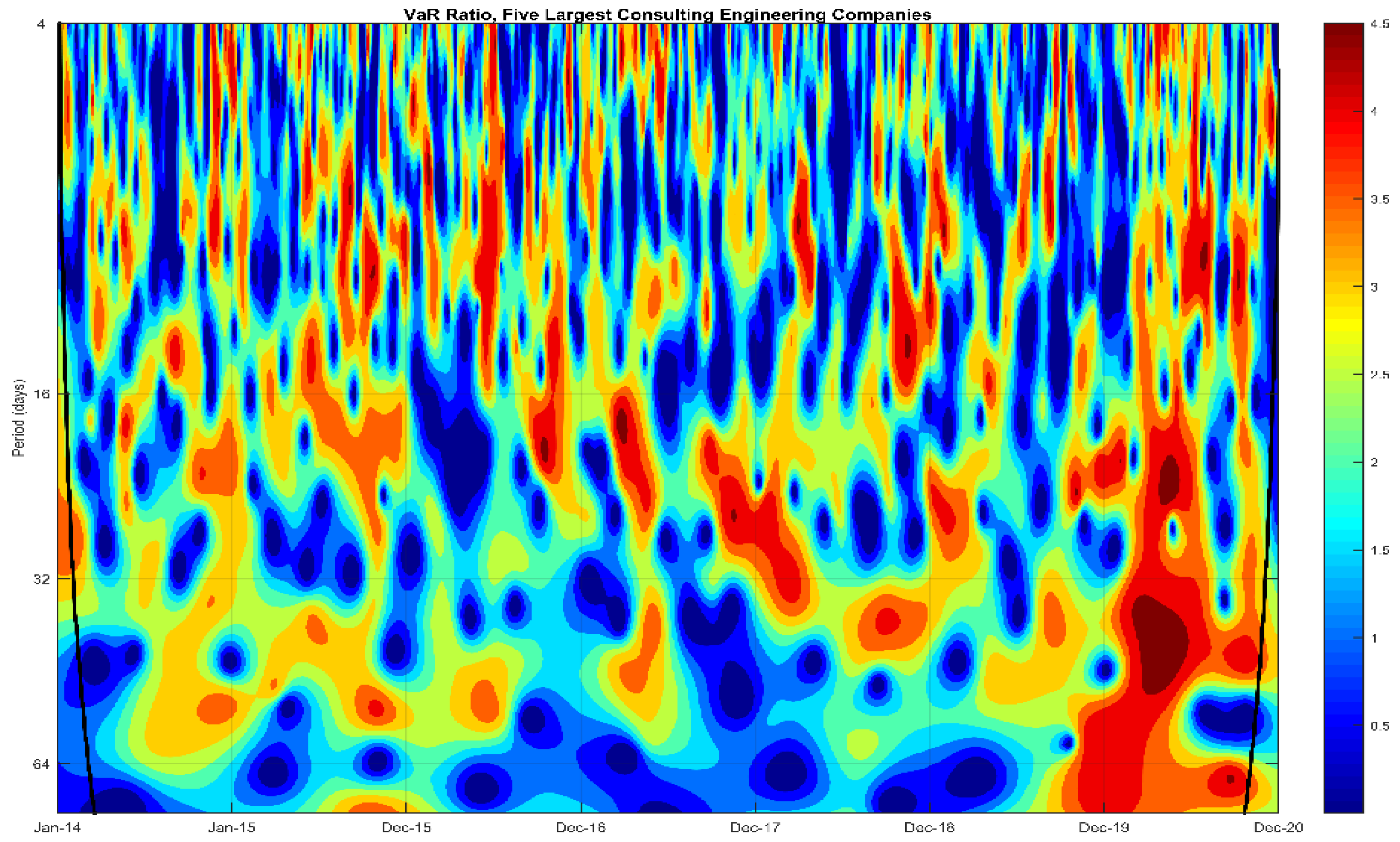
Considering an equally-weighted portfolio comprised by the market return of the five companies, the VaR is an important instrument for risk assessment that quantifies the maximum loss of a portfolio not exceeded with a given probability over a period of time (Rua, 2009). We follow the approach presented in Rua and Nunes [
4], by computing the ratio between the VaR with and without assuming co-movement among the stocks in time-frequency space. Thus, areas where the VaR ratio are greater than one indicates that the co-movement among the assets comprising the portfolio increases its risk.
The VaR ratio test (
Figure 4) exhibits some interesting evidences about the co-movements among the assets. The ratio is predominantly greater than one for all horizons of cycles, the average ratio at short-term cycle was 1.33, increases to 1.46 at medium-term cycle and for 1.46 at long-term cycle. So, we highlight a 10% growth in the risk for fundamentals investors relative to the risk associated for short-term allocations locus.
When we evaluate the VaR ratio at the specific intervals of highest volatility in return on assets (2015–2016 and December 2019 through March 2020) according to the WPS results, the findings also report a higher relative risk level for the frequency between 32 and 64 days (long-term cycles). For the first interval, we highlight a 2.16% increase in portfolio risk over the long-term horizon relative to the highest frequency (VaR ratio of 1.42 versus 1.39).
The effect of financial contagion among assets on portfolio risk is even more pronounced for the interval from December 2019 to March 2020 (period of maximum uncertainty associated with the COVID-19 pandemic), with a 38.6% increase in portfolio risk in the long-term frequency (VaR ratio of 1.97 for the frequency between 32 and 64 days) relative to the short-term frequency (VaR ratio of 1.42 for the frequency between 4 and 16 days).
Our results are consistent with the evidence reported in Rua and Nunes [
4], who observed: (i) an 80% increment in the VaR ratio at low frequencies in a portfolio composed of the German, Japanese, UK and US market indexes between January 1973 and December 2007; and (ii) higher intensity in the co-movements in periods of economic crisis, such as the 1987 US stock market crash and the technology bubble episode in the late 1990s. Note however that the results are not directly comparable, insofar as the authors used monthly market returns while our analysis is conducted using daily data.
4. Conclusions and Suggestions
The analysis of co-movements and the value at risk between shares is a relevant factor for the risk management and return maximization of an investment portfolio. However, it is also relevant to consider that investors of different profiles have a heterogeneous degree of exposure in terms of the frequency level of oscillations and co-movements between assets. In this case, obtaining disaggregated evidence in terms of time and frequency is essential for the optimization of the portfolio, modeling the associated risk according to the horizon of interest of investors.
To consider this fact, we evaluated the co-movement among the market returns of the five main consulting engineering companies in the world (AECOM, Arcadis, Jacobs, SNC Lavalin and WSP Global) for the period from 9 January 2014 to 9 December 2020. The study is pioneer as far as we have knowledge by using wavelet based methods for a sample of intersectoral companies in international terms. This disaggregation framework has the potential to contribute to a new round of discussion on the relative importance of industry effects and national effects, considering the time and frequency space.
Although we have used the price of a barrel of spot WTI oil as a proxy for the business cycle, we recognize the possibility of the variable’s limitation in not capturing the influence of macroeconomic disturbances on market conditions. In this sense, the addition of variables associated with GDP, economic uncertainty and interest rate spreads, for example, would be more consistent indicators, however the unavailability of the first two indicators on a daily basis makes it unfeasible to add them, while the latter presents extremely low volatility in the very short term. One way to overcome such difficulties is to work with market returns on a monthly basis, but we consider that the associated gains do not compensate for the cost of the loss of information associated with market behavior over the planning horizon of short-term investors for the present case. The empirical evidence indicates a growth in the coherence between market pairs over the period 2015–2016 over the short and medium-term cycle horizon. We consider that this result is potentially associated with the Chinese market crash of 2015, which triggered a wave of turbulence especially over the commodities market, accentuating the uncertainty in the market during the period. However, the COVID-19 outbreak period triggered a sharp increase in co movement among companies, presenting a higher degree of persistence, given both the greater amplitude of the areas of significance for consistency among the pairs and the incidence of consistency regions in low frequency cycles (32~64 days). Therefore, our results support the existence of a high systematic risk in the sector in periods of market crash, indicating the preponderance of industry effects in periods of financial instability.
Value at risk wavelet-based modeling indicates that international diversification based on a portfolio of consulting engineering companies is flawed by reducing portfolio risk. Value at risk was on average higher than 1 for all frequency bands (short, medium and long term). In relative terms, value at risk was higher in periods of turbulence, and in frequency, value at risk was higher for long term cycles. This evidence indicates that there are no benefits from diversification, especially in periods of great uncertainty and for long-term investors.
