Models of Wealth and Inequality Using Fiscal Microdata: Distribution in Spain from 2015 to 2020
Abstract
1. Introduction
- Distributions. Many researchers have tried to achieve a comprehensive unique and universal fit of the observed density or distribution functions with: biparametric (lognormal, gamma, Weibull) distributions, triparametric (generalized gamma, Singh-Maddala or Dagum) distributions [28], and pentaparametric (generalized beta) distributions [29]. Economists have preferred lognormal distributions [30], while statisticians [31] and econophysicists [32] have shown the utility of gamma distributions. Gibbs’ distributions have been used to fit cumulative data.
- Models. They have been investigated by scholars who believe that it is plausible for a unique simple physical law or a stochastic model to explain the observed regularity. For a complete review of the models, see [18].
- Subpopulations. Some studies, interested in the design of effective policies, have attempted to adjust the density function as a mixture of component subpopulations of wage earners, pensioners, etc. [33].
- What are the underlying causes of the distribution?
- How is it possible that such skewed distributions are observed in competitive capitalist markets that should be efficient?
- What are the processes governing the constitution of existing subgroups, and their influence on wealth and income distributions?
- Determine which of the income and wealth variables best determines the form of a universal law of wealth distribution provided there is access to microdata.
- Identify the subgroups existing in a society whose mix determines the wealth distribution and find the distribution of each subgroup in the case of Spain.
- Model the wealth generation processes of the subgroups.
- Quantify the deviations and errors that occur in estimating income and wealth caused by the involuntary use of variables with partial or biased information.
- Explain the emergence of the shape of the upper tail of the wealth distribution.
2. Methodology
- 1.
- Data collection. We used detailed data from the declarations presented to the Spanish State Tax Agency (AEAT): taxpayer census, information submitted by public bodies (e.g., cadastre), tax (personal income tax, corporate tax, inheritance tax) self-assessments, as well as informative declarations submitted by insurance companies and financial institutions (the authors are solely responsible for their conclusions, which have not been reviewed by AEAT).While some authors [26] have already used income tax microdata, this study increases the level of detail. We selected the variables of interest from many tax declarations, including, for example, the gross tax base from Income Tax Form 100; data on partners and % participation in other companies from Corporate Tax Form 200, and data on assets and liabilities from other forms, such as F 720, F 174, F 196, F 714 and F 189. All the forms and variables used are described on the AEAT web page (AEAT, 2020).The number of taxpayer declarations in an average year (2018) include 19.98 million for income tax, 1.59 million for corporate tax and 207,225 for inheritance tax. A total of 94.7 million current accounts, and loans worth around 139.5 million euros are processed annually, using several hundreds of millions of data items sourced from the Spanish cadastre and from the informative declarations provided by financial institutions. These data are included in the AEAT annual reports [36].We have studied three variables:
- (a)
- Income. Gross tax base, declared on Form 100.
- (b)
- Assets. This is the sum of direct assets (value of property, financial products, deposits, insurance policies, shares in listed companies, etc.) and indirect (or corporate) assets, that is, the value of the % participation in the assets of non-listed companies.
- (c)
- Net worth (). Assets minus passives liabilities (loans and accounts payable) is the sum of two components (direct net worth) and (indirect net worth).For each inhabitant, indexed by i, , ( 59,73 M),where is the set of direct assets belong to inhabitant i and is the set of companies in which inhabitant i has a share.
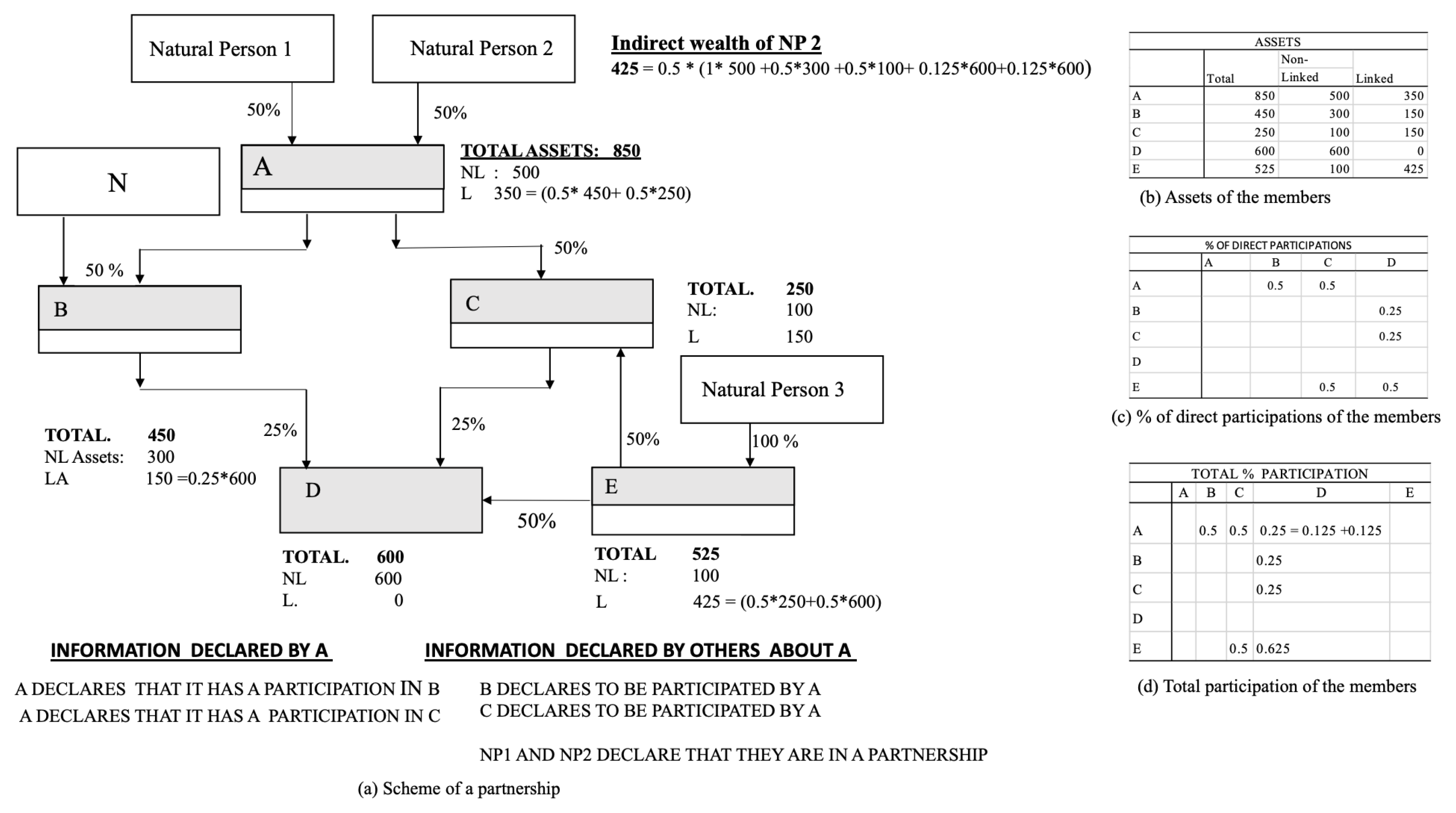
The calculation of the components of indirect wealth is complex because taxpayers may or may not to have participations in non-listed companies, which may or may not hold shares in other companies and so on. It is calculated according to two different processes explained using the toy example in Figure 1 with three natural persons and six companies {N, A, B, C, D, E}.Following the example of Natural Person 1, we calculate the direct wealth of taxpayers from the declarations presented by the taxpayer and by others (e.g., financial institutions). Indirect wealth is calculated by accumulating the market value of participations in non-listed companies {A, B, C, D} that are downstream in the flow of relations between participations. In this example, Natural Person 2 is a shareholder of A only. The relationship between company A, Natural Person 1 and Natural Person 2 is declared by A on page 2 of Form 200. The relationship between A and {B, C} is declared by A on page 24 of Form 200 and includes the % participation and its value. This information can be crossed with the information provided by B and C.The process is divided into two phases:- (a)
- Calculate the % participation of each taxpayer in each company. This is a network-based calculation using the information provided by companies on page 2 and 24 of Form 200. For example, the % participation of Natural Person 1 in D is output by adding two components along paths A-B-D and A-C-D with a total of 0.25, as illustrated in Figure 1d.
- (b)
- Calculate the target variable (assets or net worth). We used balance-sheet data declared on Form 200 to output, for each network node, two set of values: (a) linked assets and liabilities; (b) non-linked assets and liabilities (that is, the balance-sheet items that appear due to company participation in other companies) as illustrated in Figure 1 for the example.Now,where is the set of companies in which inhabitant i has a share, is the set of all the paths from i to c and l is a company along the path p.The indirect net worth of a taxpayer’s participation in a company is the sum, for the companies, indexed by c, in which it has a share, and for all the paths, indexed by p, that connect the taxpayer with a company, of the product of % participations multiplied by the non-linked net worth () of these participations in the L companies along a path. The non-linked assets (referred to in Spanish as “no vinculados”) are calculated using data from Forms 200 and 220, including the balance sheet items. A close approximation to the linked value can be calculated from the balance sheet by deducting the value declared under items 00118, 00153, 00160 referring to assets and items 00223, 00238, 00243 referring to group and partner companies from the company assets. It was decided that the value of a taxpayer’s urban property is, in each case, the maximum of three available values: (a) the value declared on Form 714 (Boxes A, A1, C, D and M), the cadastral value of the property plus the value declared on Form 720 [37].
- 2.
- Variable selection. We collected and studied the descriptive statistics of candidate variables: income, assets, net worth, net worth of the net holders of wealth, etc. We then examined the limitations derived from technical taxation issues, such as exemptions from declaration at specified wealth intervals or special regulations, and decided that the best theoretical option for gaining a clear understanding of reality would be total value of assets.
- 3.
- Decision on the optimal binarization of the data. We decided the optimal binarization strategy. The wealth range is with a mean, , of the order of 5 × 10 within which both high and low incomes have to be closely scrutinized.
- 4.
- Analysis. Although different distributions have been studied (see Section 1 above), biparametric distributions have been most often used in meta-analysis. Normal, lognormal, Pareto and, occasionally, gamma distributions have been used to compare the quality of the fits against distributions with more parameters.As a reminder, Kleiber and Kotz [38] studied at length the types of this family of distributions in which Mandelbrot [39] singled out a strong form, expressed in Equation (3), where is a scale factor, and the value of is not determined.
- (a)
- Pareto I distributionor alternatively, using the survival function, which is the complement of the distribution function:Pareto’s law [40] considers the variable in the positive range (even in the knowledge that there are people who are net debtors, he studied wealth above the survival threshold), where the higher the Pareto index, the smaller the proportion of very rich. The value output by modern empirical studies is close to 2, bigger than in older studies [19,41].
- (b)
- Lognormal distributionThis type of distribution is intuitively applicable and is endorsed by Gibrat’s research, because the distribution of any manifestation of wealth is universally asymmetrical [42].
- 5.
- Analysis of the population mix. Pareto [49] observed that “society is not homogeneous”. This ledthem to think that inequality would be understood by studying the shape of the distribution of the total population. We now know that this intuition was true and that the Pareto index is an indicator of this form. While in a conventional exploratory study, we have to infer the number of subpopulations in the mix, knowledge of multiple covariates for each taxpayer, like age, activity, and income details, as well as expert knowledge, greatly facilitates the identification and choice of the “natural” subpopulations.In a mixture experiment, the experimenter selects a number of different mixtures and varies the proportions of two or more of their components. If we call the number of components q, and is the proportion of the i-th component, then the value of each component is between 0 and 1, and its sum is 1. Due to the constraints, the geometric description the factor space that contains the q components consists of all the points within the bounds of a () simplex. The points inside the rectangle have possitive components, and its centroid describes the mixture with an equal proportion of their components.Having identified the factor space, we could ascertain which mixture of populations best explains the empirically observed distribution. If society is made up of K subpopulations and the density function of each subpopulation is , where is a parameter vector, then the density function of the population iswhere is the proportion of each population, with , and its sum is 1. The population density of the model is approximated by estimating the parameter vector, without knowing to which of the groups each member belongs. If the number of subpopulations is known, the parameters can be output by maximum likelihood, where the most common options are the EM algorithm [50] or Bayesian methods.
3. Wealth Distribution in Spain
3.1. Data Collection
3.2. Variable Selection
- 1.
- Income. Some problems are inevitable:
- (a)
- Low incomes (<€22,000) are exempt from declaration.
- (b)
- The comparability of different studies is limited because these variables are defined legally, and there are special income attribution schemes in each country.
- (c)
- The tax base may be negative.
- (d)
- Tax fraud related to salaried income is easier to detect than for income of professionals or the extremely wealthy.
- (e)
- The data distribution may be contaminated due to the tendency to defraud [52].
- (f)
- The distribution mode for low incomes is sensitive to binning. For example, with a €100 grouping, the mode is situated in the interval (€) [13,800–13,900] (# 73,822 taxpayers). For a €1000 grouping, the mode is in the interval [10,000–11,000] (# 537,999). For a €10,000 grouping, the peak is between [50,000 and 60,000].
- (g)
- The use of income introduces a bias because workers may have mortgages, or assets, placing them in a completely different situation to others, with a similar salary, that are or are not homeowners.
- (h)
- 2.
- Net worth. Its associated difficulties are:
- (a)
- Values may be negative if there are net debtors.
- (b)
- Although possible, it is very difficult to calculate. The problems are:
- All the tax data on declared incomes and debts are required for its calculation.
- Details contained in the corporate tax declaration that are not available in all countries are required to calculate indirect equity, that is, shares owned in unlisted investee companies.
- All the assets of the companies owned by taxpayers have to be transferred to the current price value.
- The declared corporate tax values have to be adjusted for each company due to different amortization rates that are acceptable under accounting rules, and the process is very complex [37].
- Access to all the direct and indirect liabilities (loans and debts) of each taxpayer, even if assumed by the company in which the taxpayer has a share, is required.
- 3.
- Total assets. This variable is more detailed than income, is always positive and does not have so many technical issues (from the viewpoint of accounting and data accessibility) as net worth.
3.3. Decision on Binarization of Data
3.4. Analysis of Wealth
3.4.1. Variable Distribution
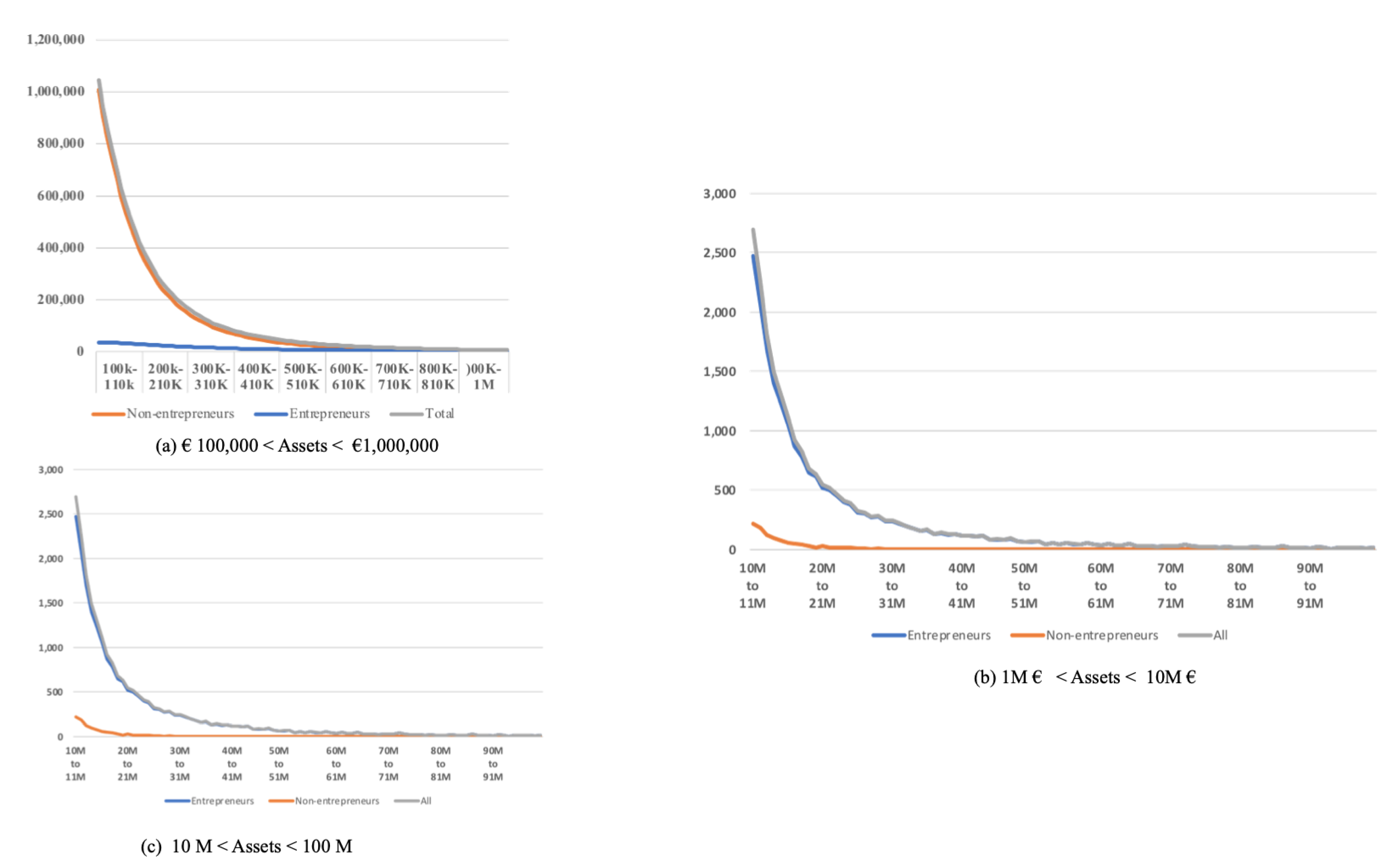
3.4.2. Definition of Subpopulations
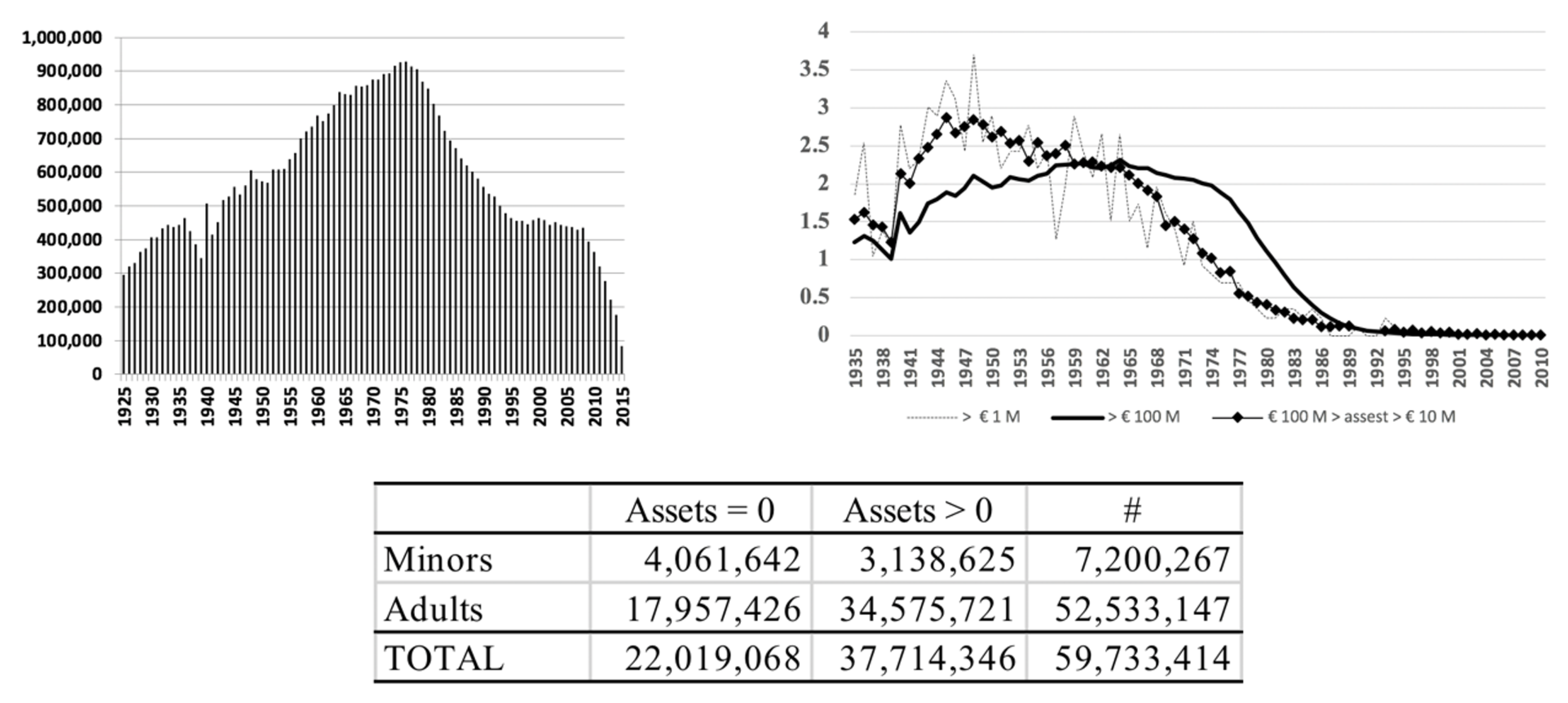
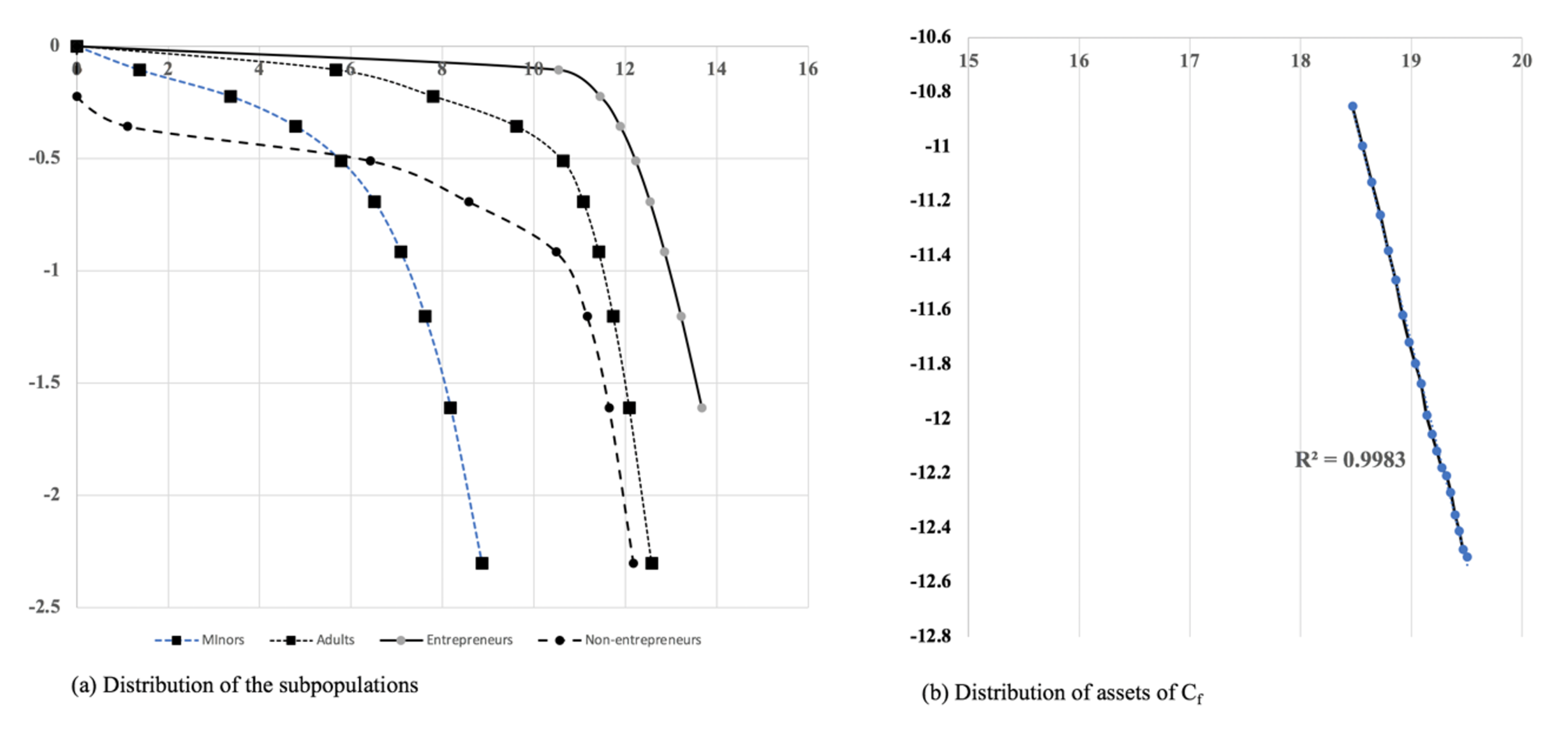
- Taxpayers without assets (). Minors, net debtors, non-resident workers who receive income or subsidies, but do not have assets to their name. Taxpayers with assets () contains the following subgroups.
- Passive taxpayers (). With assets received by donation or inheritance (minors) and attributed to them by third parties (their parents or financial institutions).
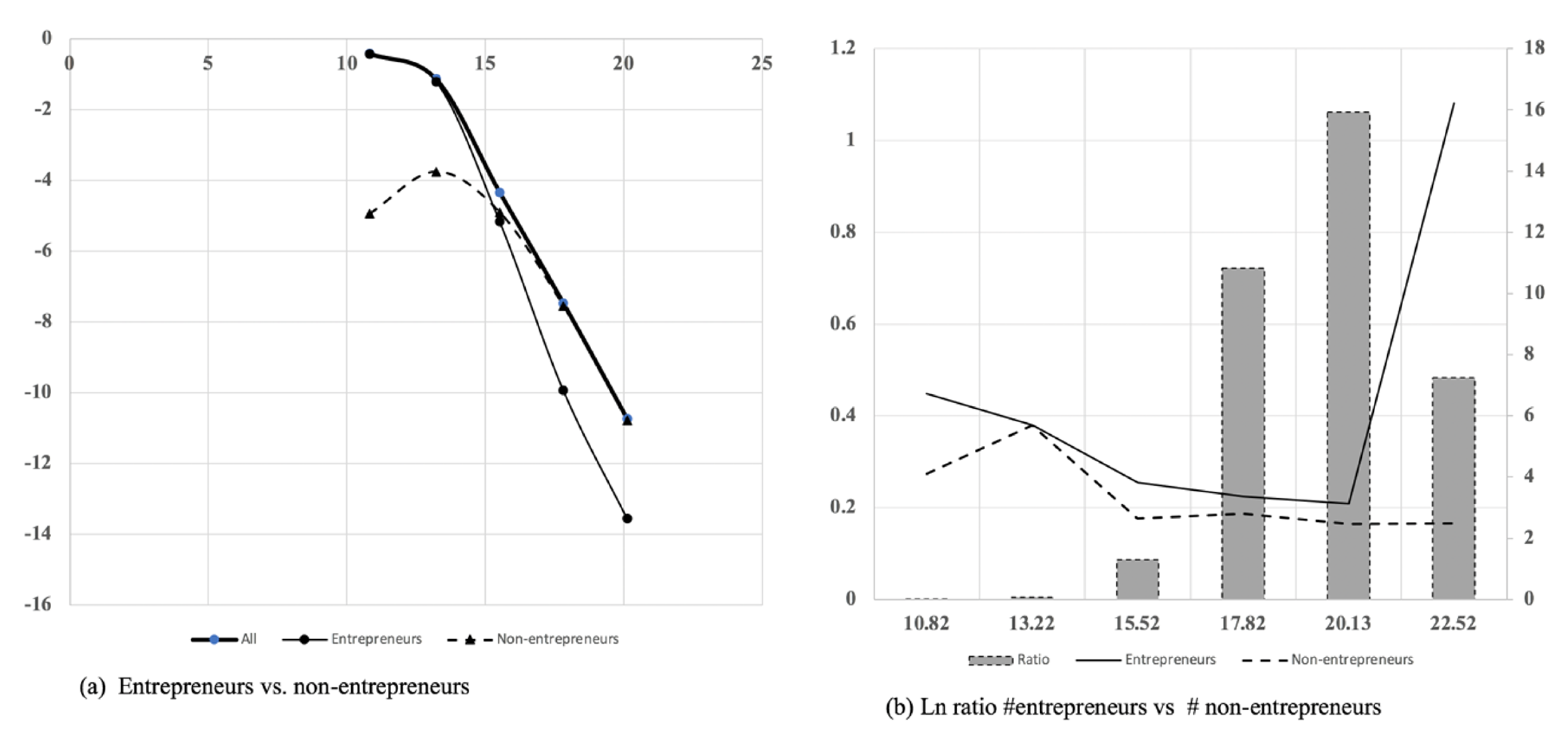
- Non-entrepreneurs (). Salary earners and professionals whose main income is a salary. They do not hold shares in non-listed companies. The wealth generation process is governed by the accumulation of savings.
- Entrepreneurs (). Owners or shareholders in unlisted companies. They are characterized by owning assets, shares in listed companies or participations in companies through other companies. The wealth generation process is a combination of the accumulation characteristic of savings (direct assets) and multiplicative effects (indirect assets), mediated in this case by random a variable (success of the non-listed companies) in a process that can be modelled based on Gibrat’s ideas.
- Large fortunes () are, in some cases, exceptionally successful entrepreneurs but more often holders of large family fortunes. The wealth accumulation process is governed by other rules and is affected by inheritances and marriages.
3.4.3. Distribution of the Subpopulations
3.5. Analysis of the Components of Wealth
- The growing importance of indirect assets (shares in non-listed companies) as we move up from the bottom interval (9.25%) to large fortunes (79.44%), where it far outweighs total financial assets (19.83%) (including shareholdings in IBEX-listed companies).
- The importance of the value of immovable property in the analysis. The share of real estate assets (first and second residences) that decreases with wealth. It represents 73.15% of the wealth of the poorest and accounts for an almost negligible fraction (0.50%) of large fortunes.
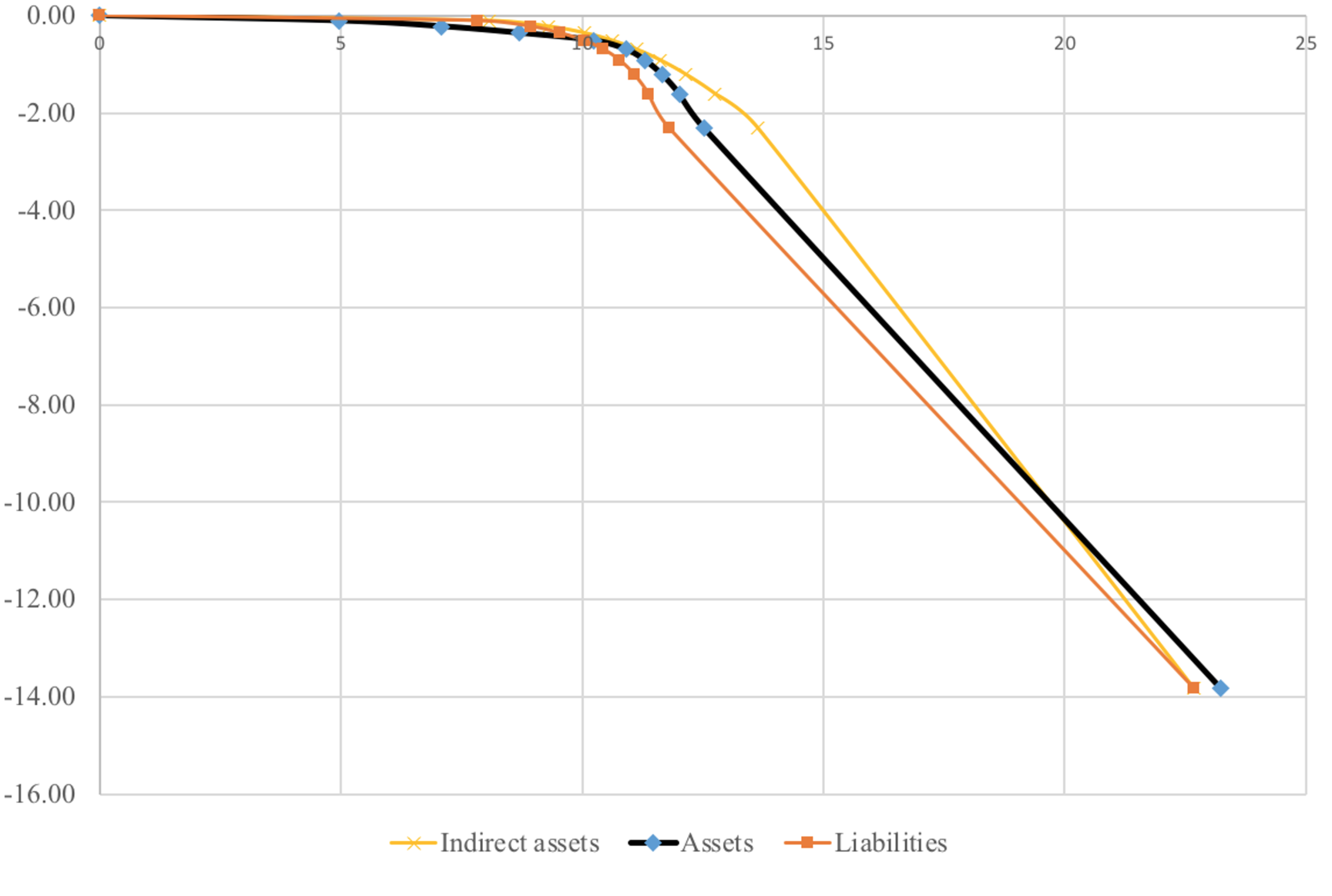
- Liabilities and indirect assets play an extremely important role in conducting a correct analysis. If the variable used does not take liabilities into account, the poor appear to be richer (inequality is attenuated). If indirect assets are not counted, the richest appear to be poorer than they really are.
3.6. Characterization of the Nature of the Underlying Processes
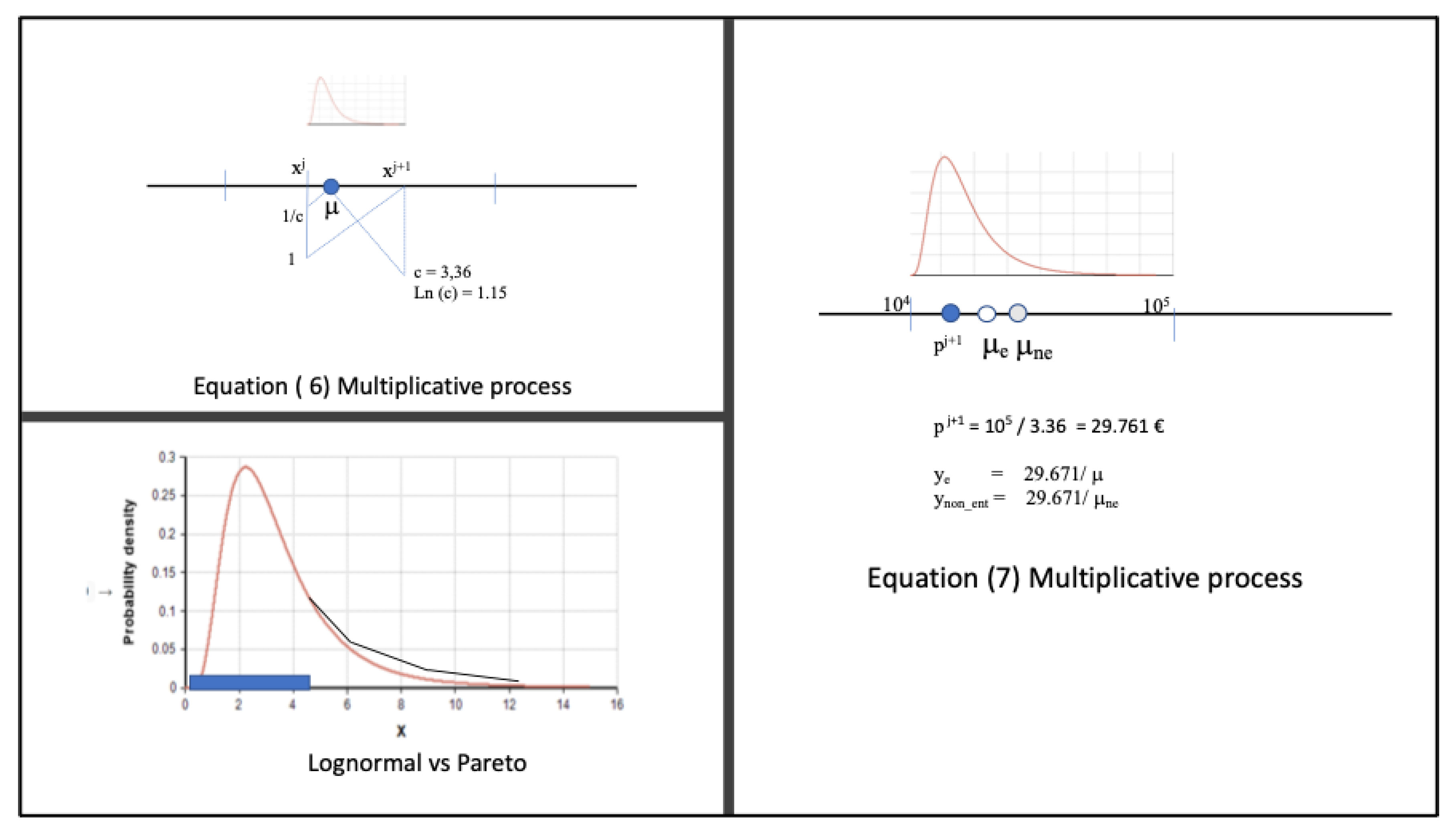
Generation of Additive and Multiplicative Effects
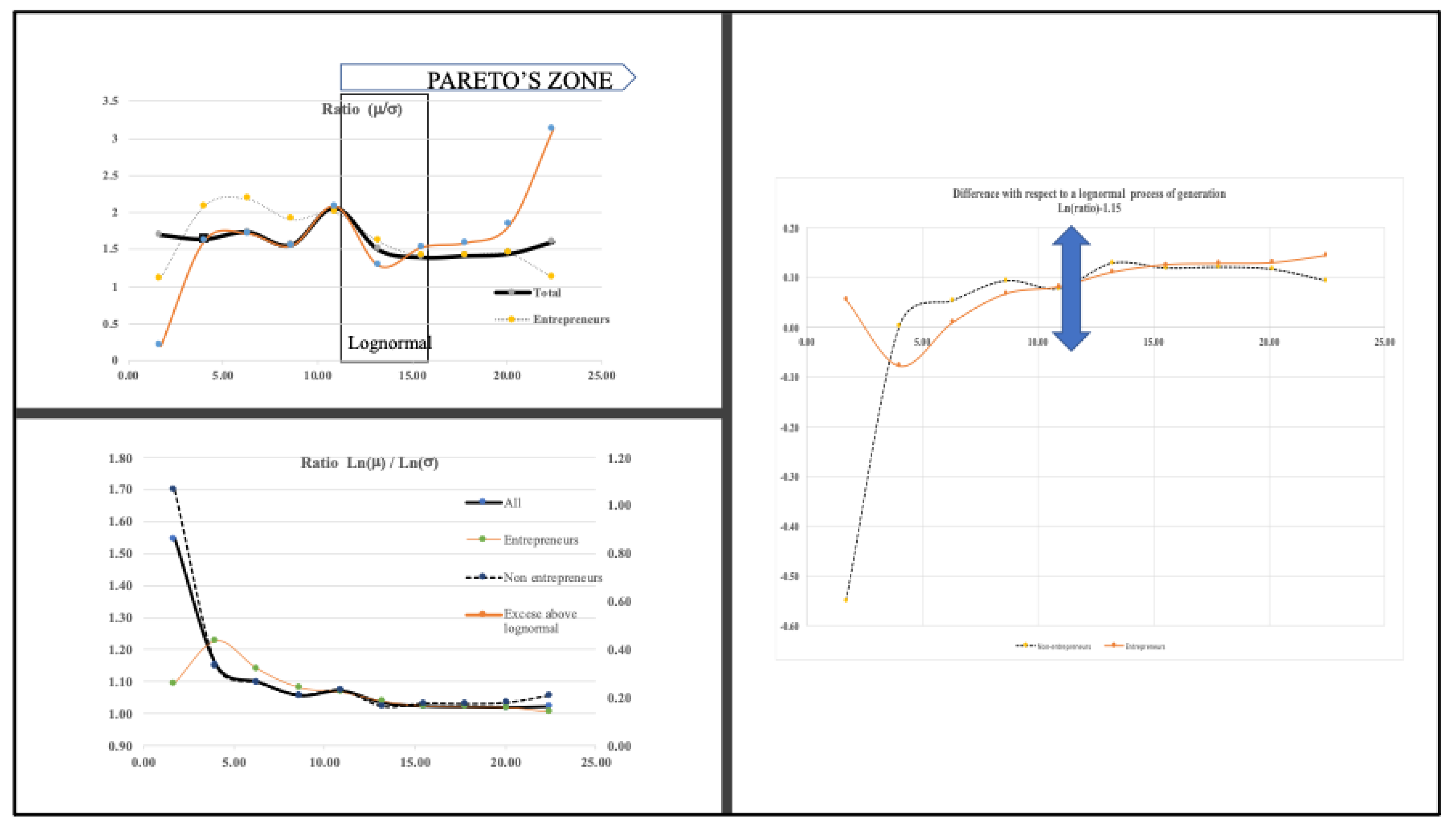
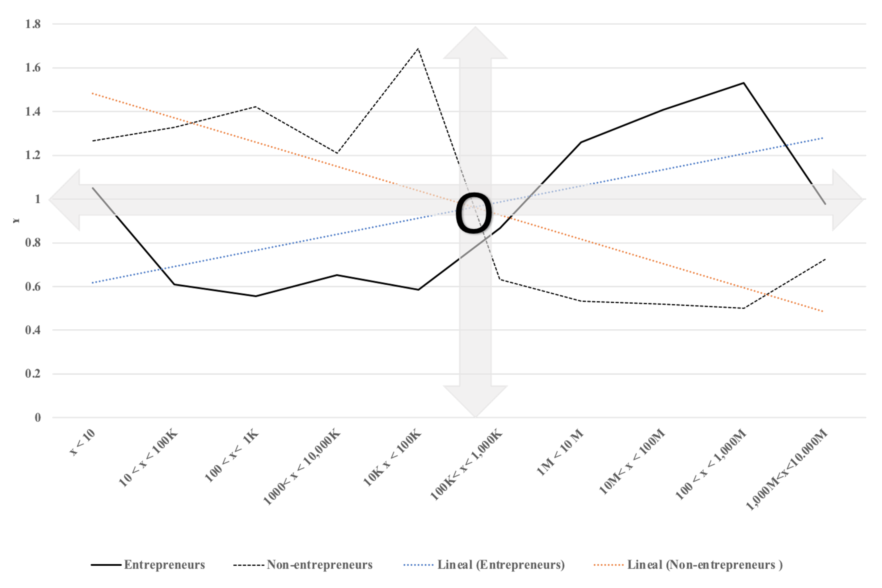
- In each interval , by construction, . For all the intervals, , that is, .
- If the underlying process is multiplicative, with the proposed intervals , it holds that there is a point , in the intervaland, therefore,If we compare the real value for both subpopulations, we would observe any difference with respect to the situation where the accumulative effect holds. We use for this observed value the notation y:and
4. Conclusions
- The best option for analyzing wealth distribution regularities and studying inequality is total assets, including direct and indirect assets, because it uses more relevant data for accurately studying entrepreneur activity. The choice between the two available options of studying positive values or positive and negative values has to be made considering the objectives of the study and the availability of microdata on mortgages.
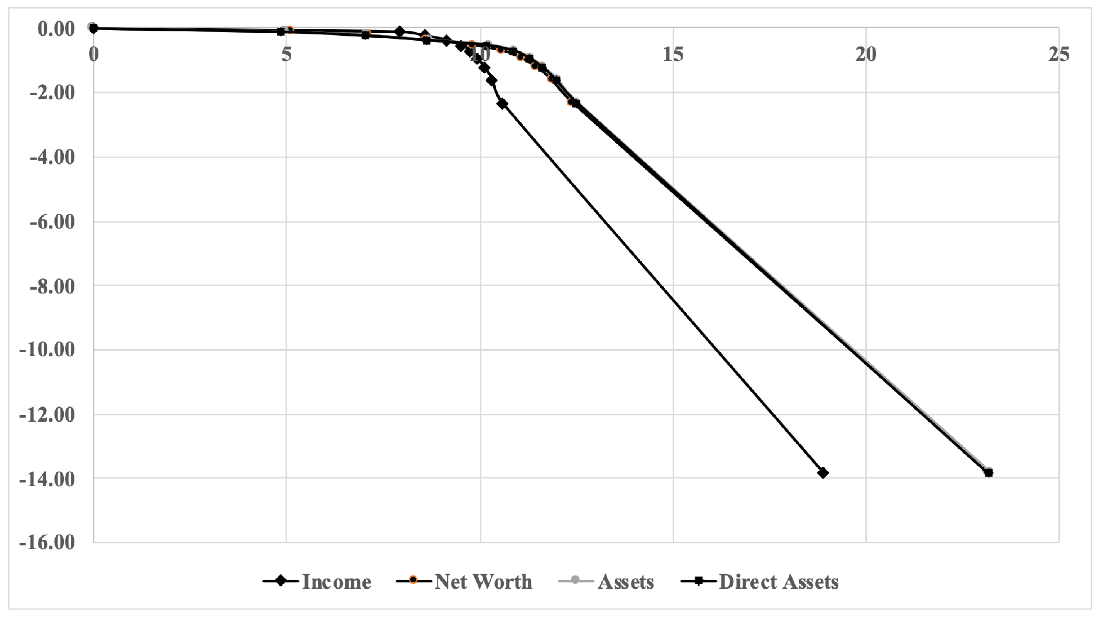
- Analyzing the Spanish population with a wealth distribution in the range , we have found that the best threshold for Pareto analysis is at the point and the best binning is .
- We have identified five subpopulations with the following population shares: (without assets) accounts for 36.86%. Owner of assets is a mixture of four subpopulations, minors, non-entrepreneurs and entrepreneurs and big fortunes.
- We have identified two types of accumulative processes (savings) and (investments), where the region of transition between the processes is . The process of generation of big fortunes is a mixture of both.
- The distribution of the subpopulations with assets in the Pareto zone can be fitted to lognormal curves, but the process of accumulation proposed by Gibrat is clearer for entrepreneurs. Within the population that work for a salary, wealth accumulation is attenuated by the payment of mortgages. Table 4 shows that, on average, 73.15% of the value of assets owned by people that work for a salary takes the form of real estate, that is, their homes, where liabilities (mostly mortgages) account for 63.59% of total assets. Their wealth accumulation is limited by interest payments and is, in some cases, driven by the increase of the property values. There is a huge difference with the average “private” liabilities of entrepreneurs (with total assets ranging from €100 K to €1 M), which are less affected by interest rates.
- The wealth accumulation process is different for large fortunes, where it is relevant the wealth accumulated as shareholdings in non-listed companies.
- Wealth models should consider that: (a) the subpopulation of minors and donees of wealth is distributed so as to reflect the wealth of the donors (and has a lognormal distribution), (b) the population of entrepreneurs (with corporate assets) should be differentiated from the population of employees and professionals (non entrepreneurs), which behave differently, and aggregate behavior with a level of multiplicative symmetry emerges only as a result of the mixture of these two populations.
- We have explained the difference observed in empirical studies with respect to the law of Pareto by the effect in the wealth distribution of two processes of accumulation of wealth, one of them stationary and other characteristics of entrepreneurs that changes within each society with different uses of technology and with the growing importance of financial activities.
Author Contributions
Funding
Institutional Review Board Statement
Informed Consent Statement
Acknowledgments
Conflicts of Interest
References
- Chandra Dash, K. The Story of Econophysics; Cambridge Scholar Publishing: Cambridge, UK, 2019. [Google Scholar]
- Jovanovic, F.; Schinckus, C. The History of Econophysics Emergence: A new Approach in Modern Financial Theory. Hist. Political Econ. 2013, 45, 443–474. [Google Scholar] [CrossRef]
- Savoiu, G.; Siman, I. History and Role of Econophysics in Scientific Research, Cap 1 en Econophysics: Background and Applications in Economics. Financ. Sociophys. 2013, 3–16. [Google Scholar] [CrossRef]
- Stanley, H.E. Stanley on Econophysics; Sage Publication: Sauzend Oaks, CA, USA, 2013; Volume 2, pp. 73–78. [Google Scholar]
- Bouchaud, J.P. Econophysics: Still Fringe after 30 Years? Available online: https://arxiv.org/abs/1901.03691v1 (accessed on 8 February 2021).
- Axtell, R. Zipf distribution of US firm sizes. Science 2001, 293, 1818–1820. [Google Scholar] [CrossRef] [PubMed]
- Atkinson, A.B.; Voitchovsky, S. The distribution of top earnings in the UK since the Second World War. Economica 2010, 78, 440–459. [Google Scholar] [CrossRef]
- Rawls, J. A Theory of Justice; Cambridge, M.A., Ed.; Harvard University Press: Cambridge, MA, USA, 1971. [Google Scholar]
- Sen, A. Poverty and Famines; Oxford University Press: New Delhi, India, 1999. [Google Scholar]
- Forbes, K.J. A reassessment of the relationships between inequality and growth. Am. Econ. Rev. 2000, 90, 869–887. [Google Scholar] [CrossRef]
- Piketty, T. 21 Lessons for the 21st Century; Harvard University Press: Cambridge, MA, USA, 2013. [Google Scholar]
- Mantegna, R.N.; Stanley, H.E. 21 Lessons for the 21st Century; Spiegel & Grau: New York, NY, USA, 2018. [Google Scholar]
- Mantegna, R.N.; Stanley, H.E. An introduction to Econophysics: Correlations and Complexity Finance; Cambridge University Press: Cambridge, UK, 2001. [Google Scholar]
- Chatterjee, A.; Yarlagadda, S.; Chakrabarti, B.K. (Eds.) Econophysics of Wealth Distributions; Springer: Milan, Italy, 2005. [Google Scholar]
- Champernowe, D.G. A model of income distribution. Science 1953, 63, 318–351. [Google Scholar]
- Gibrat, R. Les Inegalités Economiques; Librairie du Recueil. Sirey: Paris, France, 1931. [Google Scholar]
- Santarelli, E.; Klomp, L.; Thurick, R. Gibrat’s Law: An overview of the empiric literature. In International Studies in Entreprenership; Springer: Berlin/Heidelberg, Germany, 2006; Volume 12, pp. 1–73. [Google Scholar]
- Chakrabarti, B.; Chakraborti, A.; Chakrabarty, S.; Chaterjee, A. Econophysics of Income and Wealth Distribution; U.K. Cambridge University Press: Cambridge, UK, 2013. [Google Scholar]
- Richmond, P.; Hutzler, S.; Coelho, R. A review of empirical studies and Models of Income Distributions in Society. In Econophysics and Sociophysics. Trends and Perspectives; Chakrabarti, B.K., Chakabrorti, A., Chaterjee, A., Eds.; Wiley-VCH: Berlin, Germany, 2016. [Google Scholar]
- Atkinson, A.B. The distribution of top incomes in the United Kingdom 1908–2000. In Top Incomes over the 20th Century; Atkinson, A.B., Piketty, T., Eds.; Oxford University Press: Oxford, UK, 2007. [Google Scholar]
- Yakovenko, V.M.; Rosser, J.B. Colloquium: Statistical mechanics of money wealth and income. Econ. J. 2013, 81, 703–725. [Google Scholar] [CrossRef]
- Aoyama, H.; Souma, W.; Nagahara, Y.; Okazaki, M.P.; Takayasu, H.; Takayasu, M. Pareto’s law for income of individuals and debt of bankrupt companies. Fractals 2000, 8, 293–300. [Google Scholar] [CrossRef]
- Aoyama, H.; Souma, W.; Fujiwara, Y. Growth and fluctuations of personal and company’s income. Physica A 2003, 324, 352–358. [Google Scholar] [CrossRef]
- Aoyama, H.; Fujiwara, Y.; Fujiwara, Y. Econophysics and Companies: Statistical Life and Death in Complex Business Networks; Cambridge University Press: New York, NY, USA, 2011. [Google Scholar]
- Shirras, F. The Pareto Law and the Distribution of Income. Econ. J. 1935, 45, 663–681. [Google Scholar] [CrossRef]
- Atkinson, A.B. Pareto and the upper tail of the income distribution in the UK: 1799 to the present. Econ. Spec. Issue Inequality 2017, 84, 129–343. [Google Scholar] [CrossRef]
- Benhabib, J.; Bisin, A. Skewed Wealth Distributions: Theory and Empirics; NBER Working Paper 21924; National Bureau of Economic Research: Cambridge, MA, USA, 2016. [Google Scholar]
- Kleiber, C. Dagum vs. Singh-Maddala income distributions. Econ. Lett. 1996, 53, 265–268. [Google Scholar] [CrossRef]
- Bandourian, R.; McDonald, J.B.; Turkey, R.S. A comparison of parametric models of income distribution across countries and overtime. Estadística 2003, 55, 135–152. [Google Scholar]
- Montroll, E.W.; Schelesinger, M.F. On 1/f noise and other distributions with long tails. Proc. Natl. Acad. Sci. USA 1982, 79, 3380–3383. [Google Scholar] [CrossRef]
- Hogg, R.V.; Mckean, J.W.; Craig, A.T. Introduction to Mathematical Statistics; Pearson Education: Delhi, India, 2007. [Google Scholar]
- Chatterjee, A.; Chakrabarti, B.K. Kinetic exchange models for income and wealth distributions. Eur. Phys. J. B 2006, 60, 135–149. [Google Scholar] [CrossRef]
- Cowell, A.; Flachaire, E. Statistical Methods for Distributional Analysis. In Handbook of Income Distribution; Elsevier: Amsterdam, The Netherlands, 2015. [Google Scholar]
- Chotikapanich, D.; Griffiths, W. Estimating income distributions using a mixture of gamma densities. In Modelling Income Distributions and Lorenz Curves; Chotikapanich, D., Ed.; Springer: New York, NY, USA, 2008; Chapter 16; pp. 285–302. [Google Scholar]
- Pittau, M.G.; Zelli, R. Empirical evidence of income dynamics across EU regions. Italian evidence in the 1990s from kernel density estimates. Empir. Econom. 2006, 29, 415–430. [Google Scholar] [CrossRef]
- AEAT 2020. Available online: www.aeat.es (accessed on 8 February 2021).
- González, I.; Mateos, A. La distribución de la riqueza. Pareo deconstruido, Gibrat reconstruido. Rev. Econ. Apl. Número Extraordin. Econophys. 2019, 37, 22–40. [Google Scholar]
- Kleiber, C.; Kotz, S. Statistical Size Distributions in Economics and Actuarial Sciences; John Willey and Sons: Hoboken, NJ, USA, 2003. [Google Scholar]
- Mandelbrot, B.B. The Pareto Levy law and the distribution of income. Int. Econ. Rev. 1960, 1, 79–106. [Google Scholar] [CrossRef]
- Arnold, B.C. Pareto Distributions, 2nd ed.; CRC Press, Taylor y Francis Group: Boca Raton, FL, USA, 2015. [Google Scholar]
- Richmond, P.; Solomon, S. Stable power laws in variable economics; Lotka-Volterra implies Pareto-Zipf. Eur. Phys. J. B 2002, 27, 257–261. [Google Scholar] [CrossRef]
- Limpert, E.; Stahel, W.A.; Abbt, M. Log-normal Distributions across the Sciences: Keys and Clues. BioScience 2001, 5, 341–352. [Google Scholar] [CrossRef]
- Koch, A.L. The logarithm in biology. I. Mechanisms generating the log-normal distribution exactly. J. Theor. Biol. 1966, 23, 276–290. [Google Scholar] [CrossRef]
- Koch, A.L. The logarithm in biology. II. Mechanisms generating the log-normal distribution exactly. J. Theor. Biol. 1966, 23, 251–268. [Google Scholar] [CrossRef]
- Coelho, R.; Neda, Z.; Ramasco, J.; Santos, A. A family-network model for wealth distribution in societies. Physica A 2005, 353, 515–528. [Google Scholar] [CrossRef]
- Gabaix, X. Power laws in economics and finance. Annu. Rev. Econ. 2009, 1, 255–294. [Google Scholar] [CrossRef]
- Montebruno, P.; Bennet, R.J.; Van Lieshout, C.; Smith, H. A tale of two tails: Do power Law and Lognormal models fit firm size distribution in the mid-Victorian Era? Physica A 2019, 523, 858–865. [Google Scholar] [CrossRef]
- Solomon, S.; Richmond, P. Power laws of wealth, market order volumes and market returns. Physica A 2001, 299, 188. [Google Scholar] [CrossRef]
- Pareto, V. Cours d’Economie Politique; Trad. “Manual of Political Economy”; Macmillan: Paris, France; London, UK, 1897; Volume 2. [Google Scholar]
- Dempster, A.P.; Laird, N.M.; Rubin, D.B. Maximum Likelihood from Incomplete Data via the EM Algorithm. J. R. Stat. Soc. Ser. 1977, 39, 1–38. [Google Scholar]
- Brindusa, A.; Basso, H.; Bover, O.; Casado, J.M.; Hospido, L.; Izquierdo, M.; Kataryniu, I.; Lacuesta, A.; Montero, J.M.; Vozmediano, E. La desigualdad de la renta el consumo y la riqueza en España. Doc. Ocas. Banco Espa. 2018, 6, 1–49. [Google Scholar]
- Chescher, A.; Schluter, C. Measurement error and inequality measurement. Rev. Econ. Stud. 2002, 69, 357–378. [Google Scholar] [CrossRef]
- Atkinson, A.B.; Piketty, T.; Saez, E. Top incomes in the long run oftheirtory. J. Econ. Lit. 2011, 49, 3–71. [Google Scholar] [CrossRef]
- Silverman, B.W. Density Estimation for Statistics and Data Analysis; Chapman & Hall/CRC: London, UK, 1986. [Google Scholar]
- Garcia Docampo, M. Medición del análisis de las desigualdades en la distribución de la renta. Empiria. Rev. Metodol. Las Cienc. Soc. 2000, 3, 73–99. [Google Scholar]
- Gut, C.; Limpert, E.; Hinterberger, H. A Computer Simulation on the Web to Visualize the Genesis of Normal and Log-Normal Distributions. 2000. Available online: http://stat.ethz.ch/vis/log-normal (accessed on 8 February 2021).



| INCOME | NET WORTH | ASSETS > 0 | ||||
|---|---|---|---|---|---|---|
| >0 | >0 | <0 | Total | Direct | Indirect | |
| ∑ (M€) | 442,810 | 4,228,499 | −123,893 | 5,504,770 | 4,372,866 | 1,131,697 |
| 20,593 | 114,205 | −27,335 | 145,959 | 115,974 | 21,936 | |
| # | 21,472,065 | 37,025,366 | 4,532,469 | 37,714,346 | 37,714,346 | 1,458,186 |
| 59,448 | 5,142,106 | 202.669 | 5,423,997 | 4,216,853 | 3,321,528 | |
| D1 | 2806 | 165 | −65,663 | 143 | 128 | 0 |
| D2 | 5267 | 1258 | −41,439 | 1202 | 1123 | 0 |
| D3 | 9326 | 5417 | −27,605 | 5996 | 5490 | 0 |
| D4 | 13,632 | 18,652 | −18,286 | 27,783 | 26,145 | 0 |
| Me | 16,655 | 39,897 | −11,892 | 54,621 | 53,137 | 0 |
| D6 | 20,088 | 64,136 | −7558 | 81,058 | 79,063 | 0 |
| D7 | 24,336 | 95,216 | −4393 | 114,745 | 111,579 | 0 |
| D8 | 30,210 | 142,423 | −1820 | 165,736 | 159,887 | 0 |
| D9 | 38,428 | 240,632 | −480 | 273,795 | 270,312 | 0 |
| Var. | 2015 | 2016 | 2017 | 2018 | 2016/2015 | 2017/2015 | 2018/2015 |
|---|---|---|---|---|---|---|---|
| ∑ | 5,504,811 | 6,522,811 | 5,925,214 | 6,297,723 | 118.49 | 107.64 | 114.40 |
| 149,959 | 168,858 | 156,417 | 1190,390 | 115.69 | 107.17 | 130.44 | |
| 4,916,808 | 126,005 | 127,548 | 3,972,678 | 2.56 | 2.59 | 80.80 | |
| # | 37,714,346 | 38,806,625 | 37,880,766 | 38,072,958 | 102.90 | 100.44 | 100.95 |
| Interval € | # | Interval | # | Interval | # | Interval | # |
|---|---|---|---|---|---|---|---|
| 1 to 10 | 1,845,563 | <100 | 3,522,730 | <1 K | 7,512,309 | <10 K | 13,411,653 |
| 10 to 20 | 419,723 | 100 to 200 | 858,755 | 1 K to 2 K | 1,791,396 | 10 K to 20 K | 1,520,055 |
| 20 to 30 | 264,339 | 200 to 300 | 606,925 | 2 K to 3 K | 1,035,198 | 20 K to 30 K | 1,447,770 |
| 30 to 40 | 205,114 | 300 to 400 | 508,197 | 3 K to 4 K | 744,920 | 30 K to 40 K | 1,520,055 |
| 40 to 50 | 161,698 | 400 to 500 | 430,310 | 4 K to 5 K | 564,586 | 40 K to 50 K | 1,614,721 |
| 50 to 60 | 186,280 | 500 to 600 | 390,268 | 5 K to 6 K | 465,260 | 50 K to 60 K | 1,639,613 |
| 60 to 70 | 133,745 | 600 to 700 | 347,597 | 6 K to 7 K | 397,574 | 60 K to 70 K | 1,591,818 |
| 70 to 80 | 113,784 | 700 to 800 | 309,361 | 7 K to 8 K | 336,237 | 70 K to 80 K | 1,483,085 |
| 80 to 90 | 104,315 | 800 to 900 | 281,055 | 8 K to 9 K | 300,479 | 80 K to 90 K | 1,353,336 |
| 90 to100 | 88,169 | 900 to 1K | 257,111 | 9 K to 10 K | 263,694 | 90 K to 100 K | 1,231,181 |
| ∑ | 3,522,730 | 7,512,309 | 13,411,653 | 27,146,544 |
| % WITH RESPECT TO TOTAL ASSETS | ||||||
|---|---|---|---|---|---|---|
| Interval | # | Liabilities | Indirect Assets | Real Estate | Current Accounts | FF.AA |
| Less 100 K | 29,965,372 | 63.59 | 9.25 | 73.15 | 14.03 | 3.57 |
| 100 K to 1 M | 9,629,289 | 11.01 | 8.24 | 70.35 | 15.27 | 6.14 |
| 1 M to 10 M | 364,357 | 17.63 | 40.23 | 37.59 | 7.19 | 14.99 |
| 10 M to100 M | 14,326 | 23.05 | 69.62 | 9.09 | 3.11 | 18.18 |
| 100 M to 1000 M | 471 | 25.45 | 79.47 | 2.03 | 1.74 | 16.76 |
| >1000 M | 19 | 26.43 | 79.44 | 0.23 | 0.50 | 19.83 |
| # | Range | ||||
|---|---|---|---|---|---|
| Total Population | 59,733,414 | [0, 10,000 M] | |||
| WITHOUT ASSETS | 22,019,068 | 0 | 0 | ||
| Minors without assets | 3,128,625 | ||||
| Adults without assets | 18,890,443 | [0, 10,000 M] | |||
| ASSET OWNERS < 0 | 4,532,569 | ||||
| ASSET OWNERS | 37,714,346 | [0, a ∗ 10,000 M] | |||
| Minors with assets | 4,072,002 | [0;130 M] | 5 | 165 | |
| Adults with assets | 34,585,721 | [[0, a ∗ 10,000 M] | 159 | 4,318,838 | |
| Non-entrepreneurs | 35,256,160 | [0, 10,000 M] | 98,974 | 217 | |
| Entrepreneurs | 1,458,186 | [0;100 M] | 890 | 3,031,214 | |
| Big fortunes (>100 M) | 917 | [100 M, a ∗ 10,000 M] | 318,213,094 | 787,168,132 | |
| Entrepreneurs | 863 | [100 M, a ∗ 10,000 M] | 314,059,377 | 785,624,254 | |
| Other cases | 44 | [100 M, a ∗ 10,000 M] | 512,925,903 | 857,383,064 |
| ENTREPRENEURS | NON-ENTREPRENURS | E | N.E | E | N.E | |||||
|---|---|---|---|---|---|---|---|---|---|---|
| Ln() | Ln() | Exc. | Exc. | |||||||
| 0–1 | 3.34 | 3.01 | 1.11 | 0.02 | 0.10 | 0.20 | 1.09 | 1.70 | 0.06 | −0.55 |
| 1–2 | 52 | 25 | 2.08 | 42 | 26 | 1.62 | 1.23 | 1.15 | −0.08 | 0.00 |
| 2–3 | 569 | 261 | 2.18 | 450 | 263 | 1.71 | 1.14 | 1.10 | 0.01 | 0.05 |
| 3–4 | 4840 | 2543 | 1.90 | 3830 | 2471 | 1.55 | 1.08 | 1.06 | 0.07 | 0.09 |
| 4–5 | 54,091 | 27,005 | 2.00 | 53,382 | 25,653 | 2.08 | 1.07 | 1.07 | 0.08 | 0.08 |
| 5–6 | 364,262 | 225,982 | 1.61 | 199,751 | 156,081 | 1.28 | 1.04 | 1.02 | 0.11 | 0.13 |
| 6–7 | 2,510,687 | 1,780,143 | 1.41 | 1,686,501 | 1,100,573 | 1.53 | 1.02 | 1.03 | 0.13 | 0.12 |
| 7–8 | 22,482,106 | 15,811,009 | 1.42 | 16,394,325 | 10,320,486 | 1.59 | 1.02 | 1.03 | 0.13 | 0.12 |
| 8–9 | 206,604,515 | 143,069,745 | 1.44 | 158,398,773 | 86,480,258 | 1.83 | 1.02 | 1.03 | 0.13 | 0.12 |
| 9–10 | 3,233,259,800 | 2,871,975,594 | 1.13 | 2,286,954,185 | 732,488,355 | 3.12 | 1.01 | 1.06 | 0.14 | 0.09 |
| 100 K < Actives < 1 M | 1 M < Actives < 100 M | 100 M < Actives < 500 M | 1500 M < Actives < 15 KM | |||||
|---|---|---|---|---|---|---|---|---|
| Year | Entrep. | N-Entrep. | Entrep. | N-Entrep. | Entrep. | N-Entrep. | Entrep. | N-Entrep. |
| 2015 | 1,143,143 | 11,151,678 | 324,620 | 193,889 | 763 | 15 | 82 | 3 |
| 2016 | 1,183,178 | 11,330,440 | 333,804 | 206,028 | 796 | 19 | 92 | 1 |
| 2017 | 1,176,698 | 11,970,874 | 363,025 | 276,286 | 822 | 22 | 102 | 2 |
| 2018 | 1,192,844 | 11,225,120 | 375,442 | 281,007 | 877 | 20 | 99 | 10 |
| Interval | (Entrepreneurs) | (Non-Ent.) | ||||
|---|---|---|---|---|---|---|
| 0–1 | 0.5 | 3.16 | 3 | 1.05 | 4 | 1.26 |
| 1–2 | 1.5 | 31.62 | 52 | 0.61 | 42 | 1.33 |
| 2–3 | 2.5 | 316 | 569 | 0.56 | 450 | 1.42 |
| 3–4 | 3.5 | 3162 | 4840 | 0.65 | 3830 | 1.21 |
| 4–5 | 4.5 | 31.623 | 54,091 | 0.58 | 53,382 | 1.69 |
| 5–6 | 5.5 | 316,228 | 364,262 | 0.87 | 199,751 | 0.63 |
| 6–7 | 6.5 | 3,162,278 | 22,482,106 | 1.26 | 1,686,501 | 0.53 |
| 7–8 | 7.5 | 31,622,777 | 22,482,106 | 1.41 | 16,394,325 | 0.52 |
| 8–9 | 8.5 | 316,227,766 | 206,604,515 | 1.53 | 158,398,773 | 0.50 |
| 9–10 | 9.5 | 3,162,277,660 | 3,233,249,800 | 0.98 | 2,286,954,185 | 0.72 |
Publisher’s Note: MDPI stays neutral with regard to jurisdictional claims in published maps and institutional affiliations. |
© 2021 by the authors. Licensee MDPI, Basel, Switzerland. This article is an open access article distributed under the terms and conditions of the Creative Commons Attribution (CC BY) license (http://creativecommons.org/licenses/by/4.0/).
Share and Cite
González García, I.; Mateos Caballero, A. Models of Wealth and Inequality Using Fiscal Microdata: Distribution in Spain from 2015 to 2020. Mathematics 2021, 9, 377. https://doi.org/10.3390/math9040377
González García I, Mateos Caballero A. Models of Wealth and Inequality Using Fiscal Microdata: Distribution in Spain from 2015 to 2020. Mathematics. 2021; 9(4):377. https://doi.org/10.3390/math9040377
Chicago/Turabian StyleGonzález García, Ignacio, and Alfonso Mateos Caballero. 2021. "Models of Wealth and Inequality Using Fiscal Microdata: Distribution in Spain from 2015 to 2020" Mathematics 9, no. 4: 377. https://doi.org/10.3390/math9040377
APA StyleGonzález García, I., & Mateos Caballero, A. (2021). Models of Wealth and Inequality Using Fiscal Microdata: Distribution in Spain from 2015 to 2020. Mathematics, 9(4), 377. https://doi.org/10.3390/math9040377


