Article

Nonlocal Reaction–Diffusion Models of Heterogeneous Wealth Distribution

by
Malay Banerjee
1,
Sergei V. Petrovskii
2 and
Vitaly Volpert
3,4,5,*
1
Department of Mathematics & Statistics, IIT Kanpur, Kanpur 208016, India
2
School of Mathematics & Actuarial Science, University of Leicester, Leicester LE1 7RH, UK
3
Institut Camille Jordan, UMR 5208 CNRS, University Lyon 1, 69622 Villeurbanne, France
4
INRIA Team Dracula, INRIA Lyon La Doua, 69603 Villeurbanne, France
5
Peoples’ Friendship University of Russia (RUDN University), 6 Miklukho-Maklaya St, 117198 Moscow, Russia
*
Author to whom correspondence should be addressed.
Mathematics 2021, 9(4), 351; https://doi.org/10.3390/math9040351
Submission received: 5 January 2021 / Revised: 27 January 2021 / Accepted: 2 February 2021 / Published: 10 February 2021

Abstract

:
Dynamics of human populations can be affected by various socio-economic factors through their influence on the natality and mortality rates, and on the migration intensity and directions. In this work we study an economic–demographic model which takes into account the dependence of the wealth production rate on the available resources. In the case of nonlocal consumption of resources, the homogeneous-in-space wealth–population distribution is replaced by a periodic-in-space distribution for which the total wealth increases. For the global consumption of resources, if the wealth redistribution is small enough, then the homogeneous distribution is replaced by a heterogeneous one with a single wealth accumulation center. Thus, economic and demographic characteristics of nonlocal and global economies can be quite different in comparison with the local economy.

1. Introduction

Distribution of wealth is a factor that defines social justice and, as such, is believed to determine the stability of society [1]. It also affects the rate of economic development; in particular, it is thought that a certain degree of inequality is necessary to stimulate the economic growth [2,3], although the issue remains controversial [4]. Patterns of wealth distribution have been attracting keen scientific attention ever since the seminal work by Pareto [5,6]. Traditional approach to this matter is based on data collection (e.g., through the tax office) and their statistical analysis, which allows one to reveal the trends such as, for instance, an increase or decrease of the inequality [7,8]. Although providing valuable information, this approach alone has a limited power to explain the reasons behind the corresponding social and financial dynamics. Mathematical modelling is increasingly regarded as a powerful research tool across life sciences and social sciences [9,10]. Over the last few decades, along with the research based on analysis of relevant financial, social and political data, there have been growing literature concerned with mathematical modelling of the wealth distribution [11,12,13,14,15,16].
Although there has been some growing interest in spatially explicit models over the last two decades [12,15], most of modelling studies available in the literature are concerned with the distribution of wealth over different social groups in a non-spatial context (e.g., see [16] and the references there), for instance in a particular area or city, or on the nationwide scale, hence largely ignoring the heterogeneity of wealth distribution across space. Meanwhile, such heterogeneity can be remarkable, even within the same country; an example is shown in Figure 1. Interestingly, while on a smaller spatial scale (e.g., down to the county level, see Figure 1, left) the distribution looks random, on a larger spatial scale of individual states level it exhibits features reminiscent of periodicity. One example of an apparently nearly periodic behavior is shown in Figure 1 (right) where small and large values of the Gini coefficient (which quantifies the inequality in the wealth distribution) alternates in the East-West direction.
Although it is not our aim in this paper to compare the modelling results with the data, Figure 1 have been an inspiration for this study, where we endeavor to look for a generic mechanism that may result in a spatially heterogeneous wealth distribution. We mention here that obviously, such heterogeneity can arise for a variety of reason. Heterogeneity of the transportation system, e.g., in the road network is one reason as it may affect the availability of jobs [18]. Arguably, heterogeneity in the distribution of natural resources may have a similar effect. Here we hypothesize that apart from the above and other similar reasons, there may exist a generic dynamical mechanism of wealth distribution that can lead to the formation of a heterogeneous spatial pattern. Mathematically, our model is described by coupled nonlinear partial differential equations of reaction–diffusion type that are extended to take into account the nonlocal nature of some of the processes. Being inspired by the success of similar approaches in describing complex population dynamics systems [19,20,21,22], in this paper we consider a spatially explicit model that links the wealth distribution to the population density.

2. Reaction–Diffusion Model of Population-Wealth Distribution

2.1. Basic Model with Constant Resources

We will describe the dynamics of human populations with a conceptual economic–demographic model suggested in [23,24]. The model quantifies the population density p ( x , t ) and the distribution of wealth u ( x , t ) . It consists of two partial differential equations of reaction–diffusion type:
u t = D u 2 u x 2 + F ( u , p ) ,
p t = D p 2 p x 2 + G ( u , p ) ,
where we neglect a possible effect of cross-diffusion introduced in [23]. The first term in the right-hand side of Equation (2) describes the movement of the population in space considered to be random. The diffusion term in Equation (1) characterizes local wealth redistribution due to the economic activities such as trade and investments, and/or taxes.
The population growth in Equation (2) is described by the function
G ( u , p ) = α p ( K ( u ) p ) σ ( u ) p
with the logistic growth characterized by the fertility rate α and the carrying capacity K ( u ) . The second term describes mortality of the population with rate σ ( u ) . Both the carrying capacity and the mortality rates depend on the wealth. For the mortality rate, we consider it to be a monotonously decreasing function of wealth. It takes into account the general observation that on average, the mortality rate is lower for wealthier people due to access to better health services and healthier lifestyle [25]. More specifically, we consider the dependence:
σ ( u ) = σ 0 σ 1 u 1 + u ,
where σ 0 and σ 1 are positive parameters.
In order characterize the function K ( u ) , we note that it describes an equilibrium population density determined by the availability of resources [26]. When the resources decrease, the carrying capacity decreases too and may ultimately go to zero when the resources are completely depleted and hence the environment is not capable any more to support the population. Therefore, for small u, K ( u ) is an increasing function. However, when the resource (wealth) becomes abundant, K ( u ) can lose its monotonicity. Please note that in our formulation of the logistic growth, the linear per capita fertility rate is α K ( u ) . Thus, changes in the carrying capacity reflect the changes in the fertility rate. It has been observed that that there is a certain wealth-dependent difference between low-income and high-income society groups, so that wealthier people, on average, have less children [27]. Accordingly, we consider the carrying capacity K ( u ) to be an increasing function of wealth for small u but decreasing function for large u. Specifically, we consider the carrying capacity in the following form:
K ( u ) = a 2 u u 2 + c 2 2 + ψ 0 ,
where a 2 and c 2 are some positive parameters, and ψ 0 is a part of carrying capacity independent of wealth.
Reaction term in Equation (1) is considered in the following form:
F ( u , p ) = W ( u , p ) S ( u , p ) ,
where W and S are the rates of the wealth production and consumption, respectively. Wealth production is described by the Cobb-Douglas dependence:
W = b H ν Q β M γ ,
where H is the labor, Q is the capital, and M available resources, parameter b characterizes the level of technology, ν , β , and γ are positive constants [28,29]. Please note that in our model we consider “resources” in a broad sense, as any element that is essentially involved in the production of wealth and facilitates the production. Therefore, M quantifies not only the availability of natural resources, both renewable and non-renewable, but also technological resources such as qualification and skills of the labor force (and hence the availability of relevant training and education), the existence and availability of relevant software, etc. We further assume that capital Q is a function of wealth, Q = h ( u ) , and labor is a function of the population density, H = g ( p ) . Then
W ( u , p ) = h ( u ) g ( p ) M
(where we consider ν = β = γ = 1 for the sake of simplicity). We assume that h ( u ) and g ( p ) are increasing functions of their variables with saturation. We choose them in the generic form:
h ( u ) = a 1 u u + c 1 , g ( p ) = p p + c 2 ,
where a 1 , c 1 and c 2 are some positive parameters.
We assume that the wealth consumption S is determined by the depreciation (in particular in case of buildings, machinery, etc.) and due to the consumption of the goods and products by the people. Depreciation is considered to be a linear process with a constant rate a. The rate of the individual (per capita) consumption, c, can be described by the Keynes linear consumption function, c = r + s y , where y is the per capita income, r and s are some positive coefficients. Assuming additionally that average income is proportional to the wealth, we arrive at the following expression: S ( u , p ) = a u + ( r + s u ) p . Altogether, we obtain the following expressions for the functions F and G:
F ( u , p ) = a 1 u p ( u + c 1 ) ( p + c 2 ) M ( a u + ( s + r u ) p ) ,
G ( u , p ) = α p a 2 u u 2 + c 2 2 + ψ 0 p σ 0 σ 1 u 1 + u p .
Please note that in the corresponding non-spatial system with the reaction terms defined as above, Ω = { p > 0 , < u < } is an invariant domain but R + 2 is not. Negative values of u are interpreted as debt; for example, and further discussion see [24].
In the next section we will discuss how to determine available resources M in the wealth production function.

2.2. Variable Resources

System of Equations (1) and (2) with functions F ( u , p ) , G ( u , p ) defined above was introduced in [24] under the assumptions that available resources M are constant. In this work we will study the case of variable resources, and we discuss in this section their dependence on wealth taking into account that consumption of resources can be local or nonlocal:
  • Local dependence on wealth: M 1 ( u ) = ( μ + θ u ) ( 1 k u ) . The first factor ( μ + θ u ) shows that extraction of resources depends on wealth, and the second factor ( 1 k u ) that resources are consumed proportionally to wealth. Here μ , θ , and k are some positive parameters.
  • Nonlocal dependence on wealth: M 2 ( u , J ( u ) ) = ( μ + θ u ) ( 1 k J ( u ) ) , where J ( u ) = ϕ ( x y ) u ( y , t ) d y , where the kernel ϕ ( x y ) shows how the consumption of resources depends on the distance | x y | . The kernel function ϕ ( x ) is even and non-negative. It can take into account the cost of transportation and other factors limiting the usage of distant resources.
  • Global dependence on wealth: M 3 ( u , I ( u ) ) = ( μ + θ u ) ( 1 k I ( u ) ) , where I ( u ) = u ( y , t ) d y . In this case, resources are available independently of their location. In particular, this may be the case of intellectual property, software, and other “immaterial” resources, or the cases where the cost of transportation and other distance-related expenses can be neglected.
Let us note that the form of the function M 1 ( u ) implies that it vanish for u = 1 / k . This means that resources are exhausted for the same level of wealth, which is for the same level of consumption, in spite of the fact that the production of resources increases as a function of wealth. This assumption can be justified if there are several different types of resources such that the production of some of them increases with wealth, while the production of some other remains constant. Hence, there are some limiting resources whose exhaustion occurs for the same level of consumption. For example, agricultural production requires earth and technical equipment. Additional equipment does not increase the level of production if earth is limited, assuming that this equipment does not increase the production per unit area.
In a more general case, we set M 1 ( u ) = ( μ + θ u ) ( 1 + κ u k u ) , where the term 1 + κ u is the exhaustion limit, which now depends on wealth. If κ < k , then this case is reduced to the previous one. The opposite inequality leads the unrealistic situation of the unlimited production and consumption of resources.
In the case of nonlocal consumption of resources, we now have M 2 ( u ) = ( μ + θ u ) ( 1 + κ u k J ( u ) ) . Contrary to the local consumption of resources, the case κ > 0 cannot be reduced to the case κ = 0 , unless it is neglected if κ is small enough. A similar remark concerns the global consumption of resources.

3. Wealth Distribution in Excess of Human Resources

We begin the analysis of system (1) and (2) with a special case where the population grows on a much longer time scale, and hence in the dynamics of wealth the available human resources (quantified by variable p) can be considered to be constant. Correspondingly, we consider the equation
u t = D u 2 u x 2 + F ( u , p ) ,
where
F ( u , p ) = W ( u , p ) S ( u , p ) ,
W ( u , p ) = a 1 u p ( u + c 1 ) ( p + c 2 ) M , S ( u , p ) = a u + ( s + r u ) p ,
and p is assumed to be a positive constant. Assuming that s = 0 and scaling the time and space variables (keeping for them the same notation), we can write Equation (3) in the following form:
u t = D 2 u x 2 + θ u ( b + u ) 1 + k 1 u ( 1 + κ u k 2 H i ) k 3 u ,
where i = 1 , 2 , 3 , the parameters of this equation can be easily expressed through the parameters of Equation (3), and H 1 = u , H 2 = J ( u ) , H 3 = I ( u ) . To reduce the number of parameters and to simplify the calculations, we set in what follows θ = 1 , κ = 0 .
For i = 1 , the nonlinearity
F 1 ( u ) = u ( b + u ) 1 + k 1 u ( 1 k 2 u ) k 3 u
has from one to three non-negative zeros, u = 0 , and up to two positive zeros, u * and u * , u * < u * . They can be found as roots of a second order polynomial. Clearly, F 1 ( u ) < 0 for u > 1 / k 2 . We will denote the largest positive solution u * . It is stable as solution of the equation d u / d t = F 1 ( u ) . If u = 0 is also a stable solution, then there is an additional unstable solution u * . If u = 0 is unstable, then the positive solution u * is unique.
Considered on the whole axis, Equation (4) can have mono-stable or bistable waves with the limits u = 0 and u * at infinity, and a pulse solution. The latter is a stationary solution of this equation with the zero limits at infinity. It exists in the bistable case if and only if 0 u * F 1 ( u ) d u > 0 , and this solution is unstable. These are well-known results [30], and we will not discuss them in detail here.

3.1. Nonlocal Consumption of Resources

In the case of nonlocal consumption of resources, we consider the equation
u t = D 2 u x 2 + F 2 ( u , J ( u ) ) ,
on the whole axis, where
F 2 ( u , J ( u ) ) = f ( u ) ( 1 k 2 J ( u ) ) k 3 u ,
f ( u ) = u ( b + u ) 1 + k 1 u , J ( u ) = ϕ ( x y ) u ( y , t ) d y .
Without loss of generality, we can assume that ϕ ( x y ) d x = ϕ ( x y ) d y = 1 . Then this equation has the same homogeneous-in-space stationary solution u = 0 , u * , u * as Equation (4) in the local case i = 1 .
We will study the stability of the homogeneous-in-space stationary solution u = u * . This solution satisfies the equation
f ( u * ) ( 1 k 2 J ( u * ) ) k 3 u * = 0 , ( J ( u * ) = u * ) .
Consider the operator linearized about this solution:
L v = D v + f ( u * ) ( 1 k 2 u * ) v k 2 f ( u * ) J ( v ) k 3 v .
Taking into account equality (6), we can write it as follows:
L v = D v + a v k 2 f ( u * ) J ( v ) ,
where
a = f ( u * ) f ( u * ) u * ( 1 k 2 u * ) .
Applying the Fourier transform to the equation L v = λ v , we obtain explicit expressions for the eigenvalues:
λ ( ξ ) = D ξ 2 + a k 2 f ( u * ) ϕ ˜ ( ξ ) , ξ R ,
where ϕ ˜ ( ξ ) is the Fourier transform of the function ϕ ( x ) .
Consider the function
Φ ( ξ ) = a k 2 f ( u * ) ϕ ˜ ( ξ ) .
If it is positive for some ξ , then λ ( ξ ) is also positive for D sufficiently small. Since u * < 1 / k 2 , then the sign of a is determined by the expression f ( u * ) f ( u * ) u * that can be positive or negative.
Let us recall that Φ ( 0 ) = a k 2 f ( u * ) < 0 . If the function ϕ ( x ) is even, then ϕ ˜ ( ξ ) = ϕ ( x ) cos ( ξ x ) d x < 1 for ξ 0 . Hence Φ ( ξ ) > Φ ( 0 ) for ξ 0 .
Examples
For a special choice of coefficients, b = k 1 = 1 , f ( u ) = u . Then a = 0 , and λ ( ξ ) can become positive for some ξ only if ϕ ˜ ( ξ ) becomes positive. If we replace ϕ ( x ) by the δ -function (local case), then ϕ ˜ ( ξ ) = 1 , and λ ( ξ ) < 0 for all ξ . Set
ϕ 1 ( x ) = 1 2 N · 1 , | x | N 0 , | x | > N .
Then ϕ ˜ 1 ( ξ ) = sin ( N ξ ) / ( N ξ ) . There are positive eigenvalues λ ( ξ ) if k 2 f ( u * ) sin ( N ξ ) / ( N ξ ) > D ξ 2 for some ξ . This inequality has solutions if the diffusion coefficient D is sufficiently small. This example is considered in [31] in the analysis of the model of nonlocal consumption of resources in population dynamics. Positive eigenvalues lead to bifurcations of spatial structures.
In another special case b = k 1 = 0 , f ( u ) = u 2 , then a = 2 u * ( 1 k 2 u * ) , and the function Φ ( ξ ) = 2 u * ( 1 k 2 u * ) k 2 ( u * ) 2 ϕ ˜ ( ξ ) can become positive for a positive ϕ ˜ ( ξ ) . Set
ϕ 2 ( x ) = μ 2 e μ | x | ϕ ˜ 2 ( ξ ) = μ 2 μ 2 + ξ 2 .
The corresponding functions λ ( ξ ) are shown in Figure 2 (left) for different values of μ . In the limit of large μ we obtain the local problem for which the solution u * is stable, and λ ( ξ ) is negative for all real ξ . For decreasing μ , nonlocal interaction becomes more essential, λ ( ξ ) becomes positive for some ξ , and the solution u * loses its stability. Let us note that strictly speaking, the curves λ ( ξ ) correspond to the essential spectrum of the operator L. They become the points of the discrete spectrum (eigenvalues) if we consider the eigenvalue problem on a bounded interval. Figure 2 (right) shows a stationary solution of Equation (5) obtained by direct numerical simulations.
Larger Efficiency of Nonlocal Economy
Let us consider Equation (5) in a bounded interval 0 < x < L with periodic boundary conditions. The linear stability analysis of the homogeneous-in-space solution u * of Equation (5) shows that it can lose its stability resulting in the emergence of stationary solutions periodic with respect to the space variable x. Consider the diffusion coefficient D as a bifurcation parameter (Figure 3, right). It corresponds to the constant solution for D > D c = 0.8 . If the diffusion coefficient is less the critical value, then this solution becomes unstable, and a periodic solution bifurcates from it. Denote the corresponding solution by u D ( x ) , and determine the total wealth by the formula
W ( D ) = 0 L u D ( x ) d x .
Clearly, W ( D ) = L u * for D D c . Numerical simulations show that W ( D ) is a decreasing function with a shallow minimum for some D < D c (Figure 4, left). Hence, the total wealth of a periodic solution is larger than that for the constant solution, and the total wealth increases when the redistribution of wealth by diffusion decreases. This result can be interpreted as a larger efficiency of nonlocal economy in comparison with the local economy from the point of view of wealth production. A similar result was obtained in [30] (p. 540) for a different model. We will return to this question in the next section for a more complete wealth–population model. It is interesting to note that different stationary regimes can coexist for the same values of parameters (Figure 4, right).

3.2. Global Consumption of Resources

We now consider the global consumption of resources with the equation
u t = D 2 u x 2 + F 3 ( u , I ( u ) ) ,
on the whole axis, where
F 3 ( u , I ( u ) ) = f ( u ) ( 1 k 2 I ( u ) ) k 3 u ,
f ( u ) = u ( b + u ) 1 + k 1 u , I ( u ) = u ( y , t ) d y .
The properties of solution in this case are different in comparison with the nonlocal consumption of resources. Instead of periodic solutions, in this case we observe pulse solutions characterized by a single peak of the wealth distribution. Therefore, global economy can lead to the emergence of a single center of wealth accumulation.
Existence and Stability of Pulses
We study the existence of a pulse solution, a positive stationary solution w ( x ) of Equation (9) with the zero limits at infinity. We begin with a particular case where the existence of pulses can be studied analytically. We set b = k 1 = 0 , and keep the same notation for the integral I ( w ) :
D w + w 2 ( 1 k 2 I ( w ) ) k 3 w = 0 , w ( ± ) = 0 .
Set γ = 1 k 2 I ( w ) and consider the equation
D w + γ w 2 k 3 w = 0 .
It is known that it has a positive solution w γ ( x ) decaying at infinity for any positive D , γ , and k 3 . The proof of this assertion follows from the elementary phase plane analysis of the corresponding first-order system of equation. This solution can also be obtained by the integration of the equation. Let w * ( x ) be a pulse solution of the equation
w + w 2 w = 0 .
Then it can be directly verified that w γ ( x ) = a 1 w * ( a 2 x ) with a 1 = k 3 / γ , a 2 = k 3 / D is a solution of Equation (10). Then, from the definition of γ ,
γ = 1 k 2 I ( w γ ) = 1 τ γ , τ = k 2 k 3 w * k 3 D x d x = k 2 k 3 D w * ( y ) d y .
The equation γ 2 γ + τ = 0 with respect to γ has a solution for τ 1 / 4 .
Thus, Equation (10) has two pulse solutions for τ < 1 / 4 , a unique solution for τ = 1 / 4 , and there are no solutions for τ > 1 / 4 . The condition of the existence of solutions implies that the values of the parameters k 2 , k 3 , and D are sufficiently small. In the case of two solutions, numerical simulations show that one of them is stable and another one unstable. The pulse solutions for the single reaction–diffusion equation without nonlocal terms are unstable. Figure 3 shows an example of pulse solutions obtained by numerical simulations of Equation (9).
Bifurcation of Pulses
To analyze the bifurcation of pulses from a homogeneous-in-space solution, let us consider the equation
D w + f ( w ) ( 1 k 2 I L ( w ) ) k 3 w = 0
on the bounded interval 0 x L with the boundary conditions w ( 0 ) = w ( L ) = 0 . Here I L ( w ) = 0 L w ( x ) d x . Homogeneous-in-space solutions of this equation can be found from the equation
f ( w ) ( 1 k 2 L w ) = k 3 w .
It has two solutions w 1 and w 2 , w 1 < w 2 , if k 3 < k 3 * for some positive critical value k 3 * . Considered to be solution of the ordinary differential equation
d u d t = F 3 ( u , I L ( u ) ) ,
w 1 is unstable and w 2 is stable since
f ( w 2 ) ( 1 k 2 L w 2 ) k 2 f ( w 2 ) L k 3 < 0 .
We study stability of the solution w 2 with respect to Equation (9) taking into account spatial distribution. We obtain the following eigenvalue problem:
D v + f ( w 2 ) ( 1 k 2 L w 2 ) v k 3 v k 2 f ( w 2 ) I L ( v ) = λ v , v ( 0 ) = v ( L ) = 0 .
We search solution of this problem in the form v ( x ) = cos ( π n x / L ) , n = 0 , 1 , 2 , Then
λ 0 = f ( w 2 ) ( 1 k 2 L w 2 ) k 2 f ( w 2 ) L k 3 ,
λ n = f ( w 2 ) ( 1 k 2 L w 2 ) k 3 D ( π n ) 2 / L 2 , n = 1 , 2 ,
By virtue of inequality (15), λ 0 < 0 . Taking into account (13), the eigenvalue λ 1 can be written as follows:
λ 1 = f ( w 2 ) f ( w 2 ) w 2 ( 1 k 2 L w 2 ) D π 2 / L 2 ρ D π 2 / L 2 ,
where ρ denotes the first term in the right-hand side.
If the function f ( w ) is convex, then ρ > 0 , and λ 1 can be positive or negative depending on D and L. If λ 1 > 0 , then the homogeneous-in-space solution w 2 loses its stability with respect to spatial perturbation. The eigenfunction v 1 ( x ) = cos ( π x / L ) corresponds to a half-periodic solution. It can be extended to a periodic solution in the case of a fixed L. If we increase L, we obtain in the limit a single pulse on the whole axis, as discussed above.
Let us discuss the role of the integral term in the emergence of pulses. If we replace I ( u ) in (9) by L u , then the stationary solutions w 1 and w 2 do not change, and the eigenvalue λ 0 of the linearized problem remains also the same. However, all other eigenvalues
λ ˜ n = f ( w 2 ) ( 1 k 2 L w 2 ) k 2 f ( w 2 ) L k 3 D ( π n ) 2 / L 2 , n = 1 , 2 ,
are different, and they are negative together with the principal eigenvalue. Hence, the integral term does not change the principal eigenvalue, which is negative, but it can make the second eigenvalue positive leading to the bifurcation of a pulse solution.

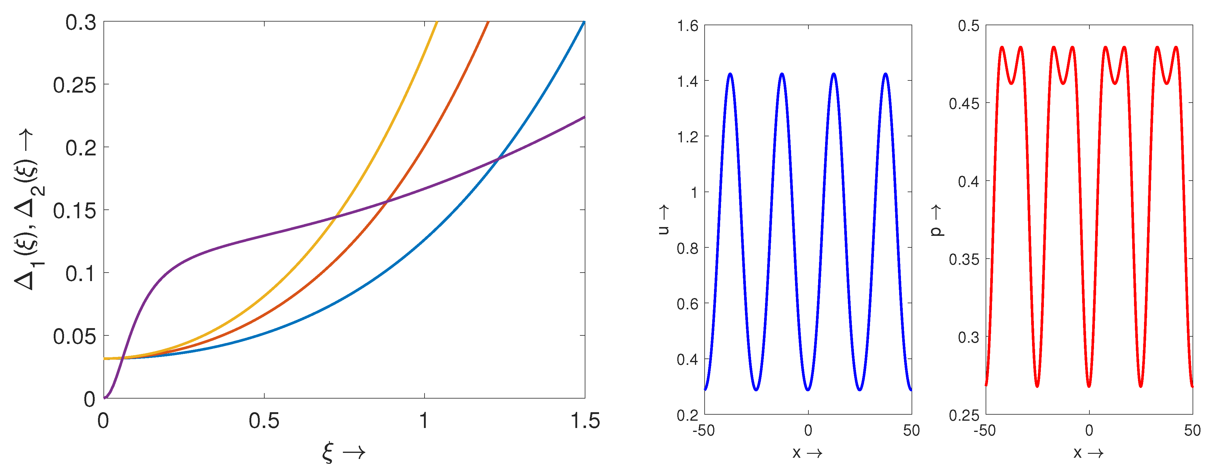
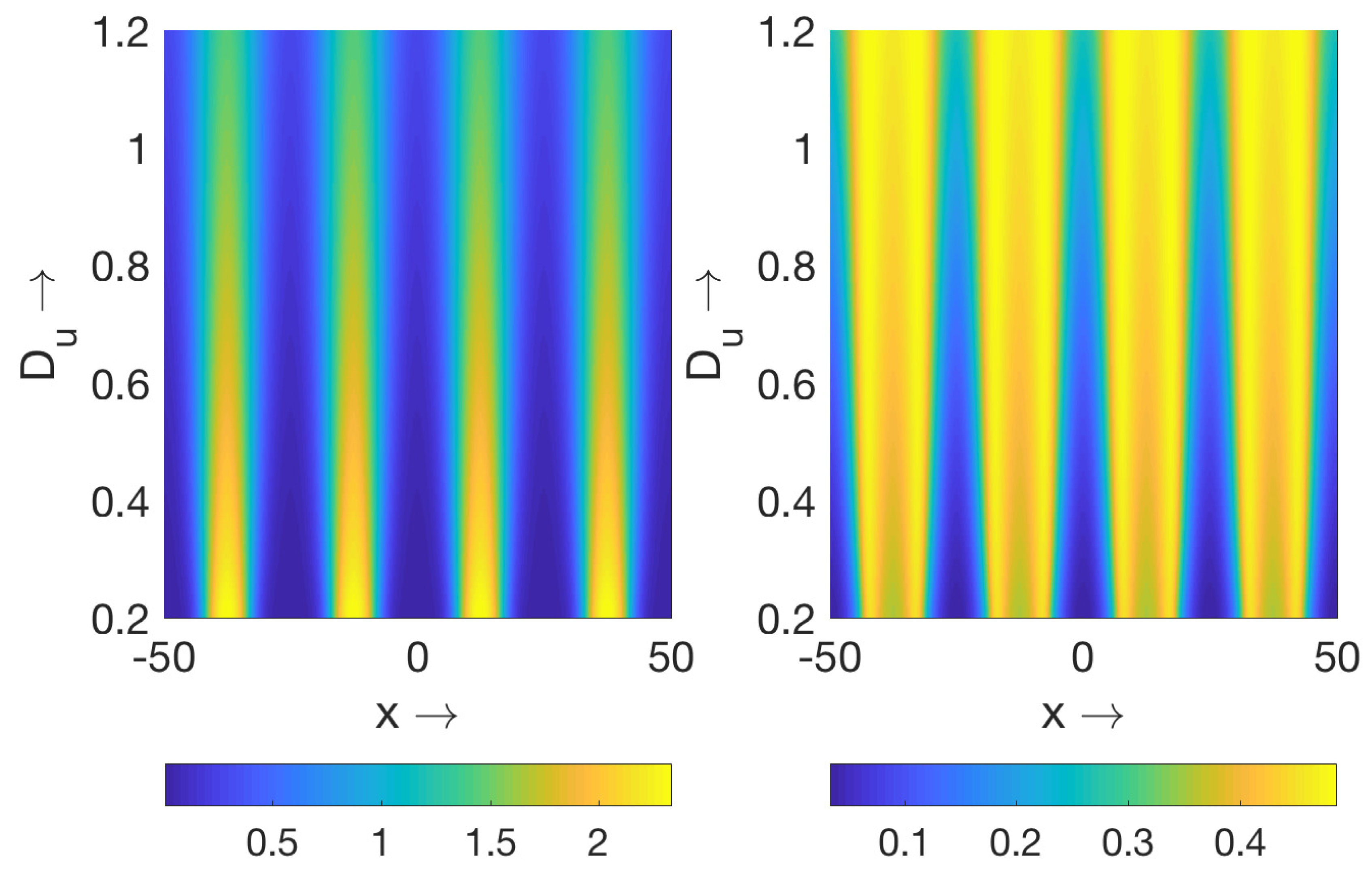
4. Periodic Structures and Pulses for the Wealth-Population System

4.1. Periodic Structures for Nonlocal Consumption

Now we will study the system of two equations
u t = D u 2 u x 2 + f ( u ) p ( 1 k 2 J ( u ) ) k 3 u ,
p t = D p 2 p x 2 + α p ( ψ ( u ) p ) σ 0 p
on the whole real axis, where
f ( u ) = u ( b + u ) 1 + k 1 u , ψ ( u ) = a 2 u u 2 + c 2 2 + σ 1 u α ( 1 + u ) + ψ 0 .
It is similar to system (1) and (2) with the only simplification that the wealth production in Equation (17) is considered to be a linear function of the population density p. This approximation is justified if c 2 is large enough.
The homogeneous-in-space stationary solutions of this system, different from u = 0 , p = 0 can be found from the equations:
f ( u ) ( ψ ( u ) σ 0 / α ) ( 1 k 2 u ) = k 3 u ,
and p = ψ ( u ) σ 0 / α . As before, we assume here that ϕ ( x ) d x = 1 . Equation (19) has a positive solution if k 3 is less than some critical value k 3 * . Denote by u * the maximal solution and assume that it is simple, and set p * = ψ ( u * ) σ 0 / α . We suppose that this solution is stable with respect to the ODE system
d u d t = f ( u ) p ( 1 k 2 u ) k 3 u ,
d p d t = α p ( ψ ( u ) p ) σ 0 p .
Therefore, the eigenvalues of the linearized matrix
A 0 = f ( u * ) p * ( 1 k 2 u * ) k 2 f ( u * ) p * k 3 f ( u * ) ( 1 k 2 u * ) α ψ ( u * ) p * α p *
have negative real parts.
To study the stability of the solution ( u * , p * ) with respect to system (17) and (18), we consider the eigenvalue problem
D u v + f ( u * ) p * ( 1 k 2 u * ) k 3 v k 2 f ( u * ) p * J ( v ) + f ( u * ) ( 1 k 2 u * ) z = λ v ,
D p z + α p * ψ ( u * ) v α p * z = λ z .
The eigenfunction with the components ( v , z ) corresponds to the perturbation of the solution ( u * , p * ) . Here we use that J ( u * ) = u * . Applying the Fourier transform, we obtain the algebraic system of equations
A ( ξ ) v ˜ z ˜ = λ v ˜ z ˜ ,
where tilde denotes the Fourier transform, and
A ( ξ ) = f ( u * ) p * ( 1 k 2 u * ) k 2 f ( u * ) p * ϕ ˜ ( ξ ) k 3 D u ξ 2 f ( u * ) ( 1 k 2 u * ) α ψ ( u * ) p * α p * D v ξ 2 .
Here ϕ ˜ ( ξ ) is the Fourier transform of the kernel ϕ ( x ) of the integral J ( v ) . Let us note that A ( 0 ) = A 0 . Therefore, the eigenvalues of this matrix have negative real parts. We search the values of parameters for which the matrix A ( ξ ) has a positive eigenvalue for some ξ . The critical values of parameters (dispersion relation) is determined by the equality det A ( ξ ) = 0 . Hence, we obtain the following equation:
D u D v ξ 4 T ( A 0 ) ξ 2 + D ( A 0 ) = k 2 f ( u * ) p * ( 1 ϕ ˜ ( ξ ) ) ( α p * + D v ξ 2 ) ,
where T ( A 0 ) = D v a 11 + D u a 22 , a 11 and a 22 are the diagonal elements, and D ( A 0 ) is the determinant of the matrix A 0 . We note that T ( A 0 ) < 0 and D ( A 0 ) > 0 . Therefore, the left-hand side of this equation is positive for all real ξ . Graphical solution of this equation is shown in Figure 5 (left).
The direct analysis of this equation is cumbersome, and we begin with a particular case where ψ ( u * ) = 0 . This condition is satisfied if ψ ( u ) is identically constant. Then the matrix A ( ξ ) has two eigenvalues,
λ 1 ( ξ ) = f ( u * ) f ( u * ) u * p * ( 1 k 2 u * ) k 2 f ( u * ) p * ϕ ˜ ( ξ ) D u ξ 2
and a negative eigenvalue λ 2 ( ξ ) = ( α p * + D v ξ 2 ) . The eigenvalue λ 1 ( ξ ) is similar to the eigenvalue λ ( ξ ) in Section 2.1, and the conditions which determine the equality λ 1 ( ξ ) = 0 are also similar.
Example of numerical simulation of system (17) and (18) is shown in Figure 6. Each horizontal cross section of this figure corresponds to a stationary solution with a given value of D u . The stationary solutions are periodic in space, and the population distribution has a minimum at the maximum of wealth distribution because the function ψ ( u ) decreases for u sufficiently large (Figure 5). It is also interesting to note that decrease of the parameter D u increases the variation of wealth and the total wealth, while the total population decreases. If D p decreases, then both total wealth and total population increase.

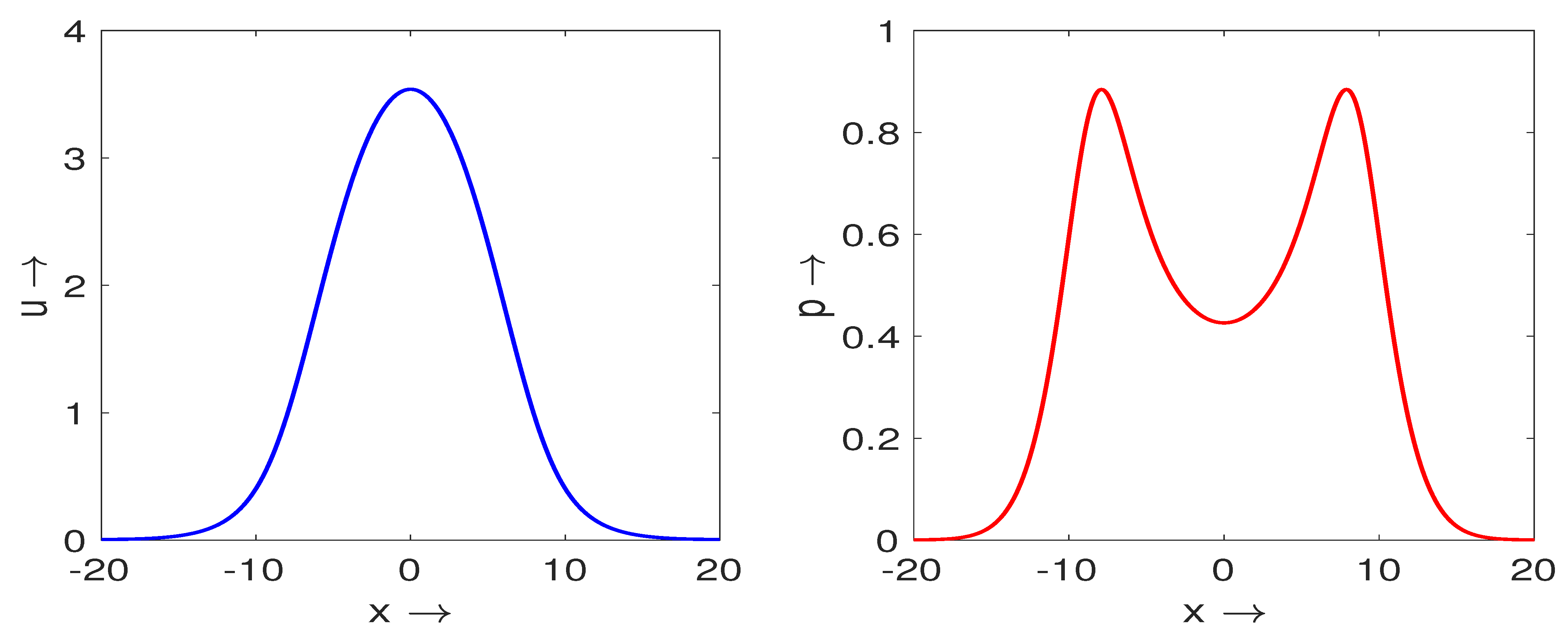
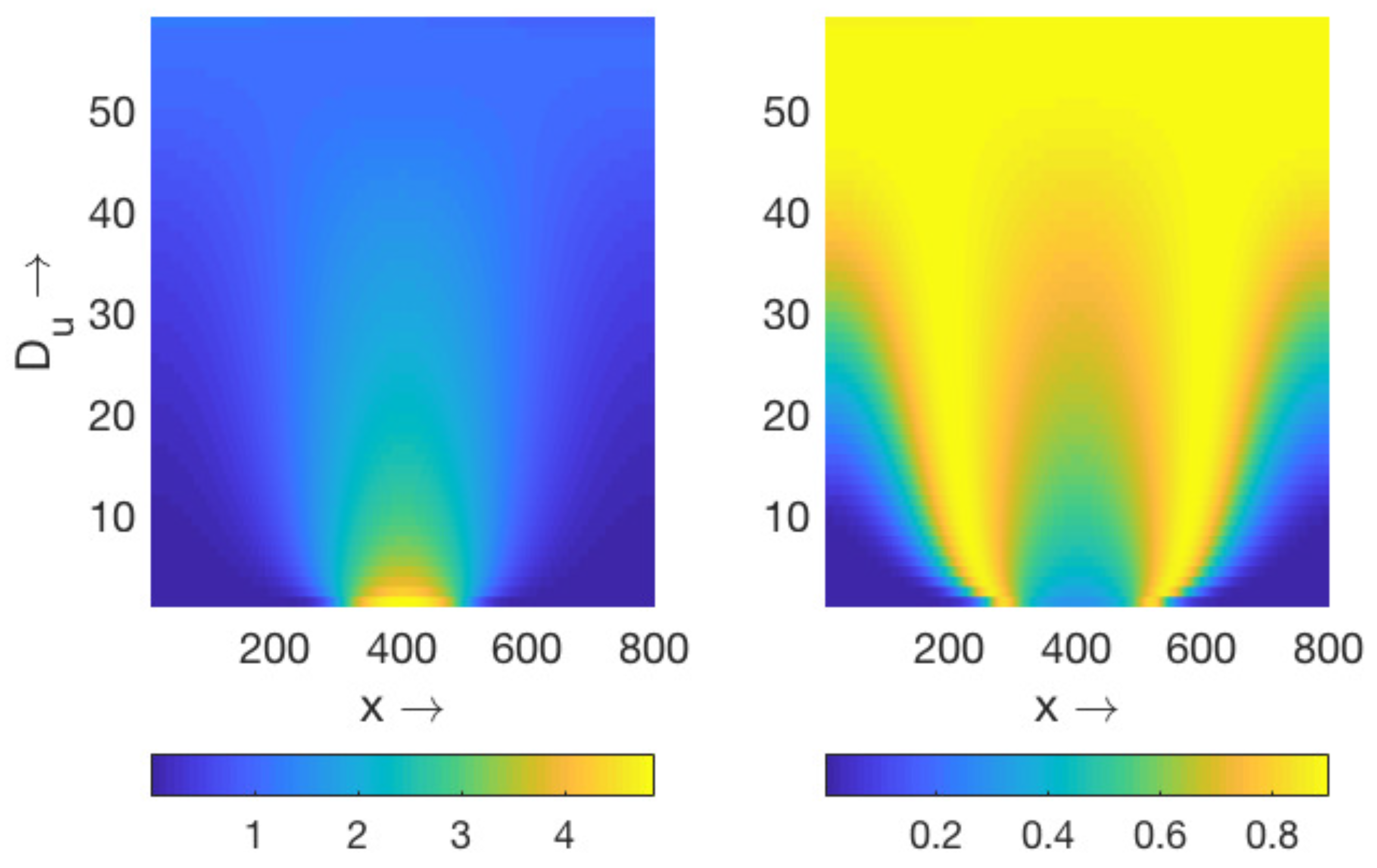
4.2. Pulses for Global Consumption

In this section, we study the case of global consumption for the system of equations
u t = D u 2 u x 2 + f ( u ) p ( 1 k 2 I ( u ) ) k 3 u ,
p t = D p 2 p x 2 + α p ( ψ ( u ) p ) σ 0 p ,
where, as before,
f ( u ) = u ( b + u ) 1 + k 1 u , ψ ( u ) = a 2 u u 2 + c 2 2 + σ 1 u α ( 1 + u ) .
This system is similar to system (17) and (18) where the integral J ( u ) is replaced by I ( u ) . We consider it on a bounded interval 0 < x < L with the Neumann boundary condition. In the stationary case, we have the following boundary value problem:
D u u + f ( u ) p ( 1 k 2 I ( u ) ) k 3 u = 0 ,
D p p + α p ( ψ ( u ) p ) σ 0 p = 0 ,
u ( 0 ) = u ( L ) = 0 , p ( 0 ) = p ( L ) = 0 ,
I ( u ) = 0 L u ( x ) d x (the subscript L in the integral is omitted for brevity). Similar to the nonlocal case considered in the previous section, we consider the maximal positive constant solution ( u * , p * ) and suppose that it is stable with respect to the corresponding ODE system. This solution satisfies the equations
f ( u ) p ( 1 k 2 L u ) k 3 u = 0 , α ( ψ ( u ) p ) σ 0 = 0 ,
where we take into account that I ( u ) = L u .
Linearizing problem (28)–(30) about the solution ( u * , p * ) , we obtain the eigenvalue problem:
D u v + f ( u * ) p * ( 1 k 2 L u * ) v k 3 v k 2 f ( u * ) p * I ( v ) + f ( u * ) ( 1 k 2 L u * ) z = λ v ,
D p z + α p * ψ ( u * ) v α p * z = λ z ,
v ( 0 ) = v ( L ) = 0 , z ( 0 ) = z ( L ) = 0 .
We search a solution of this problem in the form v ( x ) = c 1 cos ( π n x / L ) , z ( x ) = c 2 cos ( π n x / L ) , n = 0 , 1 , 2 , Then we obtain the linear algebraic system of equations:
B c 1 c 2 = λ c 1 c 2 ,
where
B 0 = f ( u * ) p * ( 1 k 2 L u * ) k 3 k 2 L f ( u * ) p * f ( u * ) ( 1 k 2 L u * ) α p * ψ ( u * ) α p * ,
B n = f ( u * ) p * ( 1 k 2 L u * ) k 3 D u ( π n ) 2 / L 2 f ( u * ) ( 1 k 2 L u * ) α p * ψ ( u * ) α p * D p ( π n ) 2 / L 2 ,
n = 1 , 2 , Since ( u * , p * ) is a stable solution of the ODE system, then the eigenvalues of the matrix B 0 have negative real parts. If one of the eigenvalues of the matrix B 1 is positive, then this solution can lose its stability resulting in the bifurcation of a space-dependent solution. Denote the elements of this matrix by b i j , i , j = 1 , 2 . Since b 12 , b 21 > 0 and b 22 < 0 , then det B 1 < 0 if b 11 > 0 . Hence, inequality
f ( u * ) p * ( 1 k 2 L u * ) k 3 D u π 2 / L 2 > 0
provides a sufficient condition for the existence of a positive eigenvalue of the matrix B 1 . This condition is similar to the condition obtained in Section 2.2 for the single equation. It is satisfied for D u sufficiently small or L sufficiently large if
f ( u * ) p * ( 1 k 2 L u * ) k 3 = f ( u * ) f ( u * ) u * p * ( 1 k 2 L u * ) > 0
(see (31)). Condition (35) is not satisfied if the diffusion coefficient D u is sufficiently large. Hence, diffusion stabilizes the constant solution.
If this condition is not satisfied, det B 1 can be still negative. However, if b 11 < 0 and det B 1 > 0 for D u = D p = 0 , then the determinant remains positive in the case of any positive diffusion coefficients. Thus, the origin of the instability is different in comparison with the dissipative (Turing) instability.
Examples
If f ( u ) = u , then condition (36) is not satisfied. If f ( u ) = u 2 , then Equation (31) have a solution for k 3 sufficiently small. In this case, condition (36) is satisfied. An example of wealth and population distributions is shown in Figure 7. Since the function ψ ( u ) decreases for u sufficiently large, then the population distribution has a minimum at the maximum of wealth distribution. Dependence of stationary solutions on the coefficient D u is represented in Figure 8 where each horizontal cross section shows the levels of the corresponding solution. The stationary solution is homogeneous-in-space for large values of D u . Decrease of this parameter leads to the emergence of a non-homogeneous distribution (Figure 7) accompanied by the increase of the total wealth and the decrease of the total population.

5. Discussion and Conclusions

5.1. On the Mechanisms of Pattern Formation

Turing Instability
There are numerous applications where a constant solution is stable as a solution of the corresponding ODE system but it loses its stability with respect to spatial perturbations. The most well-known mechanism of such instability is suggested by A. Turing. It is applicable for reaction–diffusion systems of two or more equations. From the mathematical point of view, this instability can be explained in terms of matrices corresponding to the eigenvalue problem obtained due to linearization about the constant solution. Consider the matrix A ( ξ ) = A 0 D ξ 2 , where the matrix A 0 corresponds to the reaction part of the system, D is the diagonal diffusion matrix with positive diagonal elements, and ξ is the wavenumber of the spatial perturbation. Assuming that all eigenvalues of the matrix A 0 have negative real parts, what can be concluded about the eigenvalues of the matrix A ( ξ ) ? Clearly, if all diagonal elements of the matrix D are equal to each other, then the eigenvalues of the matrix A ( ξ ) have negative real parts for any real ξ . A similar conclusion holds for matrices A 0 with non-negative off-diagonal elements and any diagonal matrix D. However, if off-diagonal elements of the matrix A 0 have variable signs and diagonal elements of the matrix D are different from each other, then the matrix A ( ξ ) can have eigenvalues with positive real parts for some values of ξ . This counterintuitive results is the mathematical basis of the Turing (or dissipative, diffusive) instability. From the physical point of view, this means that diffusion can destabilize a homogeneous-in-space solution, which is stable without diffusion. Turing instability is widely studied in relation to various chemical and biological processes.
Nonlocal Consumption of Resources
Similar mechanisms of pattern formation can manifest themselves for nonlocal reaction–diffusion equations. In this work we consider two of such mechanisms. We will explain them with a model example where the location of the spectrum of the linearized problem is given by the formula
λ ( ξ ) = D ξ 2 + a ϕ ˜ ( ξ ) ,
which represents a simplified version of the spectral curves considered in this work. The first term in the right-hand side of this expression appears in the Fourier transform of the diffusion term, a constant a remains from the reaction term, and ϕ ˜ ( ξ ) is the Fourier transform of the integral kernel ϕ ( x ) . To make the calculations even more explicit, we set ϕ ˜ ( ξ ) = sin ( N ξ ) / ( N ξ ) for the function ϕ 1 ( x ) given by (7). Condition λ ( 0 ) = a 1 < 0 implies the stability of solution without spatial perturbations. Under which conditions λ ( ξ ) can become positive for some real ξ 0 ?
Denote by ξ 0 the point of minimum of the function ϕ ˜ ( ξ ) , ϕ ˜ ( ξ 0 ) < 0 and consider the value λ ( ξ 0 ) = D ξ 0 2 + a ϕ ˜ ( ξ 0 ) . Since a ϕ ˜ ( ξ 0 ) > a 1 , then λ ( ξ 0 ) can be positive even if a 1 < 0 , and the solution becomes unstable with respect to spatial perturbations. Such situation is realized in the case of nonlocal consumption of resources in Section 2.1 and Section 3.1.
The value ξ 0 determines the spatial periodicity of the perturbation. If we consider the problem on a bounded interval, then the real variable ξ takes a discrete set of values ξ k determined by the length of the interval. The frequency ξ k closest to ξ 0 gives the perturbation with the fastest growth.
Global Consumption of Resources
Suppose that
N ξ k = π k , k = 1 , 2 , ,
where N is the same as in the previous paragraph (see also Equation (7)). Then ϕ ( ξ k ) = 0 , λ ( ξ k ) = D ξ k 2 + a , and the maximal eigenvalue λ ( ξ 1 ) = D π 2 + a can be positive if a > 0 and D is sufficiently small. Since ξ k = π k / L to satisfy the boundary conditions, then condition (37) is satisfied for N = L , i.e., in the case of global consumption. In this case, the integral does not change stability without spatial perturbations since λ ( 0 ) = a 1 < 0 but it can change the stability with respect to the spatial perturbations since the integral vanishes on all spatial modes.
There are two differences here in comparison with the previous case: the instability can occur only for a > 0 , and the fastest growing mode corresponds to k = 1 . Therefore, this instability leads to the emergence of pulses contrary to the periodic structures in the nonlocal case.

5.2. Properties of the Nonlocal Economy

The dynamics of human populations are strongly influenced by the wealth distribution through several ways. Increasing wealth can increase the natality, e.g., due to an increase in the household income and hence larger available resources to bring children, but it can also decrease the natality due to a cultural shift; it can decrease the mortality rate provided better health care; and a non-uniform wealth distribution can influence directions and intensity of human migration. Therefore, all these factors should be considered in their interaction. In our previous work, we introduced a novel coupled wealth–population model [23], the properties of its non-spatial counterpart studied in [32] and the emergence of spatial patterns due to the Turing instability analyzed in [24].
In this paper, we further develop wealth–population models by taking into account the dynamic nature of the available resources. Note that by resources we understand not only natural resources such as gas, oil, minerals, etc., but also the production components that results from human activity, e.g., equipment and knowledge. The latter becomes particularly important for modern high-tech products where the intellectual component (software, patents, and so on) can constitute the largest part of the cost of the final product. Moreover, intellectual resources, contrary to natural resources, do not have fixed geographical location. They represent global resources in the sense that the access to them is not spatially dependent, and the cost of their transportation is not a limiting factor for the global economy. Hence, we need to take into account nonlocal effects in the consumption of resources. This is the main objective of this work, and we observe that nonlocal and global economies have quite different properties in comparison with traditional local economies.
An important characteristic of the economy with nonlocal consumption of resources, where the access to resources remains space-dependent but can be sufficiently extended, is the emergence of non-uniform in space wealth distribution. Such structures arise due to the competition for resources if wealth redistribution (diffusion) is sufficiently small. The total wealth in the case of a non-uniform distribution is larger than in the uniform case signifying that nonlocal economy is more efficient than the local one.
In the case of global consumption of resources, where the access to resources is space-independent, a non-uniform distribution can also emerge. Contrary to the previous case, it manifests itself as a single peak in wealth distribution and not as a periodic structure. Hence, global economy can be characterized by a single place of wealth concentration.

5.3. Conclusions and Future Work

Distribution of wealth in space is known to be strongly heterogeneous and this occurs on different spatial scales, ranging from the small scale of separate cities, boroughs, towns and villages to the large scale of states, countries and continents. Although it is not our goal in this paper to provide any quantitative comparison between data and theory, we have been motivated by a few examples where the distribution of wealth across space (e.g., see Figure 1, right) and the distribution of population [24] exhibits features that can be regarded as signs of periodicity. In particular, in North America this suspected periodicity in both wealth and population distribution apparently occurs on the same spatial scale of 1500–2000 km (cf. Figure 1 (right) and Figure 3a in [24]).
In this paper, (see also [24]), we have shown that the emergence of a pattern in the spatial distributions of population and wealth is an inherent property of the corresponding dynamical system. Arguably, this is in a quantitative agreement with some available data (see the previous paragraph). Any quantitative comparison between the theory and the data would require the knowledge of realistic parameter values, which is currently not available; this should become a focus of future research.
We mention here that our model is conceptual and, as such, omits many factors and processes that can, in principle, affect the mechanisms of pattern formation. Transportation costs is one such factor [11]. Another one is the density-dependent diffusion and/or cross-diffusion [23], to allow the population to migrate along the wealth gradient rather than randomly. As the wealth distribution on the small scale is apparently stochastic (cf. Figure 1, left), an inclusion into the model an explicit stochasticity is yet another mathematical challenge. These will become a focus of future research.

Author Contributions

Numerical simulations, M.B.; Model justification, S.V.P.; Model analysis, V.V. All authors have read and agreed to the published version of the manuscript.

Funding

M.B. was supported by SERB grant MTR/2018/000527. V.V. has been supported by the RUDN University Strategic Academic Leadership Program.

Institutional Review Board Statement

Not applicable.

Informed Consent Statement

Not applicable.

Data Availability Statement

Not applicable.

Conflicts of Interest

The authors declare no conflict of interest.

References

  1. Posner, R.A. Equality, Wealth, and Political Stability. J. Law, Econ. Organ. 1997, 13, 344–365. [Google Scholar] [CrossRef]
  2. Von Mises, L. Ideas on Liberty; Foundation for Economic Education: Irvington, NJ, USA, 1955. [Google Scholar]
  3. Okun, A. Equality and Efficiency: The Big Tradeoff; Brookings Institute Press: Washington, DC, USA, 1975. [Google Scholar]
  4. Lansley, S. Inequality and instability: Why more equal societies have more stable economies. Poverty 2012, 142, 10–13. [Google Scholar]
  5. Pareto, V. Cours d’Economie Politique; Librairie Droz: Geneva, Switzerland, 1964. [Google Scholar]
  6. Newman, M.E.J. Power laws, Pareto distributions and Zipf’s law. Contemp. Phys. 2005, 46, 323–351. [Google Scholar] [CrossRef] [Green Version]
  7. Quadrini, V.; Rios-Rull, J.-V. Understanding the U.S. Distribution of Wealth. Fed. Reserve Bank Minneap. Q. Rev. 1997, 21, 22–36. [Google Scholar]
  8. Davies, J.B.; Shorrocks, A.F. The distribution of wealth. In Handbook of Income Distribution; Elsevier: Amsterdam, the Netherlands, 2000; Volume 1, pp. 605–675. [Google Scholar]
  9. Epstein, J.M. Nonlinear Dynamics, Mathematical Biology, and Social Science; Addison-Wesley: Reading, MA, USA, 1997. [Google Scholar]
  10. Turchin, P. Historical Dynamics: Why States Rise and Fall; Princeton University Press: Princeton, NJ, USA, 2003. [Google Scholar]
  11. Krugman, P. Confronting the mistery of urban hierarchy. J. Japan. Intern. Econ. 1996, 10, 399–418. [Google Scholar] [CrossRef] [Green Version]
  12. Fujita, M.; Krugman, P.R.; Venables, A. The Spatial Economy: Cities, Regions, and International Trade; MIT Press: Cambridge, MA, USA, 1999. [Google Scholar]
  13. Bouchaud, J.-P.; Mézard, M. Wealth condensation in a simple model of economy. Physica 2000, 282, 536–545. [Google Scholar] [CrossRef] [Green Version]
  14. Wang, N. An equilibrium model of wealth distribution. J. Monet. Econ. 2007, 54, 1882–1904. [Google Scholar] [CrossRef] [Green Version]
  15. Ikeda, K.; Murota, K. Bifurcation Theory for Hexagonal Agglomeration in Economic Geography; Springer: Tokyo, Japan, 2014. [Google Scholar]
  16. Torregrossa, M.; Toscani, G. On a Fokker-Planck equation for wealth distribution. Kinet. Relat. Model. 2018, 11, 337–355. [Google Scholar] [CrossRef] [Green Version]
  17. Chenevert, R.; Gottschalck, A.; Klee, M.; Zhang, X. Where the Wealth Is: The Geographic Distribution of Wealth in the United States. US Census Bureau, 2017. Available online: https://www.census.gov/content/dam/Census/newsroom/press-kits/2017/assa-geographic-distr-wealth.pdf (accessed on 10 October 2020).
  18. Rammelt, C.F.; van Schie, M.; Tegabu, F.N.; Leung, M. Vaguely Right or Exactly Wrong: Measuring the (Spatial) Distribution of Land Resources, Income and Wealth in Rural Ethiopia. Sustainability 2017, 9, 962. [Google Scholar] [CrossRef] [Green Version]
  19. Murray, J.D. Mathematical Biology; Springer: Berlin/Heidelberg, Germany, 1989. [Google Scholar]
  20. Cantrell, R.S.; Cosner, C. Spatial Ecology via Reaction-Diffusion Equations; John Wiley & Son: London, UK, 1989. [Google Scholar]
  21. Malchow, H.; Petrovskii, S.V.; Venturino, E. Spatiotemporal Patterns in Ecology and Epidemiology: Theory, Models, and Simulation; CRC Press: Boca Raton, FL, USA, 2008. [Google Scholar]
  22. Meron, E. Nonlinear Physics of Ecosystems; CRC Press: Boca Raton, FL, USA, 2015. [Google Scholar]
  23. Volpert, V.; Petrovskii, S.; Zincenko, A. Interaction of human migration and wealth distribution. Nonlinear Anal. 2017, 159, 408–423. [Google Scholar] [CrossRef] [Green Version]
  24. Zincenko, A.; Petrovskii, S.; Volpert, V. Turing Instability in an Economic-Demographic Dynamical System Can Lead to Pattern Formation on Geographical Scale. arXiv 2020, arXiv:2006.01664v1. [Google Scholar]
  25. Deaton, A. The Great Escape—Health, Wealth, and the Origins of Inequality; Princeton Univ Press: Princeton, NJ, USA, 2013. [Google Scholar]
  26. Rees, W.E. Ecological footprints and appropriated carrying capacity: What urban economics leaves out. Environ. Urban. 1992, 4, 121–130. [Google Scholar] [CrossRef]
  27. Small, M.L.; Harding, D.J.; Lamont, M. Reconsidering culture and poverty. Ann. Am. Acad. Political Soc. Sci. 2010, 629, 6–27. [Google Scholar] [CrossRef]
  28. Groth, C. Lecture Notes in Macroeconomics; Mimeo: New York, NY, USA, 2015. [Google Scholar]
  29. The Digital Economist. Available online: http://www.digitaleconomist.org/dmacro.html (accessed on 10 October 2020).
  30. Volpert, V. Elliptic partial differential equations. In Reaction-Diffusion Equations; Birkhäuser: Basel, Switzerland, 2014; Volume 2. [Google Scholar]
  31. Genieys, S.; Volpert, V.; Auger, P. Pattern and waves for a model in population dynamics with nonlocal consumption of resources. Math. Model. Nat. Phenom. 2006, 1, 63–80. [Google Scholar] [CrossRef] [Green Version]
  32. Zincenko, A.; Petrovskii, S.; Volpert, V. An economic-demographic dynamical system. Math. Model. Nat. Phenom. 2018, 13, 27. [Google Scholar] [CrossRef]
Figure 1. Wealth distribution in the USA quantified by different measures and at different spatial scale: median household income on the county scale (by the courtesy of STATS America, left) and the Gini coefficient on the state scale (adapted from [17], right). Please note that the map shown in the right figure exhibits signs of periodicity in a longitudinal direction, e.g., along the black curve.
Mathematics 09 00351 g001
Figure 2. (Left): eigenvalues λ ( ξ ) for f ( u ) = u 2 , k 2 = 1 , k 3 = 1 / 8 , u * = 0.854 , D = 0.2 , μ = 1 (lower curve), μ = 0.17 (middle curve), μ = 0.1 (upper curve). (Right): numerical simulations of Equation (5) with the periodic boundary conditions and the exponential function ϕ 2 ( x ) for the same values of parameters as in the linear stability analysis. The figure shows the converges of solution with the initial condition localized at the center of the interval to a stationary periodic-in-space solution. Different colors show the level lines of solution on the ( x , t ) -plane.
Mathematics 09 00351 g002
Figure 3. (Left): example of a pulse solution obtained by numerical simulations of Equation (9) with the periodic boundary conditions for the values of parameters: b = k 1 = 0 , k 2 = 0.02 , k 3 = 0.125 and D = 2.5 (red), D = 2 (green), D = 1.5 (magenta), D = 1 (black), D = 0.5 (blue). (Right): periodic-in-space stationary solutions for different values of the diffusion coefficient for the values of parameters b = k 1 = 0 , k 2 = 1 , k 3 = 0.125 .
Mathematics 09 00351 g003
Figure 4. The function W ( D ) (left) and multiple stationary solutions (right) for the values of parameters: b = k 1 = 0 , k 2 = 1 , k 3 = 0.125 , D = 0.5 (for the right figure).
Mathematics 09 00351 g004
Figure 5. Graphical solution of the dispersion relation (24) (left) with its left-hand side Δ 1 ( ξ ) for three different values of D u : 0.1 (blue), 0.2 (red), 0.3 (yellow) and the right-hand side Δ 2 ( ξ ) (violet) which is independent of D u . The values of other parameters are as follows: k 2 = 1 , k 3 = 0.125 , μ = 0.1 , α = 1 , a 2 = 1 , c 2 = 1 , σ 0 = 0.01 , σ 1 = 0.0 , D p = 0.2 , ψ 0 = 0.1 . Wealth (middle) and population (right) distributions in the case of nonlocal consumption obtained by numerical simulations of system (17) and (18) for the same values of parameters as for Figure 6 and D u = 0.8 and other values of parameters: b = 0 , k 1 = 0 , k 2 = 1 , k 3 = 0.125 , σ 0 = 0.01 , σ 1 = 0 , ψ 0 = 0 , α = 1 , a 2 = 1 , c 2 = 1 , D p = 0.2 , and μ = 0.1 (exponential kernel).
Mathematics 09 00351 g005
Figure 6. Wealth (left) and population (right) distributions in the case of nonlocal consumption obtained by numerical simulations of system (17) and (18) with the periodic boundary conditions for different values of D u and other values of parameters: b = 0 , k 1 = 0 , k 2 = 1 , k 3 = 0.125 , σ 1 = 0.01 , α = 1 , a 2 = 1 , c 2 = 1 , D p = 0.2 , and μ = 0.1 (exponential kernel). For each value of D u , the horizontal cross section of the figure indicates the color scale of the corresponding stationary solution.
Mathematics 09 00351 g006
Figure 7. Example of wealth (left) and population (right) distributions in the case of global consumption obtained by numerical simulations of system (26) and (27) for the values of parameters: D u = D p = 0.2 , b = k 1 = 0 , k 2 = 0.02 , k 3 = 0.125 , α = 1 , σ 0 = 0.1 , a 2 = 2 , c 2 = 1 .
Mathematics 09 00351 g007
Figure 8. Wealth (left) and population (right) distributions in the case of global consumption obtained by numerical simulations of system (26) and (27) with the periodic boundary conditions for different values of D u and other values of parameters: D p = 0.2 , b = k 1 = 0 , k 2 = 0.02 , k 3 = 0.125 , α = 1 , σ 0 = 0.1 , a 2 = 2 , c 2 = 1 , ψ 0 = 0 . For each value of D u , the horizontal cross section of the figure indicates the color scale of the corresponding stationary solution.
Mathematics 09 00351 g008
Publisher’s Note: MDPI stays neutral with regard to jurisdictional claims in published maps and institutional affiliations.

