A Neural Network-Based Approach for Approximating Arbitrary Roots of Polynomials ^†

Abstract

Finding arbitrary roots of polynomials is a fundamental problem in various areas of science and engineering. A myriad of methods was suggested to address this problem, such as the sequential Newton’s method and the Durand–Kerner (D–K) simultaneous iterative method. The sequential iterative methods, on the one hand, need to use a deflation procedure in order to compute approximations to all the roots of a given polynomial, which can produce inaccurate results due to the accumulation of rounding errors. On the other hand, the simultaneous iterative methods require good initial guesses to converge. However, Artificial Neural Networks (ANNs) are widely known by their capacity to find complex mappings between the dependent and independent variables. In view of this, this paper aims to determine, based on comparative results, whether ANNs can be used to compute approximations to the real and complex roots of a given polynomial, as an alternative to simultaneous iterative algorithms like the D–K method. Although the results are very encouraging and demonstrate the viability and potentiality of the suggested approach, the ANNs were not able to surpass the accuracy of the D–K method. The results indicated, however, that the use of the approximations computed by the ANNs as the initial guesses for the D–K method can be beneficial to the accuracy of this method.

1. Introduction

Finding arbitrary (real or complex) roots of a given polynomial is a fundamental problem in different areas of science and engineering. Applications of root-finding emerge from, e.g., control and communication systems, filter design, signal and image processing, and codification and decodification of information.

Although many iterative methods for finding all the roots of a given polynomial already exist, e.g., the Newton’s method and the Durand–Kerner (D–K) method [1,2], they usually require: (a) repeated deflations, which may cause very inaccurate results because of the accumulation of floating point rounding errors, (b) good initial approximations to the roots for the algorithm converge, or (c) the computation of first or second order derivatives, which, besides being computationally intensive, it is not always possible.

Due to those drawbacks, and since traditional Artificial Neural Networks (ANNs) are generally known for their capability to discover complex nonlinear input–output mappings, and consequently find good approximations for complex problems, this paper suggests and tests a neural network-based approach for finding real and complex roots of polynomials, aiming to assess its potential and limitations regarding efficiency and accuracy. (It is important to note that this approach uses inductive inference in order to find the roots of a given polynomial simultaneously.) The ANN-based approach is then compared with the D–K method, one of the most traditional simultaneous iterative methods for finding all the roots of a given polynomial. Finally, the approximations computed by the ANNs are used as an initialization scheme for the D–K method.

The first works about finding the roots of a given polynomial with ANN-based approaches started in 1995, when Hormis and colleagues [3] presented the $\sum -\prod$ ANN with the objective of separating a two-dimensional polynomial into two one-dimensional polynomials (with the same degree). In 2001, Huang and Chi [4,5] used that ANN architecture and added a priori knowledge about the relationships between the roots and coefficients in the training algorithm aiming to find the real and complex roots of a given polynomial. (This is considered by the authors to be the first work that addressed the root-finding problem using ANNs directly.)

In 2003, a dilatation method for finding close arbitrary roots of polynomials was suggested [6] and had the objective of magnifying the distance between close roots, allowing them to be found more easily by ANNs. On the other hand, Huang et al. [7,8] integrated the root moment method and the Newton identities into the ANN training algorithm.

Mourrain and colleagues [9] then investigated the determination of the number of real roots of polynomials using a Feedforward Artificial Neural Network (FNN) and concluded that the ANNs were capable of performing such task with high accuracy. Zhang et al. [10] suggested using a discrimination system in order to compute the number of distinct real or complex roots or, in other words, the roots’ multiplicities. They used the ANN structure proposed by Huang and Chi [4,5].

Das and Seal [11] proposed a completely different approach using a set of divisors of the polynomial coefficients, denoted here as D. In this view, if r is a divisor of D and a divisor of the coefficient of the lowest degree term, then r is a potential root of the specific polynomial. The coefficients of the considered polynomial are fed into an ANN by the input neurons, and then the first hidden neuron in the first hidden layer separates the coefficients list into two other lists. Each list serves as input for the two hidden neurons in the second hidden layer. These two nodes compute the divisor of its coefficients in parallel, and those that are also divisors of the coefficient of the highest degree term are passed to the next two hidden neurons of the next hidden layer, who are responsible for improving the candidate roots using a learning algorithm.

Nevertheless, the approaches mentioned above do not make use of the inductive inference capacity of ANNs to compute an approximation for each root of a given polynomial. This is the focus of this study. This paper is organized as follows: after the introduction, Section 2 describes the methodology followed to find the approximations for arbitrary roots of a polynomial using ANNs and the D–K method. Section 3, in turn, presents the comparative results between the ANN-based approach trained with two optimization algorithms and the D–K method. In addition, in the same section, the ANN-based approach is tested as an initialization scheme for the D–K method. This paper ends with a section dedicated to conclusions.

The work presented in this paper is an extended version of the work by the authors presented at the International Conference on Mathematical Applications [12], in which the study was focused on the use of ANNs for finding the real roots of a given polynomial. Here, however, the main aim is to find both real and complex polynomial roots.

2. Materials and Methods

The generation of the training and test data sets is described in this section, together with the way ANNs were trained in order to compute approximations to arbitrary (real or complex) roots of polynomials. The main focus of this study is to compute approximations of the roots ${\alpha }_i(i=1,\dots ,n)$ of an n-th degree real univariate polynomial $P\left(x\right)=a_n{x}^n+a_{n-1}{x}^{n-1}+\dots +a_{1}x+a_0$ with real and complex roots, given its real coefficients. In this study, only the values $5,10,15,20$ and 25 for n were considered.

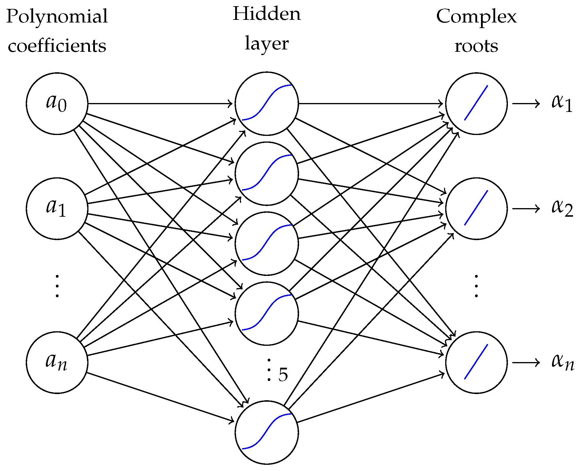
The block diagram of this approach is presented in Figure 1, and it shows that the coefficients of a given polynomial are used as the inputs for the ANNs that are then processed by the network and used to output an approximation for each root. It is important to note that, according to the Fundamental Theorem of Algebra [13], an n-th degree polynomial has n real or complex roots. Thus, a priori, the number of output nodes is known.

The results were then compared in terms of accuracy and in terms of execution time with the D–K method described below.

2.1. Durand–Kerner Algorithm

The D–K method [1,2], also known in the literature as Weierstrass’ or Weierstrass–Dochev’s method [14], is a traditional iterative method for computing approximations to all real or complex roots of a polynomial simultaneously. Although the application of this method does not involve the calculation of derivatives, it requires a good initial approximation to each of the roots (which must be generated using another iterative method) for the convergence of the algorithm.

Let $P\left(x\right)=a_n{x}^n+a_{n-1}{x}^{n-1}+\cdots +a_{1}x+a_0$$(a_n\ne 0)$ be a real polynomial of degree n. The D–K method for this generic polynomial is given by [15]:

$${\displaystyle x_i^{(k+1)}=x_i^{\left(k\right)}-\frac{P\left(x_i^{\left(k\right)}\right)}{{\displaystyle a_n\prod _{\begin{array}{c}j=1\\ j\ne i\end{array}}^n(x_i^{\left(k\right)}-x_j^{\left(k\right)})}},}$$

(1)

where $i=1,\dots ,n$ is the root index and k is the current iteration number.

The convergence order of the D–K method in the general case is known to be quadratic for simple roots, but is only linear for multiple roots [16].

It is also important to note that the formulation of the D–K iterative process allows the method to compute both the real and complex roots of a given polynomial. Therefore, if the imaginary part of a root is lower than a predefined threshold, then the root is considered a real root.

For computing the initial approximations for the D–K method, the simple and well-known Cauchy’s bound [17] was used, since it provides an upper bound ($ub$) for the modulus of the polynomial roots, which, in the case of a real polynomial $P\left(x\right)$, is given by:

$$ub=1+max\left\{\left|{\displaystyle \frac{a_0}{a_n}}\right|,\cdots ,\left|{\displaystyle \frac{a_{n-2}}{a_n}}\right|,\left|{\displaystyle \frac{a_{n-1}}{a_n}}\right|\right\}.$$

(2)

In other words, the Cauchy’s upper bound defines a disk of radius $ub$ centred at the origin of the complex plane that includes all real and complex roots of the polynomial. In this view, the initial root values for an n-th degree real univariate polynomial, here denoted by ${\alpha }_i^{\left(0\right)}(i=1,\dots ,n)$, will be set randomly inside a circle with radius equal to $ub$, i.e.:

$${\alpha }_i^{\left(0\right)}=cos\left(\theta \right)\times ub+sin\left(\theta \right)j\times ub,$$

(3)

where $j=\sqrt{-1}$ and $\theta$ given by:

$$\theta =r\times \pi \times 2,$$

(4)

with r being a random number between 0 and 1.

Later in this paper, the approximations computed by the ANNs were also used as an initialization scheme for the D–K method.

2.2. Artificial Neural Networks

In this study, five neural networks (one for each polynomial degree chosen) composed by three layers (input, hidden, and output layer) were trained employing the well-known Levenberg–Marquardt Algorithm (LMA) and Particle Swarm Optimization (PSO). The inputs for the networks were the real coefficients of a set of polynomials of degrees 5, 10, 15, 20, and 25, and the outputs were the polynomial roots, as can be seen in Figure 1. In this figure, ANN n denotes the neural network that can output approximations to the roots of a real n-th degree polynomial.

2.2.1. Data Sets

Table A1. Head of the input data set for training the ANN 5 for computing both real and complex roots.

${\mathit{a}}_{\mathbf{0}}$	${\mathit{a}}_{\mathbf{1}}$	${\mathit{a}}_{\mathbf{2}}$	${\mathit{a}}_{\mathbf{3}}$	${\mathit{a}}_{\mathbf{4}}$	${\mathit{a}}_{\mathbf{5}}$
0.6489	0.5608	0.0764	0.9170	0.6737	0.0856
0.1398	0.8675	0.6737	0.7915	0.6805	0.3244
0.8254	0.8206	0.5198	0.7785	0.8128	0.0229
0.1884	0.4211	0.5824	0.0200	0.9023	0.7577
0.4004	0.5791	0.8399	0.8190	0.9042	0.2391
︙	︙	︙	︙	︙	︙

and

Table A2. Head of the output data set for training the ANN 5 for computing both real and complex roots.

Re(α1)	Im(α1)	Re(α2)	Im(α2)	Re(α3)	Im(α3)	Re(α4)	Im(α4)	Re(α5)	Im(α5)
−6.1207	0.0000	−1.8031	0.0000	−0.8277	0.0000	0.4406	−0.7973	0.4406	0.7973
−1.1952	−0.8191	−1.1952	0.8191	0.1822	0.0000	0.2375	−1.0345	0.2375	1.0345
−34.5703	0.0000	−0.8836	−0.4828	−0.8836	0.4828	0.4004	−0.9324	0.4004	0.9324
−1.4203	0.0000	−0.3379	−0.3584	−0.3379	0.3584	0.4527	−0.7189	0.4527	0.7189
−2.9534	0.0000	−0.6260	0.5992	−0.6260	0.5992	0.2114	−0.8430	0.2114	0.8430
︙	︙	︙	︙	︙	︙	︙	︙	︙	︙

in Appendix A show the head of the data sets (with 100,000 records) that were used with ANN 5 to compute approximations for the real and complex roots. In the second data set, corresponding to the roots, the odd and even columns represent respectively the real and the complex parts of the root values, i.e.:

$${\alpha }_i=\left\{\mathrm{Re}\left({\alpha }_i\right),\mathrm{Im}\left({\alpha }_i\right)\right\},i=1,\dots ,n.$$

(5)

To generate the data sets, the coefficients of the polynomials were first generated randomly in the interval $[0,1]$, and from these the exact (real or complex) roots were calculated using a symbolic computation package. Thus, the ANN does not know a priori which roots are real or complex. It is important to note here that double-precision values were used to generate these data sets although coefficients and roots are shown with only four decimal places.

From these data sets, $70\%$ of the samples were used to train the ANNs. The remaining $30\%$ was used to test the generalization capabilities of the ANNs by computing a performance measure on samples that were not used to train the ANNs.

2.2.2. Architecture

For this study, shallow FNNs were used and, after several tests performed according to some “rule of thumb” methods available in the literature for obtaining the optimal number of hidden neurons and hidden layers [18,19,20], it was found that the resulting network architectures did not vary significantly in terms of accuracy. Taking this into account, in this experimental study, the hidden layer was always composed by ten neurons for all the final tests.

Besides that, the hyperbolic tangent sigmoid (tansig) activation function [21] was applied only in the hidden layer, and it was chosen to guarantee that values remain within a relatively small range (in this case $[-1,1]$) and, through the application of an anti-symmetric sigmoid (S-shaped) transfer function, to allow the network to learn nonlinear relationships between coefficients and roots. In the output layer, no activation function was embedded, since the final rescaled output is still a linear function of the original data, allowing the ANNs to output values that are not circumscribed to the range of values of the activation function.

It is important to note that a min-max normalization method [22] was used to rescale data to the range $[-1,1]$ in order to improve the convergence properties of the training algorithm [23].

The architecture of the ANN is represented in Figure 2. However, it is important to emphasize that two output units were used for each root: one for the real part and the other for the imaginary part. In other words, ANN 5 has ten outputs—five for the real part and five for the imaginary part—ANN 10 has 20 outputs, and so on.

2.2.3. Training Algorithms

The well-known LMA [24,25] was used for the ANNs training. The LMA is known due to its efficacy and convergence speed, being therefore one of the fastest methods for training FNNs, particularly medium-sized ones. A more detailed description on the use of LMA for training ANNs is presented, e.g., in [26,27], since its details go beyond the scope of this work.

Moreover, LMA is a hybrid algorithm that combines two optimization algorithms, which are the Gauss–Newton method (because of its efficacy) and the gradient descent method (due to its robustness). At each minimization step, the Levenberg–Marquardt algorithm makes one of these methods more or less dominant by means of a non-negative algorithmic parameter ($\lambda$) that is adjusted at each iteration [28].

The weights of the synaptic connections are then updated according to the difference between the predicted and the observed value, backpropagating that error according to:

$$w^{(k+1)}=w^{\left(k\right)}-{\left({\left(J^{\left(k\right)}\right)}^T·J^{\left(k\right)}+{\lambda }^{\left(k\right)}I\right)}^{-1}·\left({\left(J^{\left(k\right)}\right)}^T·e^{\left(k\right)}\right),$$

(6)

where I is the identity matrix and e is the squared error vector between the target values and the estimated values. Finally, J is a Jacobian matrix given by $J_{i,j}={\displaystyle \frac{\partial e_i}{\partial w_{j·}}}$.

The LMA was used following a batch learning strategy, meaning that the network’s weights and biases are updated after all the samples in the training set are presented to the network.

This training algorithm is known for being a successful algorithm even if it starts in a zone far from the optimal one. However, the calculation of the Jacobian matrix may cause some performance issues in the algorithm, especially in deep ANNs, ANNs with many hidden neuron units, or big data sets [29].

The PSO algorithm [30,31] was also used as a training algorithm, since it has a good ability to explore the search space. In addition, the calculations needed for the algorithm’s execution are far more simple and expected to be less computationally demanding when compared to the LMA.

The LMA is considered an exact method since it uses the derivative information to optimize the weights of the ANN in order to minimize the error between the exact target values and the estimated target values. The PSO algorithm, on the other hand, uses particles that explore stochastically the search space with $(10+32n)$ dimensions, each one corresponding to each synaptic connection between the neuron units in an ANN with one hidden layer. For example, for the ANN 25, 260 weights are needed to connect the input layer to the hidden layer—26 coefficient neurons × 10 hidden neurons. On the other hand, 550 synaptic connections are required in order to connect the hidden neurons and one bias neuron to the nodes in the output layer, i.e., $(10+1)$ hidden neurons with bias × 25 × 2 neurons for the real and imaginary parts of a complex root. This defines a search space with 810 dimensions to optimize using PSO.

In order to explore the search space, PSO uses particles, which correspond to candidate solutions. Each particle has a velocity and a position, and is able to exchange information about the best positions found (according to a cost function) during the search process with all particles in the swarm (which is known as a gbest model), or with a set of neighboring particles (a model that is known as lbest). In this optimization technique, each particle has a memory mechanism that enables it to store two types of information: the best position found by the other particles (social information), and also the best position found by the particle itself (cognitive information). In this way, a usual strategy for defining the equations of motion of each particle i in the swarm at every iteration k is given by [32,33]:

$$\left\{\begin{array}{c}{\overrightarrow{V}}_i^{(k+1)}=K\left[{\overrightarrow{V}}_i^{\left(k\right)}+{\phi }_1{R_1}_i^{\left(k\right)}\left({\overrightarrow{p}}_i^{\left(k\right)}-{\overrightarrow{x}}_i^{\left(k\right)}\right)+{\phi }_2{R_2}_i^{\left(k\right)}\left({\overrightarrow{g}}^{\left(k\right)}-{\overrightarrow{x}}_i^{\left(k\right)}\right)\right],\hfill \\ {\overrightarrow{x}}_i^{(k+1)}={\overrightarrow{x}}_i^{\left(k\right)}+{\overrightarrow{V}}_i^{(k+1)},\hfill \end{array}\right.$$

(7)

where ${\phi }_1$ and ${\phi }_2$ are respectively the cognitive and the social weights, controlling how much the particle’s own experience and the swarm’s experience should influence the particle’s movement, whereas $R_1$ and $R_2$ are uniformly distributed random vectors between the search space boundaries, being responsible for adding diversity to the swarm and thus they try to lessen the premature converge of the algorithm to a local optimum point.

Lastly, ${\overrightarrow{p}}_i^{\left(k\right)}$ and ${\overrightarrow{g}}^{\left(k\right)}$ denote the personal best position of the particle i and the current global best position of the swarm at iteration k, respectively. Finally, K is a constriction term [32,33], given by:

$$K={\displaystyle \frac{2}{|2-\phi -\sqrt{{\phi }^2-4\phi }|}},$$

(8)

where $\phi ={\phi }_1+{\phi }_2$ and $\phi >4$. Typically, $\phi =4.1$, and thus $K\approx 0.7298$.

For optimizing the ANN’s weights, and thus minimizing the cost function defined for both training algorithms as being the Mean Squared Error (MSE), each particle corresponds to an ANN with a configuration of weights different from the configuration of each of the other particles in the swarm. The PSO then proceeds normally until a stopping criterion is met. In this case, the algorithm stops when it reaches the maximum number of iterations (5000 iterations) or when the MSE derived from the training data set is lower than a predefined $ϵ$ (in this case, $ϵ={10}^{-12}$).

3. Results and Discussion

In this section, the results obtained with the adopted approach are presented, along with comparisons with the numerical approximations provided by the D–K method, in terms of accuracy and execution time, when the polynomials have real and complex roots.

As a measure of accuracy, the authors opted to use the MSE. The MSE is computed as follows:

$$\mathrm{MSE}=\frac{1}{n}\sum _{i=1}^n{(D_i-N_i)}^2,$$

(9)

where $D_i$ denotes the actual i-th root value ($i=1,\dots ,n$) in the test data set, and $N_i$ is the corresponding approximation obtained with the D–K method or the proposed ANN approach.

Since the proposed approach computes the real and the imaginary parts separately, the results produced by the D–K method were also split into its real and imaginary parts, in order to allow for comparing the results obtained in both ways.

It is important to note that the D–K method and the ANNs training used the same stopping criteria, i.e., a maximum number of iterations equal to 5000 and $ϵ={10}^{-12}$ (which means that the value of the polynomial, when evaluated on the position of the root found, is less than or equal to ${10}^{-12}$).

As already mentioned, in order to compute the MSE, $30\%$ of the original data set entries were reserved, and the new data set thus produced contains entries randomly chosen that were not employed to train the networks. It should be also pointed out that all the ANNs were trained 20 times and, based on the lowest MSE on the test data set, only one was chosen to be compared to the numerical approximations produced by the D–K method.

The results on the execution time for both methods were obtained using a personal computer equipped with a 7th generation Intel Core i7 processor and 16 GB of RAM.

3.1. Levenberg–Marquardt Algorithm

Table 1. Comparison between the ANN approach and the D–K method in terms of MSE for polynomials with real and complex roots.

Degree	ANN MSE	D–K MSE
5	36.5387	$4.9290\times {10}^{-09}$
10	386.7120	$3.4800\times {10}^{-09}$
15	2.7157	$2.6766\times {10}^{-09}$
20	146.2455	$1.8608\times {10}^{-09}$
25	4.6057	$9.7454\times {10}^{-10}$

shows the MSE for each of the five polynomial degrees, and these error values indicate that the ANN approach does not yet surpass the accuracy of the D–K method that always finds the roots with an accuracy greater than $1\times {10}^{-8}$. It is also possible to depict that, when the ANNs are trained with the LMA, the method failed to converge, in all the trials, to reasonably accurate results. In addition, the MSE is not related to the degree of the polynomial, since polynomials of degree 10 had a worse MSE when compared to the results for polynomials of the 15th degree.

Table 2. Comparison between the ANN approach and the D–K method in terms of the average execution time (in seconds) for polynomials with real and complex roots.

Degree	ANN	D–K
5	0.018	0.0842
10	0.015	0.4098
15	0.027	1.2728
20	0.025	3.0516
25	0.028	5.4552

, on the other hand, shows that the execution time with ANN remains almost constant when the degree of the polynomial increases. The opposite happens with the D–K method, with which an increase in the degree of the polynomial implies an increase in the execution time. This result was already expected because computing polynomial roots using the D–K method, unlike ANN, is a pure iterative procedure.

Considering that accurate results were not achieved when using the ANN-based approach for computing the real and complex polynomial roots using the real and imaginary parts of the roots in the test data sets, the roots were transformed into polar coordinates, in order to assess its impact on the accuracy of the approach, i.e.:

$${\alpha }_i^{\prime }=\left\{\sqrt{x^2+y^2},{tan}^{-1}\left({\displaystyle \frac{y}{x}}\right)\right\},$$

(10)

where x and y correspond to the real and imaginary parts of ${\alpha }_i$, respectively.

However, and as can be seen in

Table 3. MSE for the ANN-based approach for polynomials with real and complex roots in polar coordinates.

Degree	MSE
5	678.9594
10	249.7066
15	210.9323
20	146.6783
25	114.6380

, the MSE obtained is even higher for most of the polynomials’ degrees when compared to the previous approach.

Interestingly, in this approach, polynomials with a higher degree had a lower MSE. Nevertheless, for all the polynomial degrees, the LMA was not successful in updating the ANNs’ weights in order to reduce the MSE.

In conclusion, the ANNs trained with the LMA showed to have limitations in terms of accuracy when compared to the D–K method. However, this approach surpassed the efficiency of the D–K method, since the ANN-based approach required a lower execution time in all the tests carried out when compared with the D–K method.

3.2. Particle Swarm Optimization

In this section, the results of the ANN approach trained with the PSO algorithm are presented.

The structure, i.e., the number of neuron units in the hidden layer and the activation functions of the ANN, as well as the data sets, were kept the same as in the previous sections in order to enable a fair comparison between the two approaches: ANN trained with the LMA and ANN trained with the PSO algorithm. Although it has not been investigated in this work, it is important to note that the PSO algorithm could also be used to obtain the optimal ANN architecture that best minimizes the difference between the observed and the expected values.

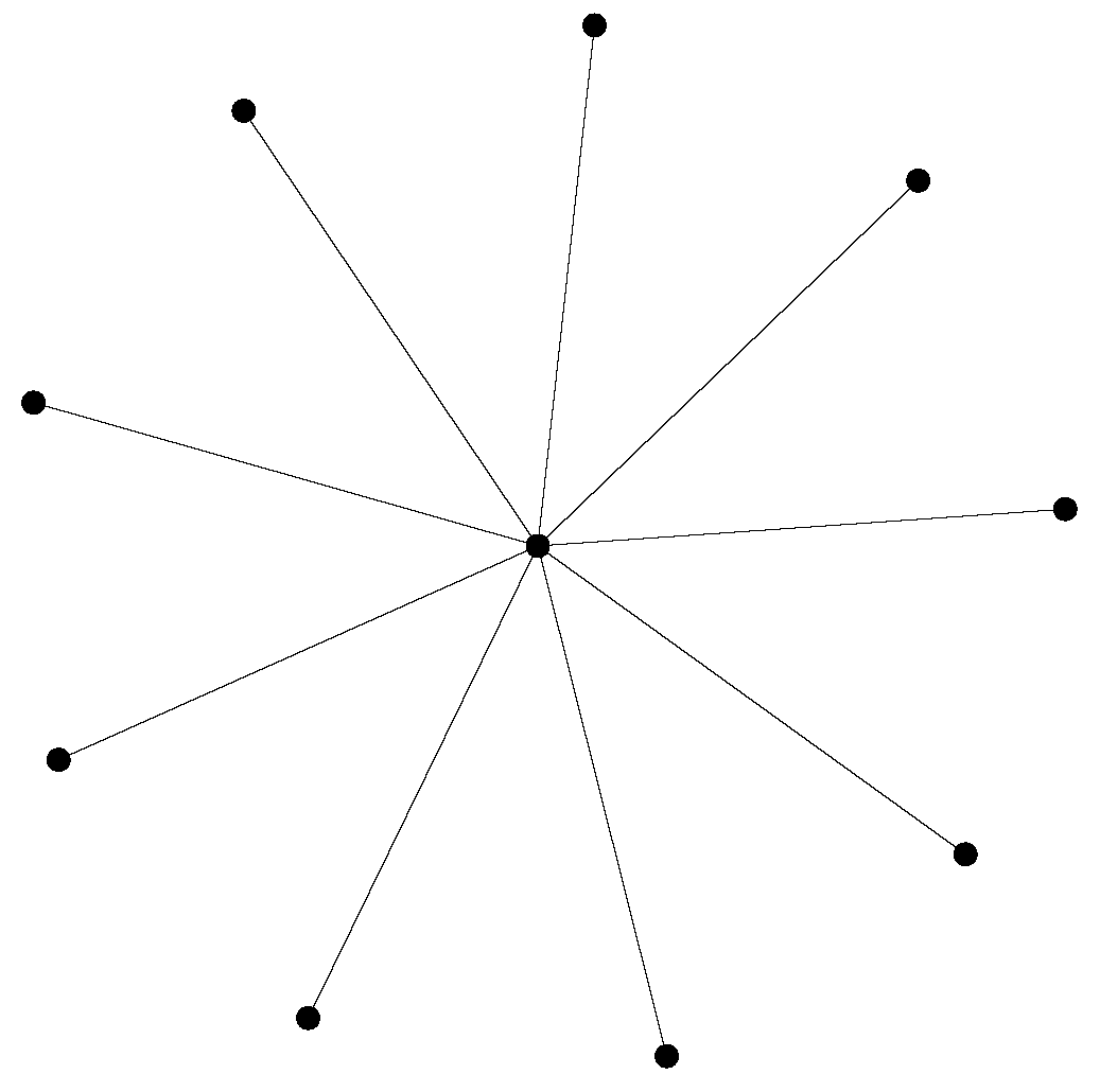
The PSO algorithm was initialized with a swarm of 24 particles, organized in a star topology, with the motion equation given by Equation (7) (with ${\phi }_1={\phi }_2=2.05$). In a swarm with a star communication structure, particles are independent (i.e., isolated from each other), except for a central particle (known in the literature as the focal point) that intermediates the communication between the particles.

As illustrated in Figure 3, the central particle knows the performance of every particle in the swarm and changes its position according to the best particle’s position. If its new position is better than the previous best global position, then the central particle is responsible for spreading this discovery [34,35].

Thus, the star communication structure is centralized, since the central particle is influenced and is the only particle that influences the remaining particles. This structure was chosen because it has a lower converge speed when compared to other neighborhood topologies (e.g., mesh, toroid, and ring), and consequently a higher probability of achieving good results, since the algorithm will explore the search space better, and thus escape from local minima.

For each ANN, 20 tests were executed and, for each experiment, the MSE was computed as Equation (9). Nevertheless, only the ANN with the lowest MSE was kept for comparison. The MSE results are presented in

Table 4. MSE comparison for the D–K method and the ANN-based approach trained with LMA and PSO for polynomials with real and complex roots.

Degree	D–K MSE	LMA MSE	PSO MSE
5	$4.9290\times {10}^{-09}$	36.5387	0.0036
10	$3.4800\times {10}^{-09}$	386.7120	0.0069
15	$2.6766\times {10}^{-09}$	2.7157	0.0083
20	$1.8608\times {10}^{-09}$	146.2455	0.0121
25	$9.7454\times {10}^{-10}$	4.6057	0.0111

.

When compared with the ANNs trained with the LMA, training the ANNs using PSO represents a significant improvement in terms of accuracy, as can be depicted in Table 4. Besides that, it is possible to observe that, as the degree of the polynomial increase, the accuracy of the ANN trained using PSO is little affected, except for the case of polynomials of degree 20 and 25. Nevertheless, polynomials of degree 20 and 25 showed a similar MSE value.

Similarly, the accuracy of the results obtained with the ANN-based approach for computing both real and complex roots in polar coordinates was also improved by training the ANN with the PSO algorithm when compared to the LMA. The results of this approach, presented in

Table 5. MSE comparison for the ANN-based approach trained with LMA and PSO for polynomials with real and complex roots in polar coordinates.

Degree	LMA MSE	PSO MSE
5	678.9594	0.0159
10	249.7066	0.0253
15	210.9323	0.0343
20	146.6783	0.0344
25	114.6380	0.0397

, show that the use of the PSO algorithm produced a stable MSE, especially for higher degree polynomials.

It is noteworthy that converting the complex roots to polar coordinates resulted, for all the polynomial degrees considered, in a loss of generalization capabilities. Thus, the real and imaginary parts should be used, along with the ANN trained using the PSO algorithm, in order to compute both real and complex roots of a given polynomial.

This comparison allowed for concluding that the ANN trained with the PSO algorithm seems to be a more effective alternative when compared to the training using the LMA, since it was able to provide a better generalization (and, consequently, to produce lower MSEs). As noted by Mendes et al. [36], one possible justification for the fact of the PSO has surpassed the LMA generalization capabilities may be related to the number of local minima present in the search space, since the PSO algorithm revealed to be the best training algorithm when a high number of local minima exist.

Besides that, even for higher degree polynomials, the ANN trained with the PSO algorithm revealed a modest MSE. It is worth mentioning that, since all the MSE values presented in Table 1 are significantly less than one, it can be inferred that the networks have a good capacity to generalize the space of results. Thus, with some confidence, it is possible to conclude that the networks are able to solve any real univariate polynomial (at least of the degrees considered) with real and complex roots.

However, these results are again limited, especially when compared to that obtained with the D–K method. With this in mind, the next section suggests making use of the ANN-based approach trained with the PSO algorithm as an initialization scheme for the D–K method.

3.3. Initialization Scheme for the Durand–Kerner Method

This section is intended to focus on the use of the ANN-based approach, trained with the PSO algorithm, for computing the initial guesses for the roots to be used with the D–K method. This section appears due to the fact that the results obtained from the ANN-based approach were not superior to the ones computed by the D–K method. Taking this into consideration, instead of competing, the ANN-based approach can help to leverage the effectiveness and efficiency of the D–K method.

As already mentioned, the D–K method requires good initial approximations for all roots in order to converge. Thus, the objective of this section is to compare the use of the D–K method when it is initialized using the Cauchy’s upper bound or by using the ANNs introduced in the previous section.

Results will be compared in terms of the MSE, execution time, number of iterations, and effectiveness. In its turn, the effectiveness is computed by dividing the number of times that the D–K method found the roots of a given polynomial by the total number of tests. It is also important to note that all the presented results correspond to the average of the different tests that were run.

Like in the previous sections, and, for the sake of comparison, only the test data set containing the coefficients and polynomial roots will be used.

Table 6. Comparison between the Cauchy’s bound and the ANN-based approach in providing initial approximations to the D–K method.

	Degree	MSE	Exec. Time	No. Iterations	Effectiveness
Cauchy’s upper bound	5	$4.9290\times {10}^{-09}$	0.0842	67.5155	$99.82\%$
	10	$3.4800\times {10}^{-09}$	0.4098	83.1480	$99.77\%$
	15	$2.6766\times {10}^{-09}$	1.2728	103.4006	$99.72\%$
	20	$1.8608\times {10}^{-09}$	3.0516	127.3676	$99.68\%$
	25	$9.7454\times {10}^{-10}$	5.4552	143.9964	$99.58\%$
ANN	5	$4.5822\times {10}^{-09}$	0.1008	77.7170	$99.84\%$
	10	$2.7444\times {10}^{-09}$	0.6589	105.5521	$99.67\%$
	15	$1.4705\times {10}^{-09}$	2.3469	151.4759	$99.43\%$
	20	$9.2850\times {10}^{-10}$	4.3203	184.3320	$99.33\%$
	25	$4.8588\times {10}^{-10}$	8.6969	226.1478	$99.01\%$

presents a comparison between the Cauchy’s upper bound and the ANN-based approach for the case when the polynomials have real and complex roots.

The comparison between the Cauchy’s upper bound and ANN-based approach leads to the conclusion that the ANN-based approach can be used only to improve the accuracy of the D–K method, surpassing the Cauchy’s upper bound in all tests. However, if one is interested in enhancing the performance of the algorithm, then the use of the D–K method with the initialization scheme based on the Cauchy’s upper bound should not be discarded, taking into account that, for all polynomial degrees, this strategy required a shorter execution time and a smaller number of iterations.

Moreover, in terms of effectiveness, the Cauchy’s upper bound strategy was superior to the ANN-based approach, especially for higher degree polynomials. Thus, it can be concluded that the ANN-based approach can be used only to improve the accuracy of the D–K method.

Finally, this section shows that the ANN-based approach trained with PSO can be used as an initialization scheme for the D–K method, since it found, on average, more accurate roots when compared to the initialization scheme based on the Cauchy’s bound. However, one should choose the Cauchy’s upper bound if the aim is to improve efficiency of the D–K method.

4. Conclusions

This paper introduces an approach for computing approximations for the real and complex roots of a given polynomial, based on the inductive inference capabilities of the ANNs. Results were then compared in terms of effectiveness and efficacy to the D–K method.

The authors started by training the ANNs using the LMA algorithm and as input the coefficients of the polynomials considered. The weights of each ANN were then updated based on the error between the true root values and the values produced by the ANN, i.e., the approximations to the roots of the polynomials. Although the LMA was unable to converge to an acceptable solution, the results were significantly improved to an acceptable accuracy by using PSO as a training algorithm. Results, however, still showed that ANNs were not able to surpass the accuracy of the D–K method. Nevertheless, the ANN approach presented advantages in terms of performance.

As an example of the use of this approach, the authors tested the applicability of the ANNs as an initialization scheme for the D–K method, and reached the conclusion that the ANN-based approach is a viable alternative when compared to the initialization scheme based on the Cauchy’s upper bound, especially in terms of accuracy.

Finally, it will be important that future research compare the proposed approach with other simultaneous iterative methods for polynomial root-finding, such as the accelerated D–K method [37,38], the well-known Ehrlich–Aberth method [39,40], the accelerated Ehrlich method [37], or even more recent methods for the simultaneous determination of polynomial roots. Besides that, it is also important to compare other approaches for computing the initial approximations for the roots of a given polynomial based on its coefficients [39,41,42,43], as well as considering some special classes of polynomials in addition to randomly generated polynomials.