A Clustering Perspective of the Collatz Conjecture

Abstract

This manuscript focuses on one of the most famous open problems in mathematics, namely the Collatz conjecture. The first part of the paper is devoted to describe the problem, providing a historical introduction to it, as well as giving some intuitive arguments of why is it hard from the mathematical point of view. The second part is dedicated to the visualization of behaviors of the Collatz iteration function and the analysis of the results.

1. Introduction

The Collatz problem is one of the most famous unsolved issues in mathematics. Possibly, this interest is related to the fact that the question is very easy to state, but very hard to solve. In fact, it is even complicated to give partial answers. The problem addresses the following situation.

Consider an iterative method over the set of positive integers $\mathbb{N}$ defined in the following way. If $n\in \mathbb{N}$ is even, then we consider the positive integer $\frac{1}{2}n$ for the next step. On the other hand, if $n\in \mathbb{N}$ is odd, then we consider the positive integer $3n+1$ for the next step. The Collatz conjecture states that, independently of the chosen initial value for $n\in \mathbb{N}$, the number 1 is reached eventually.

Remark 1.

Observe that, in the case that Collatz conjecture does not hold, there is a positive integer $a\in \mathbb{N}$ such that:

• The orbit of a is unbounded, i.e., ${\lim }_{n\to \infty }{C}^n\left(a\right)=\infty$.
• The orbit of a is periodic and non-trivial, i.e., there is $N\in \mathbb{N}$ such that $C^N\left(a\right)=a$, for $a\ne 1,2,4$.

Remark 2.

Indeed, it is possible to study and provide representations of the second possibility in Remark 1. Observe that, essentially, this second possibility deals with the existence of a positive integer solution to certain linear equations modulo $2^N$. This idea is developed in Section 2, and it is used to describe some interesting relations and graphical representations.

In [1], we can find a discussion concerning the origin of the problem. During the 1930s, Lothar Collatz took an interest in the iterations of some number-theoretic functions. Indeed, it is possible to find a similar problem to the Collatz conjecture in his notebook in 1932. It is also known, and it has been confirmed by many other mathematicians, that Collatz discussed several problems of this kind in the International Congress of Mathematicians in 1950 (Cambridge, MA, USA). Nevertheless, it is not clear whether the $3n+1$ problem was mentioned in these discussions or not. In any case, what is clear is that the problem spread rapidly during that decade. According to Richard Guy and Shizuo Kakutani, the problem was studied in Cambridge and Yale for some time between the lately 1950s and the early 1960s, but with no remarkable results. In the last 50 years, the mathematical community has tried different approaches to the Collatz conjecture, but none of them is believed to provide a definitive path that would allow to solve the problem. Possibly, it should be adequate to highlight contributions in two directions:

• On the one hand, there are theoretical arguments that allow proving statements which are similar to the conjecture, but a bit weaker. In this sense, we can find the contributions in [2,3].
• On the other hand, there are numerical experiments that show that the conjecture holds for numbers which are smaller than a certain threshold $N\in \mathbb{N}$, or that the Collatz functions does not have non-trivial cycles with length less or equal to $m\in \mathbb{N}$. The values of m and N have been continuously improved, and, nowadays, we can ensure that the conjecture holds for $N<5.78\times {10}^{18}$ (see [1]) or that the length of a non-trivial cycle is, at least, $1.7\times {10}^7$ (see [4]). These computational arguments have been feeding continuously the opinion that the Collatz conjecture is true, and that there is no non-trivial cycle.

Besides, some authors have devoted efforts to rewrite the conjecture in other terms (see, e.g., [5] for an approach in terms of algebraic and boolean fractals). Furthermore, some work has been developed concerning the representation and study of the Collatz conjecture in terms of graphs [6,7,8,9,10,11,12].

The visualization of the Hailstone sequences is often performed by means of directed graphs. However, while these representations produce simple to read plots, the question arises on how the ‘rules’ adopted for the graphical representation put some additional conditions on the final plot. Having this idea in mind, we propose the adoption of two clustering computational techniques, namely the hierarchical clustering (HC) and multidimensional scaling (MDS) methods, for computational clustering and visualization [13,14,15,16,17,18,19,20,21]. The first produces graphical portraits of data known as dendrograms and trees in a two-dimensional space, while the second consists of point loci. In practical terms, the MDS set of points are plotted in either two- or three-dimensional charts. These computational schemes have been adopted successfully in a number of scientific areas and allow unveiling patterns embedded in the dataset [22,23,24,25,26]. For the case of MDS, the possibility of having three dimensions allows an additional degree of freedom that is of utmost importance when handling complex phenomena.

This paper is organized as follows. Section 2 discusses the Collatz conjecture and the difficulties posed by this apparently simple problem. Section 3 introduces the MDS technique and analyzes the results for the Hailstone sequences. Finally, Section 4 summarizes the main conclusions.

2. Why Is Collatz Problem Difficult?

There are several reasons that could be considered enough to claim that the Collatz conjecture is a really difficult mathematical problem. Probably, one of the most important ones is that it has been a popular problem for at least fifty years and it has not been solved yet. Nevertheless, there are heuristic arguments that can give a hint on why it is complicated to provide an answer, or why the most reasonable paths for facing the problem end up in nothing.

Observe that, due to Remark 1, to prove the Collatz conjecture, it would be enough to ensure that there are neither unbounded orbits nor non-trivial cycles for the Collatz iteration map.

2.1. Number Theory Arguments

We give a hint on why would it be very hard to prove the Collatz conjecture with standard number theory arguments. If we imagine that the Collatz problem would admit non-trivial periodic orbits, then we would be able to find $a\in \mathbb{N}$ and $N\in \mathbb{N}$ such that $C^N\left(a\right)=a$. First, we show how these equations look for small values of $N\in \mathbb{N}$.

The equation $C\left(n\right)=n$ reads

$$\begin{array}{c}\hfill \frac{n}{2}=n, \mathrm{if} n\equiv 0\left(\mathrm{mod}2\right),\\ \hfill 3·n+1=n, \mathrm{if} n\equiv 1\left(\mathrm{mod}2\right).\end{array}$$

(1)

The equation $C^2\left(n\right)=n$ reads

$$\begin{array}{c}\hfill \frac{n}{4}=n, \mathrm{if} n\equiv 0\left(\mathrm{mod}4\right),\\ \hfill 3·\frac{n}{2}+1=n, \mathrm{if} n\equiv 2\left(\mathrm{mod}4\right),\\ \hfill \frac{3·n+1}{2}=n, \mathrm{if} n\equiv 1,3\left(\mathrm{mod}4\right).\end{array}$$

(2)

The equation $C^3\left(n\right)=n$ reads

$$\begin{array}{c}\hfill \frac{n}{8}=n, \mathrm{if} n\equiv 0\left(\mathrm{mod}8\right),\\ \hfill 3·\frac{n}{4}+1=n, \mathrm{if} n\equiv 4\left(\mathrm{mod}8\right),\\ \hfill \frac{3·\frac{n}{2}+1}{2}=n, \mathrm{if} n\equiv 2,6\left(\mathrm{mod}8\right),\\ \hfill \frac{3·n+1}{4}=n, \mathrm{if} n\equiv 1,5\left(\mathrm{mod}8\right),\\ \hfill 3·\frac{3·n+1}{2}+1=n, \mathrm{if} n\equiv 3,7\left(\mathrm{mod}8\right).\end{array}$$

(3)

We observe that, for small values of $m\in \mathbb{N}$, the study of the equation $C^m\left(n\right)=n$ can be divided into the study of $F_{m+1}$ linear equations with constraints modulo $2^m$, where $F_k$ is the kth Fibonacci number. This can be generalized for arbitrarily large values of m, as follows.

First, observe that any linear equation would be

$${\displaystyle {◯}_{j=1}^m{f}_{k_j}\left(n\right)=n,}$$

(4)

where $n\in \mathbb{N}$, $k_j\in \{0,1\}$, $f_0\left(n\right)=n/2$, $f_1\left(n\right)=3n+1$ and ◯ denotes the composition operator. Thus, in principle, we would have as many expressions for $C^m\left(n\right)$ as different choices for $\overrightarrow{k}:=(k_1,\dots ,k_m)\in {\{0,1\}}^m$, but we recall that not all choices for $\overrightarrow{k}$ are possible. Indeed, it is not possible to apply $f_1$ two times in a row without any $f_0$ between them, since, given any odd number n, the resulting number $f_1\left(n\right)=3·n+1$ will always be even. Hence, in general, the number of equations $C^m\left(n\right)=n$ will be strictly fewer than the obvious estimate $2^m$.

Why is $F_{m+1}$ the number of possible linear equations for $C^m\left(n\right)=n$? As mentioned above, for small values of m, we have already checked this property. To provide a rigorous proof for larger values of m, we only need to use mathematical induction. Suppose that we know that for $C^{m-2}\left(n\right)=n$ we have $F_{m-1}$ equations. It is always possible to apply $f_0$ to each of the $F_{m-1}$ left-hand sides, getting $F_{m-1}$ new equations for $C^{m-1}\left(n\right)=n$. Besides, we get some additional equations by applying $f_1$ to some of the left-hand sides (not all of them). Due to the induction hypotheses, this $f_1$ can be applied to $F_m-F_{m-1}$ left-hand sides. Hence, for $F_{m-1}$ equations that appear in $C^{m-1}\left(n\right)=n$, we can apply either $f_0$ or $f_1$, and, for $F_m-F_{m-1}$ equations, we can only apply $f_0$. In conclusion, we have $F_{m+1}=2·F_{m-1}+F_m-F_{m-1}$ equations for $C^m\left(n\right)=n$.

Why does each equation appearing in $C^m\left(n\right)=n$ have some constraint modulo $2^m$? Again, we can use a mathematical inductive argument in order to clarify this point. If we assume that all equations appearing in $C^{m-1}\left(n\right)=n$ have certain constraints modulo $2^{m-1}$, and since we can determine $C\left(n\right)$ modulo $2^{m-1}$, provided we know n modulo $2^m$, then it is clear that all equations in $C^m\left(n\right)=C^{m-1}\left(C\left(n\right)\right)=n$ have some constraints modulo $2^m$.

According to the two previous paragraphs, seeking non-trivial cycles is equivalent to looking for non-trivial solutions to one of these $F_{m+1}$ linear equations with constraints modulo $2^m$. If we forget about the modular condition, each of these equations has a unique solution. Besides, it would be possible to compute these solutions inductively, after developing a recurrence that computes the new solutions in terms of the previous ones. After doing this, the idea would be to use some argument involving integer arithmetic (congruences, p-adic valuations, etc.) in order to show that the equation does not admit solutions apart from 1, 2 and 4. This attempt would fail, since the Collatz iteration map is known to have more cycles than $(4,2,1)$ when defined on integer numbers, allowing negative values. Thus, there is no clear obstruction in terms of elementary number theory for having solutions to $C^m\left(n\right)=n$ different from $n\in \{1,2,4\}$.

2.2. Probabilistic Arguments

Other possible way to face the problem would be the following one. Suppose that we are given a number in the Collatz sequence that has been obtained after applying the map $f_1$: What is the expected contraction factor of such a number until we apply $f_1$ again? Observe that, in the case that such a factor would be smaller than $\frac{1}{3}$, one could try to develop probabilistic arguments ensuring that any number eventually shrinks in size and arrives to the trivial cycle. In the case that such a factor would be larger than $\frac{1}{3}$, one could try to develop probabilistic arguments showing that unbounded sequences do exist.

After applying $f_1$, we have a number n which is known to be even. Thus, at least we will apply $f_0\left(n\right)=n/2$ one time. Indeed, the number n will be even, but not a multiple of 4, with probability $1/2$. Analogously, it will be a multiple of 4, but not a multiple of 8, with probability $1/4$, etc. Observe that, if n is a multiple of $2^s$, but not $2^{s+1}$, then we will apply $f_0$ exactly s times. Thus, the expected value of the iteration of n which is previous to the step of applying $f_1$ is:

$$\sum _{j=1}^{\infty }\frac{1}{2^j}·\frac{n}{2^j}=n·\sum _{j=1}^{\infty }\frac{1}{4^j}=\frac{n}{3}.$$

Hence, in probabilistic terms, the Collatz iteration map is expected to neither shrink nor expand a number in the long-term.

3. Clustering Analysis and Visualization

3.1. Hierarchical Clustering

The HC is a computational technique that assesses a group of N objects in a n-dim space $\mathcal{A}$ and portrays them in a graphical representation highlighting their main similarities under the light of some metric [16,27].

The method starts by gathering the dataset $\mathcal{A}$ that characterizes the phenomenon in some sense. Usually, we obtain a number N of objects having a high dimensional nature which makes its analysis difficult. The next step is to define some metric for comparison of all objects between themselves. It is possible to adopt measures of similarity or, alternatively, of ‘distance’. We adopt distances d that obey the axioms of: (i) identity of indiscernibles $d\left(x,y\right)=0\iff x=y$; (ii) symmetry and sub-additivity $d\left(x,y\right)=d\left(y,x\right)$; and (iii) triangle inequality $d\left(x,y\right)\le d\left(x,z\right)+d\left(z,y\right)$, where $x,y,z\in \mathcal{A}$. Based on this metric, an $N\times N$ matrix $D=\left[d_{ij}\right]$, $i,j=1,\dots ,N$, of object-to-object distances is constructed. The matrix D is symmetric and has main diagonal with zeros when adopting distances. The HC uses the input information in matrix D and produces a graphical representation consisting in a dendrogram or a hierarchical tree.

The HC requires using either the agglomerative or divisive clustering iterative computational scheme. In the first, each object starts in its own cluster and the algorithm merges the most similar items until having just one cluster. In the second, all objects start in a common cluster and the algorithm separates them until each has its own cluster. In both schemes, a linkage criterion, based on the distances between pairs, is required for calculating the dissimilarity between clusters. The maximum, minimum and average linkages are possible criteria [28]. The clustering quality can be assessed by means of the cophenetic correlation [29]. When the cophenetic correlation is close to 1 (to 0), we have a good (weak) cluster representation of the original data. In Matlab, the cophenetic correlation is computed by means of the command cophenet. Nonetheless, we adopt the agglomerative clustering and the average-linkage [30,31], with the program Phylip http://evolution.genetics.washington.edu/phylip.html, for processing the matrix of distances D.

3.2. Multidimensional Scaling

The MDS is a computational technique that tries to reproduce and visualize in a space of dimension n objects described in a space of dimensional $m>n$, where the objects are represented by points.

The MDS algorithm tries to reproduce the original distances by calculating a $N\times N$ matrix $\tilde{\Delta }=\left[{\tilde{d}}_{ij}\right]$ so that the replicated distances $\tilde{d}$ minimize some quadratic index, called stress S. Consequently, the problem is converted to a numerical optimization of some index such as $S={\left[{\sum }_{i,j=1,\dots ,N}{\left(d_{ij}-{\tilde{d}}_{ij}\right)}^2\right]}^{1/2}$ and we obtain a set of N objects in a space of dimension n that approximate the original ones. Usually, users adopt $n=2$ or $n=3$ since they allow a direct visualization. We adopt $n=3$ because the plots allow better approximations than the simper case of $n=2$, but this requires some rotation, shift and amplification for obtaining the best perspective of the visualization.

The obtained loci of objects is called a ‘map’ and the quality can be assessed by means of the so-called Sheppard and stress plots. The first one draws the original versus the replicated distances. A low/high scatter means a good/poor match between the distances. Moreover, a collection of points near a 45 degree straight (curved) line means a linear (non-linear) relationship. Nonetheless, in both cases, the key point is to have a low scatter. The second tool for assessing the MDS quality consists of the plot of S versus n. Usually, we obtain a monotonic decreasing curve with a significant reduction of S after the initial values. The final step of the process requires the user to analyze the MDS map since the axes have no physical meaning and there is no a priori assignment of some good/bad or high/low interpretation to the coordinate values of the points.

The interpretation of the map must have in mind the clusters that may emerge and the patterns formed by the points. This interpretation is not based on an ascetic perspective, but rather in the sense that they reflect some relationship embedded in the original dataset. The user can test several distances because each one may have its owns merits and drawbacks in capturing the characteristics of the phenomena under study. In other words, these loci are usually different since each one follows a distinct metric. Consequently, we can have more than one distance producing a ‘good’ MDS map. On one hand, this means that we may have to test a number of distances to obtain an eclectic overview, while, on the other hand, we may use more than one map to visualize and interpret the results.

We calculate the MDS technique using the Matlab classical multidimensional scaling command cmdscale.

3.3. The Adopted Computational Algorithm

Hereafter, we apply the HC and MDS techniques to unravel the evolution of the Hailstone sequences. For capturing the dynamics of the Hailstone sequences, we record the successive numbers until reaching the final value of 1. To have vectors of identical length all remaining values are considered 0. Finally, the vectors are ordered in the inverse sequence. This means that, for example, number 6 is represented as the vector $x=(1,2,4,8,16,5,10,3,6,0,\dots ,0)$. We consider a test-bed of six distances, namely the ArcCosine, Manhattan, Euclidean, Canberra, Clark and Lorentzian, given by [32,33]:

$$\begin{array}{ll}{d}_{AC}& =\arccos \frac{{\displaystyle \sum _{k=1}^m{x}_i\left(k\right)x_j\left(k\right)}}{\sqrt{{\sum }_{k=1}^m{x}_i{\left(k\right)}^2{\sum }_{k=1}^m{x}_j{\left(k\right)}^2}},\end{array}$$

(5a)

$$\begin{array}{ll}{d}_{Ma}& ={\displaystyle \sum _{k=1}^m\left|x_i\left(k\right)-x_j\left(k\right)\right|},\end{array}$$

(5b)

$$\begin{array}{ll}{d}_{Eu}& ={\displaystyle \sqrt{\sum _{k=1}^m{\left[x_i\left(k\right)-x_j\left(k\right)\right]}^2}},\end{array}$$

(5c)

$$\begin{array}{ll}{d}_{Ca}& ={\displaystyle \sum _{k=1}^m\frac{\left|x_i\left(k\right)-x_j\left(k\right)\right|}{\left|x_i\left(k\right)\right|+\left|x_j\left(k\right)\right|}},\end{array}$$

(5d)

$$\begin{array}{ll}{d}_{Cl}& ={\displaystyle \sqrt{\sum _{k=1}^m{\left[\frac{x_i\left(k\right)-x_j\left(k\right)}{\left|x_i\left(k\right)\right|+\left|x_j\left(k\right)\right|}\right]}^2}},\end{array}$$

(5e)

$$\begin{array}{ll}{d}_{Lo}& ={\displaystyle \sum _{k=1}^{m}ln\left[1+\left|x_i\left(k\right)-x_j\left(k\right)\right|\right]},\end{array}$$

(5f)

where $x_j\left(k\right)$ and $x_j\left(k\right)$ are the kth components of the $i,j=1,\dots ,N$ objects. Moreover, the fundamental idea underlying the Hamming distance, usual in information theory, is adopted [34]. Therefore, when comparing two components, the result is 0/1 if they are identical/distinct.

The ArcCosine distance is not sensitive to amplitude and just provides a measure of the angle between two vectors. The Manhattan and Euclidean distances are special cases of the Minkowski distance $d_{Mi}={\left[{\sum }_{k=1}^m{\left|x_i\left(k\right)-x_j\left(k\right)\right|}^p\right]}^{1/p}$ for $p=1$ and $p=2$, respectively. The Canberra and Clark distances are the two previous ones when we substitute the ‘absolute’ difference $\left|x_i\left(k\right)-x_j\left(k\right)\right|$ by the ‘relative’ difference $\frac{\left|x_i\left(k\right)-x_j\left(k\right)\right|}{\left|x_i\left(k\right)\right|+\left|x_j\left(k\right)\right|}$. Therefore, the Canberra and Clark distances provide a better view of values close to zero, while the Manhattan and Euclidean distances often ‘saturate’ in the presence of large and small values. Similar to these ones, the Lorentzian distance adjusts the comparison of small and large values by means of the $\log (·)$ function.

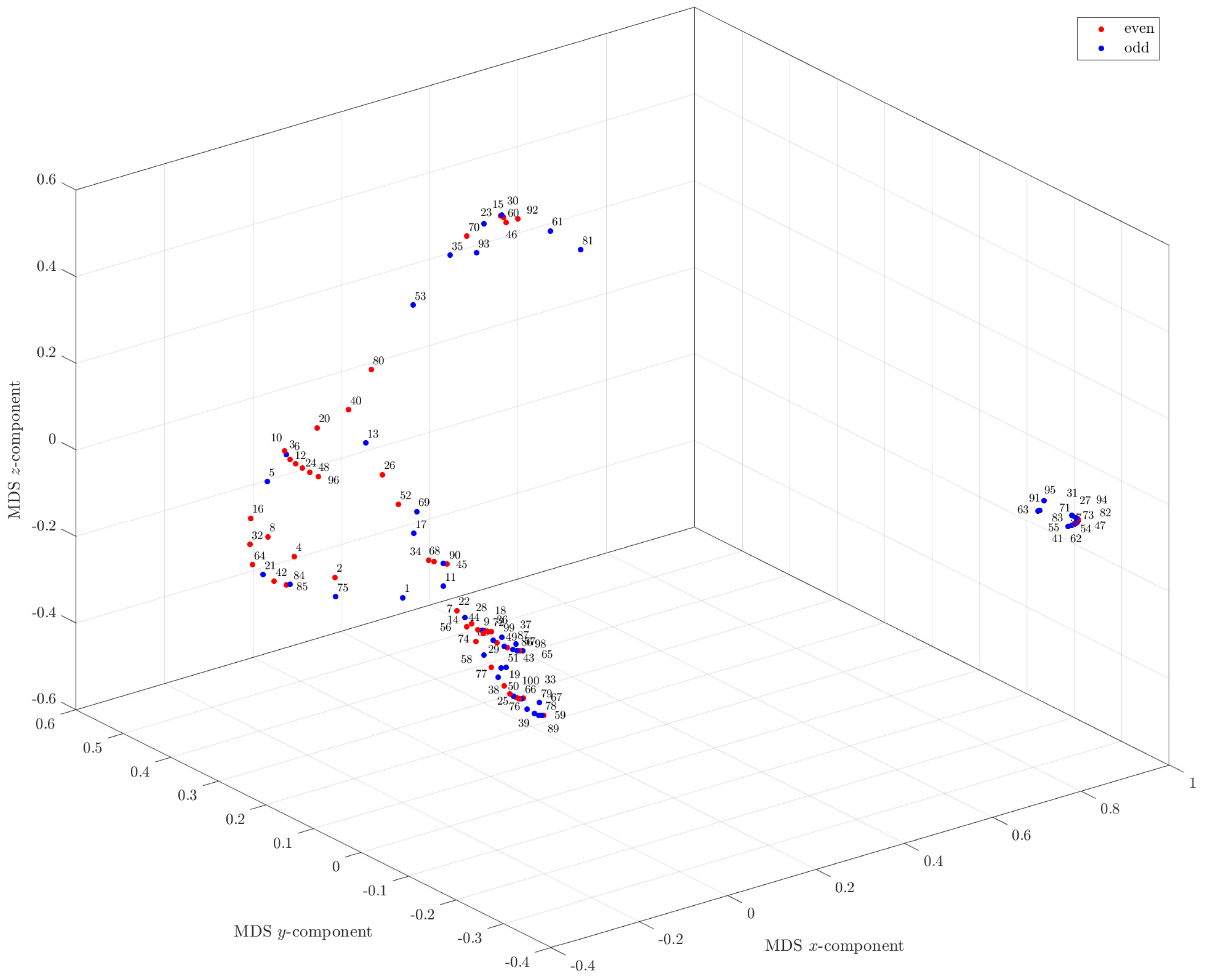
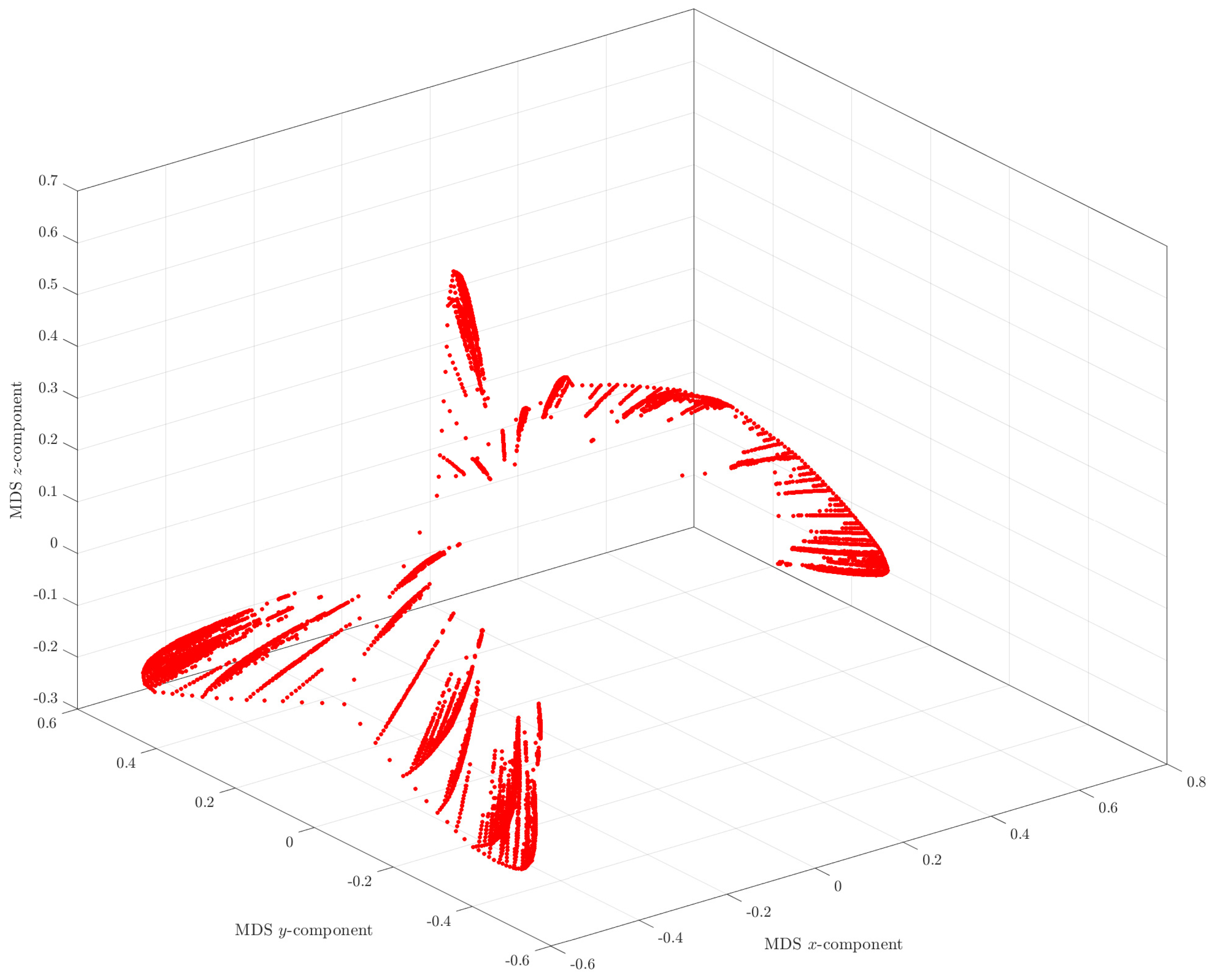
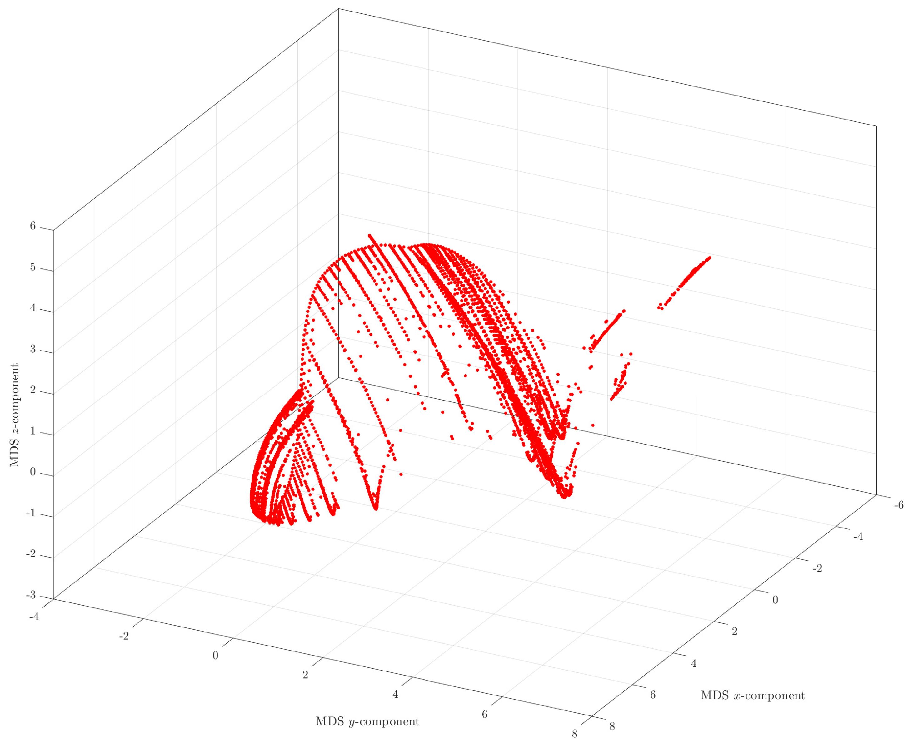
3.4. MDS Analysis of the Hailstone Sequences

We start by a limited set of numbers, which are represented by points and identified by a label corresponding to the number.

Figure 1 and Figure 2 show the dendrogram and the hierarchical tree for the first 100 numbers using the ArcCosine–Hamming distance $d_{AC}$, respectively.

Figure 3 shows the MDS three-dimensional chart for the first $N=100$ numbers using the ArcCosine–Hamming distance, where even and odd numbers are represented by blue and red marks, respectively. We observe: (i) the emergence of a clear three-dimensional structure; (ii) that even and odd numbers are not defining the ‘branches’ in the plot; and (iii) well known sequences such as $1\leftrightarrow 2\leftrightarrow 4\leftrightarrow 8\leftrightarrow 16\dots$. In a practical perspective, the point labels reduce significantly the readability and, therefore, are not considered in the follow-up for MDS plots tackling a large dataset. The Sheppard and stress plots are not represented here for the sake of parsimony and because they are of minor relevance. Nonetheless, the clustering quality of the achieved plot was confirmed.

We now test the six distances (5) for $N={10}^4$ numbers. The resulting three-dimensional MDS maps are depicted in Figure 4, Figure 5, Figure 6, Figure 7, Figure 8 and Figure 9, for the distances $d_{AC}$, $d_{Ma}$, $d_{Eu}$, $d_{Ca}$, $d_{Cl}$ and $d_{Lo}$, respectively.

The six charts are distinct since they reflect the results of different distances. Nonetheless, in all cases, we obtain clear patterns, confirming that using a three-dimensional representation reveals more clearly properties embedded in the original dataset. Moreover, from the point of view of having some kind of regular pattern, the ArcCosine–Hamming, Canberra–Hamming and Clark–Hamming distances, depicted in Figure 4, Figure 7 and Figure 8, respectively, seem more appealing. We must note that the ascetic aspects are not relevant from the point of view of the MDS interpretation. Nonetheless, as usual in MDS, the emergence of patterns and clusters for some specific distances is clearer. The full understanding of the patterns is however a more intricate problem and, in fact, no definitive conclusion was reached due to the high number of points needed to have a definitive opinion. Indeed, it was verified that more dense plots were obtained by considering a larger set of numbers, and that the many of the new points are located in the middle of the previous ones. For example, Figure 10 shows the MDS three-dimensional chart for the first $N=2\times {10}^4$ numbers using the ArcCosine–Hamming distance. The pairs of closest points are connected by means of a line. The resulting plot has four main branches, similar to what occurs in Figure 4. Nonetheless, the gaps between points are now much smaller and the lines are almost not visible. This effect is due to the presence of new points in between the previous ones, revealing a complex interaction between the ‘first’ and the ’last’ numbers.

As we mentioned above, the methods that have been exposed can be used to explore some hidden patterns in the Collatz sequence. In this sense, this exploration has shown that the orbits of the Collatz sequence exhibit a rich structure. On the one hand, it is difficult to give an interpretation of such patterns. Besides, it is almost sure that any future proof for Collatz conjecture will mainly involve high level mathematical arguments, possibly combined with computational algorithms. On the other hand, we observe that the adoption of visualization techniques may give helpful hints about the Collatz conjecture. Indeed, the difficulty in construing these patterns is what makes them a relevant topic to study, and their better interpretation can lead to developments in understanding the problem. Moreover, on another level of reasoning, we can wander if such clustering and visualization techniques can boost further progress in other problems in mathematics.

We focus on the three-dimensional MDS representations, but in good truth we can include indirectly other dimensions or information. In fact, we can change, for example, the color and/or the size of the marks according to the evolution of some additional variables. With these ideas in mind, Figure 11 shows the MDS three-dimensional chart for the first $N={10}^4$ numbers using the ArcCosine–Hamming distance $d_{AC}$, including the number information encoded by the size and color of the marks. We verify that the fundamental structure is formed by the initial numbers (in small size blue marks) and that the succeeding values (in larger yellow, orange and red marks) aggregate in the secondary branches. However, as noted above, the new points do not have a ‘monotonic’ evolution along those branches, and, instead, we note some ‘mixture’ of smaller and higher numbers.

4. Conclusions

This paper proposes a clustering perspective to analyze the Collatz conjecture. The Hailstone sequences were analyzed by means of clustering techniques, namely the HC and MDS computational algorithms. The HC leads to two-dimensional graphical representations such as dendrograms and trees. On the other hand, the MDS set of points can be visualized through two- or three-dimensional charts. The three-dimensional MDS map, in particular, reveals a complex pattern not easily observable by two-dimensional representations. A set of six distances was tested in conjunction to the Hamming-like classification. All representations revealed intricate patterns, but the ArcCosine–Hamming, Canberra–Hamming and Clark–Hamming distances in the three-dimensional MDS maps produced clearer structures. The interpretation of the results is however not straightforward, and future efforts are needed to continue with this line of research.

References

1. Lagarias, J. The Ultimate Challenge: The 3x + 1 Problem; American Mathematical Society: Providence, RI, USA, 2010. [Google Scholar]
2. Ilia Krasikov, J.C.L. Bounds for the 3x + 1 problem using difference inequalities. Acta Arith. 2003, 109, 237–258. [Google Scholar] [CrossRef] [Green Version]
3. Tao, T. Almost all orbits of the Collatz map attain almost bounded values. arXiv 2019, arXiv:1909.03562v3. [Google Scholar]
4. Eliahou, S. The 3x + 1 problem: New lower bounds on nontrivial cycle lengths. Discret. Math. 1993, 118, 45–56. [Google Scholar] [CrossRef]
5. Böhm, C.; Sontacchi, G. On the existence of cycles of given length in integer sequences like xn+1 = xn/2 if xn even, and xn+1 = 3xn + 1 otherwise. Atti Accad. Naz. Lincei VIII. Ser. Rend. Cl. Sci. Fis. Mat. Nat. 1978, 64, 260–264. [Google Scholar]
6. Andrei, S.; Kudlek, M.; Niculescu, R.S. Chains in Collatz’s Tree; Technical Report; Department of Informatics, Universität Hamburg: Hamburg, Germany, 1999. [Google Scholar]
7. Andaloro, P.J. The 3x + 1 Problem and Directed Graphs. Fibonacci Q. 2002, 40, 43–54. [Google Scholar]
8. Snapp, B.; Tracy, M. The Collatz Problem and Analogues. J. Integer Seq. 2008, 11, 1–10. [Google Scholar]
9. Laarhoven, T.; de Weger, B. The Collatz conjecture and De Bruijn graphs. Indag. Math. 2013, 24, 971–983. [Google Scholar] [CrossRef] [Green Version]
10. Emmert-Streib, F. Structural Properties and Complexity of a New Network Class: Collatz Step Graphs. PLoS ONE 2013, 8, e56461. [Google Scholar] [CrossRef] [Green Version]
11. Sultanow, E.; Koch, C.; Cox, S. Collatz Sequences in the Light of Graph Theory; Universität Potsdam: Potsdam, Germany, 2019. [Google Scholar] [CrossRef]
12. Ebert, H. A Graph Theoretical Approach to the Collatz Problem. arXiv 2020, arXiv:1905.07575. [Google Scholar]
13. Kruskal, J. Multidimensional scaling by optimizing goodness of fit to a nonmetric hypothesis. Psychometrika 1964, 29, 1–27. [Google Scholar] [CrossRef]
14. Kruskal, J.B.; Wish, M. Multidimensional Scaling; Sage Publications: Newbury Park, CA, USA, 1978. [Google Scholar]
15. Sammon, J.W. A nonlinear mapping for data structure analysis. IEEE Trans. Comput. 1969, C-18, 401–409. [Google Scholar] [CrossRef]
16. Hartigan, J.A. Clustering Algorithms; John Wiley & Sons, Inc.: Hoboken, NJ, USA, 1975. [Google Scholar]
17. Borg, I.; Groenen, P.J. Modern Multidimensional Scaling-Theory and Applications; Springer: New York, NY, USA, 2005. [Google Scholar]
18. De Leeuw, J.; Mair, P. Multidimensional scaling using majorization: Smacof in R. J. Stat. Softw. 2009, 31, 1–30. [Google Scholar] [CrossRef] [Green Version]
19. Shepard, R.N. The analysis of proximities: Multidimensional scaling with an unknown distance function. Psychometrika 1962, 27, 125–140. [Google Scholar] [CrossRef]
20. Fernández, A.; Gómez, S. Solving non-uniqueness in agglomerative hierarchical clustering using multidendrograms. J. Classif. 2008, 25, 43–65. [Google Scholar] [CrossRef] [Green Version]
21. Saeed, N.; Nam, H.; Haq, M.I.U.; Muhammad Saqib, D.B. A Survey on Multidimensional Scaling. ACM Comput. Surv. (CSUR) 2018, 51, 47. [Google Scholar] [CrossRef] [Green Version]
22. Machado, J.T.; Lopes, A. Multidimensional scaling and visualization of patterns in prime numbers. Commun. Nonlinea. Sci. Numer. Simul. 2020, 83, 105128. [Google Scholar] [CrossRef]
23. Machado, J.A.T. An Evolutionary Perspective of Virus Propagation. Mathematics 2020, 8, 779. [Google Scholar] [CrossRef]
24. Machado, J.T.; Lopes, A.M. A computational perspective of the periodic table of elements. Commun. Nonlinea. Sci. Numer. Simul. 2019, 78, 104883. [Google Scholar] [CrossRef]
25. Machado, J.T.; Lopes, A.M. Multidimensional scaling locus of memristor and fractional order elements. J. Adv. Res. 2020, 25, 147–157. [Google Scholar] [CrossRef]
26. Machado, J.A.T.; Rocha-Neves, J.M.; Andrade, J.P. Computational analysis of the SARS-CoV-2 and other viruses based on the Kolmogorov’s complexity and Shannon’s information theories. Nonlinear Dyn. 2020, 101, 1731–1750. [Google Scholar] [CrossRef]
27. Tenreiro Machado, J.A.; Lopes, A.M.; Galhano, A.M. Multidimensional Scaling Visualization Using Parametric Similarity Indices. Entropy 2015, 17, 1775–1794. [Google Scholar] [CrossRef] [Green Version]
28. Aggarwal, C.C.; Hinneburg, A.; Keim, D.A. On the Surprising Behavior of Distance Metrics in Gigh Dimensional Space; Springer: Berlin/Heidelberg, Germany, 2001. [Google Scholar]
29. Sokal, R.R.; Rohlf, F.J. The comparison of dendrograms by objective methods. Taxon 1962, 33–40. [Google Scholar] [CrossRef]
30. Felsenstein, J. PHYLIP (Phylogeny Inference Package), Version 3.5 c; University of Washington: Seattle, WA, USA, 1993. [Google Scholar]
31. Tuimala, J. A Primer to Phylogenetic Analysis Using the PHYLIP Package; CSC—Scientific Computing Ltd.: Leeds, UK, 2006. [Google Scholar]
32. Cha, S.H. Comprehensive Survey on Distance/Similarity Measures between Probability Density Functions. Int. J. Math. Models Methods Appl. Sci. 2007, 1, 300–307. [Google Scholar]
33. Deza, M.M.; Deza, E. Encyclopedia of Distances; Springer-Verlag: Berlin, Heidelberg, 2009. [Google Scholar]
34. Hamming, R.W. Error Detecting and Error Correcting Codes. Bell Syst. Tech. J. 1950, 29, 147–160. [Google Scholar] [CrossRef]
Figure 1. The dendrogram for the first 100 numbers using the ArcCosine–Hamming distance d A C .
Mathematics 09 00314 g001
Figure 2. The hierarchical tree for the first 100 numbers using the ArcCosine–Hamming distance d A C .
Mathematics 09 00314 g002
Figure 3. The MDS three-dimensional chart for the first N = 100 numbers using the ArcCosine–Hamming distance d A C .
Mathematics 09 00314 g003
Figure 4. The MDS three-dimensional chart for the first N = 10 4 numbers using the ArcCosine–Hamming distance d A C .
Mathematics 09 00314 g004
Figure 5. The MDS three-dimensional chart for the first N = 10 4 numbers using the Manhattan–Hamming distance d M a .
Mathematics 09 00314 g005
Figure 6. The MDS three-dimensional chart for the first N = 10 4 numbers using the Euclidean–Hamming distance d E u .
Mathematics 09 00314 g006
Figure 7. The MDS three-dimensional chart for the first N = 10 4 numbers using the Canberra–Hamming distance d C a .
Mathematics 09 00314 g007
Figure 8. The MDS three-dimensional chart for the first N = 10 4 numbers using the Clark–Hamming distance d C l .
Mathematics 09 00314 g008
Figure 9. The MDS three-dimensional chart for the first N = 10 4 numbers using the Lorentzian–Hamming distance d L o .
Mathematics 09 00314 g009
Figure 10. The MDS three-dimensional chart for the first N = 2 × 10 4 numbers using the ArcCosine–Hamming distance d A C .
Mathematics 09 00314 g010
Figure 11. The MDS three-dimensional chart for the first N = 2 × 10 4 numbers using the ArcCosine–Hamming distance d A C . The size and color of the marks are proportional to the numbers.
Mathematics 09 00314 g011
Publisher’s Note: MDPI stays neutral with regard to jurisdictional claims in published maps and institutional affiliations.