Reliable Efficient Difference Methods for Random Heterogeneous Diffusion Reaction Models with a Finite Degree of Randomness

Abstract

This paper deals with the search for reliable efficient finite difference methods for the numerical solution of random heterogeneous diffusion reaction models with a finite degree of randomness. Efficiency appeals to the computational challenge in the random framework that requires not only the approximating stochastic process solution but also its expectation and variance. After studying positivity and conditional random mean square stability, the computation of the expectation and variance of the approximating stochastic process is not performed directly but through using a set of sampling finite difference schemes coming out by taking realizations of the random scheme and using Monte Carlo technique. Thus, the storage accumulation of symbolic expressions collapsing the approach is avoided keeping reliability. Results are simulated and a procedure for the numerical computation is given.

1. Introduction

Dealing with deterministic partial differential equations (PDE), finite difference methods (FD) are probably the most used because they are easy to apply and fairly efficient,  [1,2]. Trying to capture real world problems, the models introduced uncertainty in several ways, basically assuming that both data, parameters, initial and or boundary conditions are stochastic processes instead of deterministic functions, [3,4]. The uncertainty appears not only because of error measurements, but also considering heterogeneity of the media, material impurities, or even the lack of access to measurements  [5,6]. Independently of the type of modelling the uncertainty, the consideration of partial differential equations models (PDEM) has particular challenges. In fact, it is necessary to compute not only the stochastic process solution or approximating stochastic process, but also their statistical moments, mainly the expectation and the variance. Integral transforms methods are efficient techniques to solve PDEM based on integration resources in fitting domains [7,8]. Another powerful technique suitable for models with complex geometries is the finite element method [9]. Iterative methods, for instance FD have particular troubles derived from the storage accumulation of intermediate levels when the computer manages symbolically the involved stochastic processes, [10,11,12]. This drawback of the iterative methods for solving PDEM occurs in both approaches, the one based on Itô calculus [13] the so-called stochastic differential approach (SDEA), as well as the one based on the mean square calculus  [14] also called random differential equations approach (RDEA). To face this computational challenge we take a set of realizations of the model, then we solve each sampled problem using FD method. Finally, we use Monte Carlo technique, [15,16] to average the results of the deterministic sampled problems to compute the expectation and the variance of the approximating solution stochastic process. In our model the involved stochastic processes (s.p.’s) are defined in a complete probability space $(\mathsf{\Omega },\mathcal{F},\mathbb{P})$ and have n degrees of randomness [14] (p. 37), i.e., they only depend on a finite number n of random variables (r.v.’s):

$$\begin{array}{c}\hfill h\left(s\right)=F(s,A_1,A_2,\dots ,A_n),\end{array}$$

(1)

where

$$\begin{array}{c}\hfill \left.\begin{array}{c}\hfill A_i,i=1,\dots ,n,\mathrm{are}\mathrm{mutually}\mathrm{independent}\mathrm{r}.\mathrm{v}.’\mathrm{s};\\ \\ \hfill F\mathrm{is}\mathrm{a}\mathrm{differentiable}\mathrm{real}\mathrm{function}\mathrm{of}\mathrm{the}\mathrm{variable}s\\ \hfill (\mathrm{being}s\mathrm{the}\mathrm{spatial}\mathrm{variable}x\mathrm{or}\mathrm{the}\mathrm{temporal}\mathrm{one}t).\end{array}\right\}\end{array}$$

(2)

In addition, under this hypothesis, the s.p. $h\left(s\right)$ has sample differentiable trajectories (realizations), i.e., for a fixed event $\omega \in \mathsf{\Omega }$, the real function $h(s,\omega )=F(s,A_1\left(\omega \right),A_2\left(\omega \right),\dots ,A_n\left(\omega \right))$ is a differentiable function of the real variable s. For the sake of clarity in the presentation and to save notational complexity, we will assume that involved s.p.’s in the coefficients and initial or boundary conditions, have one degree of randomness, i.e., they have the form

$$\begin{array}{c}\hfill h\left(s\right)=F(s,A),\end{array}$$

with A a r.v. and F a differentiable real function of the variable s. Then the s.p. $h\left(s\right)$ has sample differentiable trajectories, i.e., for a fixed event $\omega \in \mathsf{\Omega }$, the real function $h(s,\omega )=F(s,A(\omega \left)\right)$ is a differentiable function of the real variable s.

This paper deals with random parabolic partial differential models of the form

$$\begin{array}{ccc}\hfill \frac{\mathsf{\partial }u(x,t)}{\mathsf{\partial }t}& =& \frac{\mathsf{\partial }}{\mathsf{\partial }x}\left[p\left(x\right){\displaystyle \frac{\mathsf{\partial }u(x,t)}{\mathsf{\partial }x}}\right]-q\left(x\right)u(x,t),0<x<1,t>0,\hfill \end{array}$$

(3)

$$\begin{array}{ccc}\hfill u(0,t)& =& g_1\left(t\right),t>0,\hfill \end{array}$$

(4)

$$\begin{array}{ccc}\hfill u(1,t)& =& g_2\left(t\right),t>0,\hfill \end{array}$$

(5)

$$\begin{array}{ccc}\hfill u(x,0)& =& f\left(x\right),0\le x\le 1,\hfill \end{array}$$

(6)

where the diffusion coefficient $p\left(x\right)$, the reaction coefficient $q\left(x\right)$, the boundary conditions $g_i\left(t\right)$, $i=1,2$, and the initial condition $f\left(x\right)$ are s.p.’s with one degree of randomness in the sense as defined above. In addition we assume that $p\left(x\right)$, $q\left(x\right)$, $f\left(x\right)$ and $g_i\left(t\right)$, $i=1,2$ are mean square continuous s.p.’s in variables x and t, respectively, $p\left(x\right)$ is also a mean square differentiable s.p. and the sample realizations of the random inputs $p\left(x\right)$, $q\left(x\right)$, $g_i\left(t\right)$, $i=1,2$ and $f\left(x\right)$ satisfy the following conditions denoting $p^{\prime }\left(x\right)$ as the mean square derivative of $p\left(x\right)$:

$$\begin{array}{cc}\hfill 0<a_1\le p(x,\omega )\le a_2<+\mathsf{\infty },& x\in [0,1],\mathrm{for}\mathrm{almost}\mathrm{every}(\mathrm{a}.\mathrm{e}.)\omega \in \mathsf{\Omega },\end{array}$$

(7)

$$\begin{array}{cc}\hfill {\displaystyle \frac{|p^{\prime }(x,\omega )|}{p(x,\omega )}}\le b<+\mathsf{\infty },& x\in [0,1],\mathrm{for}\mathrm{a}.\mathrm{e}.\omega \in \mathsf{\Omega },\end{array}$$

(8)

$$\begin{array}{cc}\hfill q_{\min }\le q(x,\omega )\le q_{\max },& x\in [0,1],\mathrm{for}\mathrm{a}.\mathrm{e}.\omega \in \mathsf{\Omega },\end{array}$$

(9)

$$\begin{array}{cc}\hfill g_i(t,\omega )\ge 0,i=1,2,& t>0,\mathrm{for}\mathrm{a}.\mathrm{e}.\omega \in \mathsf{\Omega },\end{array}$$

(10)

$$\begin{array}{cc}\hfill 0\le f(x,\omega )\le f_{\max },& x\in [0,1],\mathrm{for}\mathrm{a}.\mathrm{e}.\omega \in \mathsf{\Omega },\end{array}$$

(11)

This model is frequent in chemical engineering sciences and in heat and mass transfer theory for reaction-diffusion problems with parameters depending on the spatial variables as it occurs in heterogeneous and anisotropic solids, [17] (p. 455), [18] (p. 388), [19,20].

The paper is organized as follows. Section 2 deals with some preliminaries, definitions and notations about the mean square calculus as well as the construction of the random mean square finite difference scheme (RMSFDS) resulting from the discretization of model (3)–(6). Section 3 is addressed to the study of properties of the RMSFDS such as positivity, stability and consistency. Throughout a sample approach, sufficient conditions for stability and positivity of the random numerical solution s.p. in terms of the data and discretization step-sizes are found. Consistency of the RMSFDS with Equation (3) is also treated throughout a sample approach and the consistency of the corresponding realized deterministic scheme for each fixed event $\omega \in \mathsf{\Omega }$. In Section 4 we construct an algorithm to perform the efficient computation of the expectation and the variance of the numerical solution s.p. using Monte Carlo method and the solution of the sampled scheme. Numerical simulations for a problem where the exact solution is known are performed showing the efficiency of the proposed numerical method as well as the computations of the expectation and the variance of the numerical approximated s.p. A conclusion Section 5 ends the paper.

2. Preliminaries and Construction of the Random Finite Difference Scheme

For the sake of clarity in the presentation, in this section we recall some definitions and concepts related to the $L_p$-calculus, [14]. In a probability space $\left(\mathsf{\Omega },\mathcal{F},\mathcal{P}\right)$, we denote $L_p\left(\mathsf{\Omega }\right)$ the space of all real valued r.v.’s $U:\mathsf{\Omega }\to \mathbb{R}$ of order p, endowed with the norm

$${\parallel U\parallel }_p={\left(\mathbb{E}\left[\right|U{|}^p]\right)}^{1/p}={\left({\int }_{\mathsf{\Omega }}{\left|U\left(\omega \right)\right|}^p{f}_U\left(\omega \right)\mathrm{d}\omega \right)}^{1/p}<+\mathsf{\infty },$$

(12)

where $\mathbb{E}[·]$ denotes the expectation operator, $f_U$ the density function of the r.v. U and $\omega$ an event of sample space $\mathsf{\Omega }$.

Given $T\subset \mathbb{R}$, a family of t-indexed r.v.’s, say $\left\{V\left(t\right):t\in T\right\}$, is called a stochastic process of order p (p-s.p.) if for each $t\in T$ fixed, the r.v. $V\left(t\right)\in L_p\left(\mathsf{\Omega }\right)$. We say that a p-s.p. $\left\{V\left(t\right):t\in T\right\}$ is p-th mean continuous at $t\in T$, if

$${\parallel V(t+h)-V\left(t\right)\parallel }_p\to 0\mathrm{as}h\to 0,t,t+h\in T.$$

Furthermore, if there exists a p-s.p. $V^{\prime }\left(t\right)$, such that

$${∥\frac{V(t+h)-V\left(t\right)}{h}-V^{\prime }\left(t\right)∥}_p\to 0\mathrm{as}h\to 0,t,t+h\in T,$$

then we say that the s.p. $\left\{V\left(t\right):t\in T\right\}$ is $p$-th mean differentiable at $t\in T$ and $V^{\prime }\left(t\right)$ is the p-derivative of $V\left(t\right)$. In the particular case that $p=2$, $L_2\left(\mathsf{\Omega }\right)$, definitions above leads to the corresponding concept of mean square (m.s.) continuity and m.s. differentiability, respectively.

In this section, we construct an explicit random finite difference scheme for solving problem (3)–(6). Firstly, let us write Equation (3) into the following form

$$\frac{\mathsf{\partial }u(x,t)}{\mathsf{\partial }t}=p\left(x\right)\frac{{\mathsf{\partial }}^{2}u(x,t)}{\mathsf{\partial }{x}^2}+p^{\prime }\left(x\right)\frac{\mathsf{\partial }u(x,t)}{\mathsf{\partial }x}-q\left(x\right)u(x,t),$$

(13)

where $p\left(x\right)\in L_p\left(\mathsf{\Omega }\right)$ is p-th mean continuous and differentiable, $p^{\prime }\left(x\right)$ is the p-derivative of $p\left(t\right)$ and $q\left(x\right)\in L_p\left(\mathsf{\Omega }\right)$ is p-th mean continuous.

Let us consider the uniform partition of the spatial interval $[0,1]$, of the form $x_i=ih$, $0\le i\le M$, with $Mh=1$. For a fixed time horizon, T, we consider $N+1$ time levels $t^n=nk$, $0\le n\le N$ with $Nk=T$. The numerical approximation of the solution s.p. of the random problem (3)–(6) is denoted by $u_i^n$, i.e.,

$$u_i^n\approx u(x_i,t^n),0\le i\le M,0\le n\le N.$$

(14)

By using a forward first-order approximation of the time partial derivative and centred second-order approximations for the spatial partial derivatives in Equation (13) one gets the following random numerical scheme for the spatial internal mesh points

$$\begin{array}{c}\hfill \frac{u_i^{n+1}-u_i^n}{k}=p_i\frac{u_{i-1}^n-2u_i^n+u_{i+1}^n}{h^2}+p_i^{\prime }\frac{u_{i+1}^n-u_{i-1}^n}{2h}-q_i{u}_i^n,1\le i\le M-1,0\le n\le N-1,\end{array}$$

(15)

where $p_i=p\left(x_i\right)$, $p_i^{\prime }=p^{\prime }\left(x_i\right)$ and $q_i=q\left(x_i\right)$. The resulting random discretized problem (3)–(6) can be rewritten in the following form

$$\begin{array}{c}\hfill \left.\begin{array}{c}\hfill u_i^{n+1}={\displaystyle \frac{k}{h^2}}\left(p_i-{\displaystyle \frac{h}{2}}{p}_i^{\prime }\right)u_{i-1}^n+\left(1-k{q}_i-{\displaystyle \frac{2k}{h^2}}{p}_i\right)u_i^n+{\displaystyle \frac{k}{h^2}}\left(p_i+{\displaystyle \frac{h}{2}}{p}_i^{\prime }\right)u_{i+1}^n,\\ \hfill 1\le i\le M-1,1\le n\le N-1,\\ \\ \hfill u_0^n=g_1^n,u_M^n=g_2^n,1\le n\le N,\\ \\ \hfill u_i^0=f_i,0\le i\le M,\end{array}\right\}\end{array}$$

(16)

where $g_1^n=g_1\left(t^n\right)$, $g_2^n=g_2\left(t^n\right)$, and $f_i=f\left(x_i\right)$. Please note that all the inputs of the random problem (16) are s.p.’s depending on one finite degree of randomness and lie in $L_p\left(\mathsf{\Omega }\right)$.

3. Properties of the Random Numerical Scheme: Positivity, Stability and Consistency

We are going to prove the positivity of the random numerical solution $\left\{u_i^n,0\le i\le M\right.$, $\left.0\le n\le N\right\}$ of the random scheme (16) and its ${\parallel ·\parallel }_p$-stability in the sense of fixed station respect to the time. We extend this type of stability to the random field.

Definition 1.

A random numerical scheme is said to be ${\parallel ·\parallel }_p$-stable in the fixed station sense in the domain $[0,1]\times [0,T]$, if for every partition with $k=\mathsf{\Delta }t$, $h=\mathsf{\Delta }x$ such that $Nk=T$ and $Mh=1$,

$$\parallel u_i^n{\parallel }_p\le C,0\le i\le M,0\le n\le N,$$

(17)

where C is independent of the step-sizes h, k and the time level n.

First, we are going to find sufficient conditions on the spatial step-size h and the temporal step-size k, so that the numerical solution $\left\{u_i^n\left(\omega \right)\right\}$ constructed by sampling random scheme (16) for a fixed $\omega \in \mathsf{\Omega }$

$$\begin{array}{c}\hfill \left.\begin{array}{c}\hfill u_i^{n+1}\left(\omega \right)=\\ \hfill {\displaystyle \frac{k}{h^2}}\left(p_i\left(\omega \right)-{\displaystyle \frac{h}{2}}{p}_i^{\prime }\left(\omega \right)\right)u_{i-1}^n+\left(1-k{q}_i\left(\omega \right)-{\displaystyle \frac{2k}{h^2}}{p}_i\left(\omega \right)\right)u_i^n+{\displaystyle \frac{k}{h^2}}\left(p_i\left(\omega \right)+{\displaystyle \frac{h}{2}}{p}_i^{\prime }\left(\omega \right)\right)u_{i+1}^n,\\ \hfill 1\le i\le M-1,1\le n\le N-1,\\ \\ \hfill u_0^n\left(\omega \right)=g_1^n\left(\omega \right),u_M^n\left(\omega \right)=g_2^n\left(\omega \right),1\le n\le N,\\ \\ \hfill u_i^0\left(\omega \right)=f_i\left(\omega \right),0\le i\le M,\end{array}\right\}\end{array}$$

(18)

guarantee its positivity, i.e., $u_i^n\left(\omega \right)\ge 0$ for $0\le i\le M$ and for each time level n, $0\le n\le N$. We denote

$$\begin{array}{c}\hfill \begin{array}{ccc}\hfill A_i(h,k)\left(\omega \right)& =& {\displaystyle \frac{k}{h^2}}\left(p_i\left(\omega \right)-{\displaystyle \frac{h}{2}}{p}_i^{\prime }\left(\omega \right)\right),\hfill \\ \hfill B_i(h,k)\left(\omega \right)& =& 1-k{q}_i\left(\omega \right)-{\displaystyle \frac{2k}{h^2}}{p}_i\left(\omega \right),\hfill \\ \hfill C_i(h,k)\left(\omega \right)& =& p_i\left(\omega \right)+{\displaystyle \frac{h}{2}}{p}_i^{\prime }\left(\omega \right),\hfill \end{array}\end{array}$$

(19)

then the sampling scheme (18) can be rewritten as follows

$$u_i^{n+1}\left(\omega \right)=A_i(h,k)\left(\omega \right)u_{i-1}^n\left(\omega \right)+B_i(h,k)\left(\omega \right)u_i^n\left(\omega \right)+C_i(h,k)\left(\omega \right)u_{i+1}^n\left(\omega \right).$$

To guarantee the positivity of the numerical approximation $\left\{u_i^n\left(\omega \right)\right\}$ it is sufficient to impose the positivity of coefficients defined in (19). Please note that the simultaneously positivity of coefficients $A_i(h,k)\left(\omega \right)$ and $C_i(h,k)\left(\omega \right)$ means that

$$-p_i\left(\omega \right)\le {\displaystyle \frac{h}{2}}{p}_i^{\prime }\left(\omega \right)\le p_i\left(\omega \right),$$

that is

$$h\le {\displaystyle \frac{2p_i\left(\omega \right)}{|p_i^{\prime }\left(\omega \right)|}}.$$

(20)

Taking into account the bound condition (8) it follows that coefficients $A_i(h,k)\left(\omega \right)$ and $C_i(h,k)\left(\omega \right)$, $1\le i\le M-1$, are non-negative for a.e. $\omega \in \mathsf{\Omega }$ under condition

$$h\le {\displaystyle \frac{2}{b}}.$$

(21)

Please note that for the particular case where $p_i\left(\omega \right)$ is constant the positivity of coefficients $A_i(h,k)\left(\omega \right)$ and $C_i(h,k)\left(\omega \right)$ defined in (19), is established for $h>0$. To guarantee the positivity of coefficient $B_i(h,k)\left(\omega \right)$ from (19) and bounds (7)–(9) note that

$$B_i(h,k)\left(\omega \right)=1-k{q}_i\left(\omega \right)-\frac{2k}{h^2}{p}_i\left(\omega \right)\ge 1-k{q}_{\max }-\frac{2k}{h^2}{a}_2.$$

(22)

Thus, the positivity of $B_i(h,k)\left(\omega \right)$, $1\le i\le M-1$, for a.e. $\omega \in \mathsf{\Omega }$, is verified under the conditions

$$\begin{array}{ccc}\hfill k\le \frac{h^2}{2a_2},& & (\mathrm{If}{q}_{\max }<0),\hfill \end{array}$$

(23)

$$\begin{array}{ccc}\hfill k\le \frac{h^2}{2a_2+h^2{q}_{\max }},& & (\mathrm{If}{q}_{\max }\ge 0).\hfill \end{array}$$

(24)

Then taking into account the sufficient conditions (21), (23) and (24) over the discretization step-sizes h and k, the positivity of all the coefficients (19) of sampling scheme (18) for a.e. $\omega \in \mathsf{\Omega }$ is guaranteed and consequently the positivity of the numerical solution $\left\{u_i^n\left(\omega \right)\right\}$, $0\le i\le M$, for each time level n, $0\le n\le N$, $(T=kN)$ is established.

Let us prove now that random numerical scheme (16) is ${\parallel ·\parallel }_p$-stable in the sense of Definition 1. In this study we need to distinguish two cases for the sampling parameter $q_i\left(\omega \right)$ for a fixed $\omega \in \mathsf{\Omega }$.

Case 1.

$\boxed{q_i\left(\omega \right)\ge 0}$, $0\le i\le M$.

From (18) imposing conditions (21) and (24) one gets

$$\begin{array}{ccc}\hfill u_i^{n+1}\left(\omega \right)& \le & \left(A_i(h,k)\left(\omega \right)+B_i(h,k)\left(\omega \right)+C_i(h,k)\left(\omega \right)\right)u_{{\mathrm{MAX}}_i}^n\left(\omega \right)\hfill \\ & \le & \left(1-k{q}_i\left(\omega \right)\right)u_{{\mathrm{MAX}}_i}^n\left(\omega \right)\hfill \\ & \le & u_{{\mathrm{MAX}}_i}^n\left(\omega \right),1\le i\le M-1,0\le n\le N-1,\hfill \end{array}$$

(25)

where

$$u_{{\mathrm{MAX}}_i}^n\left(\omega \right)=\underset{0\le i\le M}{max}\left\{u_i^n\left(\omega \right)\right\}.$$

(26)

Using (11), the boundary conditions of (18) and (25) we have by recurrence

$$\begin{array}{ccc}\hfill u_i^{n+1}\left(\omega \right)& \le & max\{g_1^{n+1}\left(\omega \right),g_2^{n+1}\left(\omega \right),u_{{\mathrm{MAX}}_i}^n\left(\omega \right)\}\hfill \\ & \le & max\{g_1^{n+1}\left(\omega \right),g_2^{n+1}\left(\omega \right),g_1^n\left(\omega \right),g_2^n\left(\omega \right),u_{{\mathrm{MAX}}_i}^{n-1}\left(\omega \right)\}\hfill \\ & \le & \cdots \hfill \\ & \le & \underset{1\le s\le n+1}{max}\left\{g_1^s\left(\omega \right),g_2^s\left(\omega \right),u_{{\mathrm{MAX}}_i}^0\left(\omega \right)\right\}\hfill \\ & \le & \underset{0\le t\le (n+1)k}{max}\left\{g_1(t,\omega ),g_2(t,\omega ),\underset{x\in [0,1]}{max}\left\{f(x,\omega )\right\}\right\}.\hfill \end{array}$$

(27)

We denote

$$G\left(T\right)=\underset{0\le t\le T}{max}\left\{g_{1,\max }\left(T\right),g_{2,\max }\left(T\right),f_{\max }\right\},$$

(28)

where

$$g_{i,\max }\left(T\right)=\underset{0\le t\le T}{max}\{g_i(t,\omega ),\mathrm{for}\mathrm{a}.\mathrm{e}.\omega \in \mathsf{\Omega }\},i=1,2.$$

(29)

Thus, from (27) and (28) we obtain the following upper bound for the numerical solution of sampling scheme (18)

$$0\le u_i^n\left(\omega \right)\le G\left(T\right),\mathrm{for}\mathrm{a}.\mathrm{e}.\omega \in \mathsf{\Omega },$$

(30)

for each level n, $0\le n\le N=Tk$, and for each spatial point $x_i$, $0\le i\le M$.

Case 2.

$\boxed{q_{\min }\le {min}_{0\le i\le M}\left\{q_i\left(\omega \right)\right\}<0}$

From (18) imposing conditions (21) and (23) and using (25) and (26) we obtain

$$\begin{array}{ccc}\hfill u_i^{n+1}\left(\omega \right)& \le & \left(1-k{q}_i\left(\omega \right)\right)u_{{\mathrm{MAX}}_i}^n\left(\omega \right)\hfill \\ & \le & \left(1+k|q_{\min }|\right)u_{{\mathrm{MAX}}_i}^n\left(\omega \right),1\le i\le M-1,0\le n\le N-1.\hfill \end{array}$$

(31)

Then using the boundary conditions of (18) and applying recurrently the bound exhibits in (31) one gets

$$\begin{array}{ccc}\hfill u_i^{n+1}\left(\omega \right)& \le & max\{g_1^{n+1}\left(\omega \right),g_2^{n+1}\left(\omega \right),\left(1+k|q_{\min }|\right)u_{{\mathrm{MAX}}_i}^n\left(\omega \right)\}\hfill \\ & \le & max\{g_1^{n+1}\left(\omega \right),g_2^{n+1}\left(\omega \right),\left(1+k|q_{\min }|\right)max\{g_1^n\left(\omega \right),g_2^n\left(\omega \right),\left(1+k|q_{\min }|\right)u_{{\mathrm{MAX}}_i}^{n-1}\left(\omega \right)\}\hfill \\ & \le & {\left(1+k|q_{\min }|\right)}^{2}max\{g_1^{n+1}\left(\omega \right),g_2^{n+1}\left(\omega \right),g_1^n\left(\omega \right),g_2^n\left(\omega \right),u_{{\mathrm{MAX}}_i}^{n-1}\left(\omega \right)\}\hfill \\ & \le & \cdots \hfill \\ & \le & {\left(1+k|q_{\min }|\right)}^{n+1}\underset{1\le s\le n+1}{max}\left\{g_1^s\left(\omega \right),g_2^s\left(\omega \right),u_{{\mathrm{MAX}}_i}^0\left(\omega \right)\right\}.\hfill \end{array}$$

(32)

Taking into account the following inequality

$${\left(1+k|q_{\min }|\right)}^s\le {\left(1+k|q_{\min }|\right)}^N<{\mathrm{e}}^{T|q_{\min }|},0\le s\le N,$$

and the notation introduced in (28), we obtain this upper bound for the numerical solution of sample scheme (18)

$$0\le u_i^n\left(\omega \right)\le {\mathrm{e}}^{T|q_{\min }|}G\left(T\right),\mathrm{for}\mathrm{a}.\mathrm{e}.\omega \in \mathsf{\Omega },$$

(33)

for each level n, $0\le n\le N=Tk$, and for each spatial point $x_i$, $0\le i\le M$.

Please note that both bounds (30) and (33) are independent of n, h and k.

Finally, under discretization step-size conditions (21), (23) and (24) and from the upper bounds (30) and (33) it follows that

$$\begin{array}{c}\hfill \parallel u_i^n{\parallel }_p={\left(\mathbb{E}\left[{\left|u_i^n\right|}^p\right]\right)}^{1/p}={\left({\int }_{\mathsf{\Omega }}{\left|u_i^n\left(\omega \right)\right|}^p{f}_{u_i^n}\left(\omega \right)\mathrm{d}\omega \right)}^{1/p}\le \alpha \left(T\right)G\left(T\right)\underset{1}{\underbrace{{\left({\int }_{\mathsf{\Omega }}{f}_{u_i^n}\left(\omega \right)\mathrm{d}\omega \right)}^{1/p}}},\end{array}$$

(34)

where $G\left(T\right)$ is defined in (28) and (29) and

$$\begin{array}{c}\hfill \alpha \left(T\right)=\left\{\begin{array}{ccc}1\hfill & \mathrm{if}& q_{\min }\ge 0,\hfill \\ {\mathrm{e}}^{T|q_{\min }|}\hfill & \mathrm{if}& q_{\min }<0.\hfill \end{array}\right.\end{array}$$

(35)

Consequently, random numerical scheme (16) is ${\parallel ·\parallel }_p$-stable in the sense of Definition 1.

Summarizing, the following result was established.

Theorem 1.

With the previous notation under conditions (21), (23) and (24) on the discretized step-sizes $h=\mathsf{\Delta }x$ and $k=\mathsf{\Delta }t$, the random numerical solution s.p. $\left\{u_i^n\right\}$ of the RMSFDS (16) for the random partial differential model (3)–(11) is positive for $0\le i\le M$ at each time-level $0\le n\le N$ with $T=kN$. Furthermore the RMSFDS (16) is ${\parallel ·\parallel }_p$-stable in the fixed station sense taking the value

$$C=\alpha \left(T\right)G\left(T\right),$$

where constants $G\left(T\right)$ and $\alpha \left(T\right)$ are defined in (28) and (35), respectively.

To prove the consistency of the random finite difference scheme (16) with the random partial differential Equation (13) let us introduce the following definition inspired in the well-known concept of consistency for deterministic PDEs, see [2].

Definition 2.

Let us consider a RMSFDS $F\left(u_i^n\right)=0$ for a random partial differential equation (RPDE) $\mathcal{L}\left(u\right)=0$ and let the local truncation error $T_i^n\left(U\left(\omega \right)\right)$ for a fixed event $\omega \in \mathsf{\Omega }$ be defined by

$$T_i^n\left(U\left(\omega \right)\right)=F\left(U_i^n\left(\omega \right)\right)-\mathcal{L}\left(U_i^n\left(\omega \right)\right),$$

where $U_i^n\left(\omega \right)$ denotes the theoretical solution of $\mathcal{L}\left(u\right)\left(\omega \right)=0$ evaluated at $(x_i,t^n)$. We call $T_i^n\left(U\right)$ by

$$\parallel T_i^n{\left(U\right)\parallel }_p={\left(\mathbb{E}\left[{\left|T_i^n\left(U\right)\right|}^p\right]\right)}^{1/p}={\left({\int }_{\mathsf{\Omega }}{\left|T_i^n\left(U\left(\omega \right)\right)\right|}^p{f}_{T_i^n\left(U\right)}\left(\omega \right)\mathrm{d}\omega \right)}^{1/p}.$$

With previous notation, the RMSFDS $F\left(u_i^n\right)=0$ is said to be ${\parallel ·\parallel }_p$-consistent with the RPDE $\mathcal{L}\left(u\right)=0$ if

$$\parallel T_i^n{\left(U\right)\parallel }_p\to 0\mathrm{as}h=▵x\to 0,k=▵t\to 0.$$

Next result shows the consistency in the p-norm of RFDS (16) with RPDE (13).

Theorem 2.

The RFDS (16) is ${\parallel ·\parallel }_p$- consistent with the RPDE (13).

Proof. 

Please note that for each fixed $\omega \in \mathsf{\Omega }$ the local truncation error using (13) and (15) is given by

$$\begin{array}{c}{T}_i^n\left(U\left(\omega \right)\right)=\frac{U_i^{n+1}\left(\omega \right)-U_i^n\left(\omega \right)}{k}-\frac{\mathsf{\partial }U\left(\omega \right)}{\mathsf{\partial }t}(x_i,t^n)-p_i\frac{U_{i-1}^n\left(\omega \right)-2U_i^n\left(\omega \right)+U_{i+1}^n\left(\omega \right)}{h^2}+\hfill \\ \hfill p_i\frac{{\mathsf{\partial }}^{2}U\left(\omega \right)}{\mathsf{\partial }{x}^2}(x_i,t^n)-p_i^{\prime }\frac{U_{i+1}^n\left(\omega \right)-U_{i-1}^n\left(\omega \right)}{2h}+p_i^{\prime }\frac{\mathsf{\partial }U\left(\omega \right)}{\mathsf{\partial }x}(x_i,t^n).\end{array}$$

Assuming that $U(x,t)\left(\omega \right)$ is four times continuously differentiable with respect to x and two times continuously differentiable with respect to t and using Taylor expansions of $U(x,t)\left(\omega \right)$ at $(x_i,t^n)$ one gets

$$T_i^n\left(U\left(\omega \right)\right)=\frac{k}{2}\frac{{\mathsf{\partial }}^{2}U\left(\omega \right)}{\mathsf{\partial }{t}^2}(x_i,\delta )-p_i\frac{h^2}{12}\frac{{\mathsf{\partial }}^{4}U\left(\omega \right)}{\mathsf{\partial }{x}^4}({\eta }_1,t^n)-p_i^{\prime }\frac{h^2}{6}\frac{{\mathsf{\partial }}^{3}U\left(\omega \right)}{\mathsf{\partial }{x}^3}({\eta }_2,t^n),$$

(36)

where $t^n<\delta <t^{n+1},x_{i-1}<{\eta }_j<x_{i+1},j=1,2.$

Let us denote

$$\begin{array}{ccc}\hfill E_1(i,n)\left(\omega \right)& =& max\left\{\left|\frac{{\mathsf{\partial }}^{2}U\left(\omega \right)}{\mathsf{\partial }{t}^2}(x_i,t)\right|,t^n<t<t^{n+1}\right\},\hfill \end{array}$$

(37)

$$\begin{array}{ccc}\hfill E_2(i,n)\left(\omega \right)& =& max\left\{\left|\frac{{\mathsf{\partial }}^{4}U\left(\omega \right)}{\mathsf{\partial }{x}^4}(x,t^n)\right|,x_{i-1}<x<x_{i+1}\right\},\hfill \end{array}$$

(38)

$$\begin{array}{ccc}\hfill E_3(i,n)\left(\omega \right)& =& max\left\{\left|\frac{{\mathsf{\partial }}^{3}U\left(\omega \right)}{\mathsf{\partial }{x}^3}(x,t^n)\right|,x_{i-1}<x<x_{i+1}\right\}.\hfill \end{array}$$

(39)

As we are in the scenario of finite degree of randomness and the involved variables have a truncated range, there exist $D_j(i,n),j=1,2,3,$ positive constants such that

$$E_j(i,n)\left(\omega \right)\le D_j(i,n),1\le j\le 3,\mathrm{a}.\mathrm{e}.\omega \in \mathsf{\Omega }.$$

(40)

From Definition 2, condition (7) and (36)–(40) it follows that

$$\begin{array}{ccc}\hfill \parallel T_i^n{\left(U\right)\parallel }_p& \le & {\left({\int }_{\mathsf{\Omega }}{\left[D_1(i,n)\frac{k}{2}+\frac{h^2}{12}\left(p_i{D}_2(i,n)+2\left|p_i^{\prime }\right|D_3(i,n)\right)\right]}^p{f}_{T_i^n\left(U\right)}\left(\omega \right)\mathrm{d}\omega \right)}^{1/p}\hfill \\ & =& \frac{k}{2}{D}_1(i,n)+\frac{h^2}{12}\left(p_i{D}_2(i,n)+2\left|p_i^{\prime }\right|D_3(i,n)\right)=O\left(k\right)+O\left(h^2\right).\hfill \end{array}$$

(41)

   □

4. Algorithm

From a computational point of view, as it was commented on in the Introduction Section, the handling of the random scheme (16) in a direct way makes unavailable the computation of approximations beyond a few first temporal levels. This is because, throughout the iterative temporal levels, $n=1,\cdots ,N$, it is necessary to store the symbolic expressions of all the previous levels of the iteration process collecting big and complex random expressions with which the expectation and the standard deviation must be computed. Furthermore, although the random expressions can be stored it does not guarantee that the two first statistical moments could be computed in a numerical way. For this reason, we propose using the random numerical scheme (16) together with the Monte Carlo technique avoiding the described computational drawbacks. The procedure is as follows: to take a number K of realizations of the random data involved in the random PDE (3)–(6) according to their probability distributions; to compute the numerical solution, $u_i^n\left({\omega }_j\right)$, $j=1,\cdots ,K$, of the sampling deterministic difference schemes (18); to obtain the mean and the standard deviation of these K numerical solutions evaluated in the mesh points $i=1,\cdots ,M-1$, at the last time-level N, denoted respectively by

$${\mathbb{E}}_{\mathrm{MC}}^K\left[u_i^N\right]=\mu \left(u_i^N\left({\omega }_1\right),u_i^N\left({\omega }_2\right),\cdots ,u_i^N\left({\omega }_K\right)\right).$$

(42)

$$\sqrt{{\mathrm{Var}}_{\mathrm{MC}}^K\left[u_i^N\right]}=\sigma \left(u_i^N\left({\omega }_1\right),u_i^N\left({\omega }_2\right),\cdots ,u_i^N\left({\omega }_K\right)\right).$$

(43)

Algorithm 1 summarizes the steps to compute the stable approximations of the expectation and the standard deviation of the solution s.p., $u_i^n$, generated by means of the sampling difference scheme (18) and the MC method.

Algorithm 1 Procedure to compute the approximations to the expectation and the standard deviation of the numerical solution $u_i^N$ of the problem (3)–(6).

1: Consider random inputs $p\left(x\right)$, $q\left(x\right)$, $g_i\left(t\right)$, $i=1,2$, and $f\left(x\right)$ as s.p.’s taking the form described in conditions (1) and (2). 2: Check that $p\left(x\right)\in L_p\left(\mathsf{\Omega }\right)$ is m.s. continuous and m.s. differentiable for $0<x<1$. Verify condition (7) and compute the bounds $a_1$ and $a_2$. 3: Compute the m.s. derivative of $p\left(x\right)$, $p^{\prime }\left(x\right)$, verify condition (8) and compute the bound b. 4: Check that coefficient $q\left(x\right)\in L_p\left(\mathsf{\Omega }\right)$ being m.s. continuous s.p.’s for $0<x<1$ and verifying condition (9). 5: Check that boundary conditions $g_i\left(t\right)\in L_p\left(\mathsf{\Omega }\right)$, $i=1,2$, being m.s. continuous s.p.’s for $t>0$ and verifying condition (10). 6: Check that initial condition $f\left(x\right)\in L_p\left(\mathsf{\Omega }\right)$ being m.s. continuous s.p.’s for $0\le x\le 1$ and verifying condition (11). 7: Select a spatial stepsize $h=\mathsf{\Delta }x$ verifying condition (21). 8: Consider a partition of the spatial domain $[0,1]$ of the form $x_i=ih$, $i=0,\dots ,M$, where the integer $M={\displaystyle \frac{1}{h}}$ is the number of discrete points in $[0,1]$. 9: Select a temporal step-size $k=\mathsf{\Delta }t$ verifying condition (23) or (24). 10: Choose a time horizon T. 11: Consider a partition of the temporal interval $[0,T]$ of the form $t^n=nk$, $n=0,\dots ,N$, where the integer $N=\frac{T}{k}$ is the number of levels necessary to achieve the time T; 12: Take and carry out a number K of MC realizations, ${\omega }_i$, $1\le i\le K$, over the r.v.’s involved in the random data of the problem (3)–(6). 13: for each realization ${\omega }_{\ell }$, $1\le \ell \le K$ do 14:  for$i=0$ to M do 15:   Evaluations of $p(x_i;{\omega }_{\ell })$, $p^{\prime }(x_i;{\omega }_{\ell })$, $q(x_i;{\omega }_{\ell })$, $f(x_i,{\omega }_{\ell })$. 16:  end for 17: end for 18: for each realization ${\omega }_{\ell }$, $1\le \ell \le K$ do 19:  for$n=0$ to N do 20:   Evaluations of $g_1(t^n;{\omega }_{\ell })$, $g_2(t^n;{\omega }_{\ell })$. 21:  end for 22: end for 23: for each realization ${\omega }_{\ell }$, $1\le \ell \le K$ do 24:  for$n=0$ to N do 25:   Compute $u_i^n\left({\omega }_{\ell }\right)$ using the sampling deterministic difference scheme (18). 26:  end for 27: end for 28: for$i=0$ to M do 29:  Compute the mean, $\mu$, of the K-deterministic solutions obtained in the time level N using (42). 30:  Compute the standard deviation, $\sigma$, of the K-deterministic solutions obtained in the time level N using (43).    31: end for

Numerical Example

To illustrate the efficiency of our proposed method in this subsection we present a test example where the exact solution s.p. is available. We consider the problem (3)–(6) with the random coefficients

$$p\left(x\right)=a{\mathrm{e}}^{-x},q\left(x\right)=-c,$$

(44)

and the following boundary and initial conditions

$$g_1\left(t\right)={\mathrm{e}}^{ct}\left(\frac{1}{2}+at\right),g_2\left(t\right)={\mathrm{e}}^{ct}\left(\frac{{\mathrm{e}}^2}{2}+a\mathrm{e}t\right),f\left(x\right)=\frac{{\mathrm{e}}^{2x}}{2},$$

(45)

that is,

$$\begin{array}{ccc}\hfill \frac{\mathsf{\partial }u(x,t)}{\mathsf{\partial }t}& =& a{\mathrm{e}}^{-x}{\displaystyle \frac{{\mathsf{\partial }}^{2}u(x,t)}{\mathsf{\partial }{x}^2}}-a{\mathrm{e}}^{-x}\frac{\mathsf{\partial }u(x,t)}{\mathsf{\partial }x}+cu(x,t),0<x<1,t>0,\hfill \end{array}$$

(46)

$$\begin{array}{ccc}\hfill u(0,t)& =& {\mathrm{e}}^{ct}\left(\frac{1}{2}+at\right),t>0,\hfill \end{array}$$

(47)

$$\begin{array}{ccc}\hfill u(1,t)& =& {\mathrm{e}}^{ct}\left(\frac{{\mathrm{e}}^2}{2}+a\mathrm{e}t\right),t>0,\hfill \end{array}$$

(48)

$$\begin{array}{ccc}\hfill u(x,0)& =& \frac{{\mathrm{e}}^{2x}}{2},0\le x\le 1,\hfill \end{array}$$

(49)

where the r.v. a follows a Gaussian distribution of mean $\mu =0.5$ and standard deviation $\sigma =0.1$ truncated on the interval $[0.4,0.6]$, that is $a\sim {\mathrm{N}}_{[0.4,0.6]}(0.5;0.1)$, and the r.v. $c>0$ has a beta distribution of parameters $(2;4)$ truncated on the interval $[0.45;0.55]$, that is $c\sim {\mathrm{Beta}}_{[0.45,0.55]}(2;4)$. Hereinafter, we will assume that a and c are independent r.v.’s. Please note that $p\left(x\right)$ in (44) is a s.p. with one degree of randomness verifying condition (2) and $g_i\left(t\right)$, $i=1,2$, in (45) are s.p.’s with two degree of randomness (because they involve both r.v.’s a and c) verifying condition (2). Furthermore all random input data $p\left(x\right)$, $q\left(x\right)$, $g_1\left(t\right)$, $g_2\left(t\right)$ and $f\left(x\right)$ lie in $L_2\left(\mathsf{\Omega }\right)$ and they are m.s. continuous and $p\left(x\right)$ is m.s. differentiable too. In addition, conditions (7)–(11) are satisfied with

$$\begin{array}{c}\hfill a_1=0.4{\mathrm{e}}^{-1},a_2=0.6{\mathrm{e}}^0,-0.55\le q(x,\omega )\le -0.45,\omega \in \mathsf{\Omega },0\le f(x,\omega )\le 3.69453,\omega \in \mathsf{\Omega }.\end{array}$$

From [18] (Section 3.8.5.) the exact solution of problem (46)–(49) when both parameters a and c are deterministic, is given by

$$u(x,t)={\mathrm{e}}^{ct}\left(a{\mathrm{e}}^{x}t+\frac{{\mathrm{e}}^{2x}}{2}\right).$$

(50)

In our context, both a and c are r.v.’s, and expression (50) must be interpreted as a s.p. Then, using the independence between r.v.’s a and c, the expectation and the standard deviation of s.p. (50) are given by

$$\begin{array}{ccc}\hfill \mathbb{E}\left[u\right(x,t\left)\right]& =& \mathbb{E}\left[{\mathrm{e}}^{ct}\right]\left(\mathbb{E}\left[a\right]{\mathrm{e}}^{x}t+\frac{{\mathrm{e}}^{2x}}{2}\right),\hfill \end{array}$$

(51)

$$\begin{array}{ccc}\hfill \sqrt{\mathrm{Var}\left[u\right(x,t\left)\right]}& =& \sqrt{\mathbb{E}\left[{\left(u(x,t)\right)}^2\right]-{\left(\mathbb{E}\left[u\right(x,t\left)\right]\right)}^2},\hfill \end{array}$$

(52)

being

$$\mathbb{E}\left[{\left(u(x,t)\right)}^2\right]=\mathbb{E}\left[{\mathrm{e}}^{2ct}\right]\left(\mathbb{E}\left[a^2\right]{\mathrm{e}}^{2x}{t}^2+\mathbb{E}\left[a\right]{\mathrm{e}}^{3x}t+\frac{{\mathrm{e}}^{4x}}{4}\right).$$

(53)

Figure 1 shows the evolution of the expectation (51) and the standard deviation (52) and (53) of the exact solution s.p. (50) when both parameters a and c are considered as the r.v.’s described above.

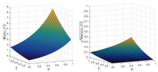
Figure 1. (Left): Surface of the expectation of the exact solution (50), $\mathbb{E}\left[u(x_i,t^n)\right]$, computed according to (51). (Right): Surface of the standard deviation of the exact solution (50), $\sqrt{\mathrm{Var}\left[u(x_i,t^n)\right]}$, computed according to (52) and (53). For both statistical moments the parameters considered in (50) are $a\sim {\mathrm{N}}_{[0.4,0.6]}(0.5;0.1)$, $c\sim {\mathrm{Beta}}_{[0.45,0.55]}(2;4)$ and the plotted domain corresponds to $(x_i=ih,t^n=nk)\in [0+h=0.0125,1-h=0.9875]\times [0.05,1]$ with the step-sizes $h=\mathsf{\Delta }x=0.0125$, $1\le i\le 79$, and $k=\mathsf{\Delta }t=0.05$, $1\le n\le 20$.

Numerical convergence of the expectation and the standard deviation of the approximate solution s.p. generated by means the sampling difference scheme (18) using the Monte Carlo (MC) technique shown in Algorithm 1, is illustrated in the following way. In the first study, with a fixed time T, we have chosen both the spatial and temporal step-sizes h and k, respectively, according to the stability conditions (21) and (23) and we have varied the number of realizations, K, of the r.v.’s a and c involved in the random problem (46)–(49). Then, at the temporal level N where the time T is achieved, we have computed the expectation (mean), ${\mathbb{E}}_{\mathrm{MC}}^K\left[u_i^N\right]$, and the standard deviation, $\sqrt{{\mathrm{Var}}_{\mathrm{MC}}^K\left[u_i^N\right]}$, of the K-deterministic solutions, $u_i^N$, obtained to solve the K-deterministic difference schemes (18). Table 1 collects the RMSEs (Root Mean Square Errors) computed at the time instant $T=Nk=1$ with the temporal step-size $k=0.0001$ (N = 10,000) for $M-1=79$ internal spatial points $x_i=ih$, $1\le i\le 79$ with $h=\mathsf{\Delta }x=0.0125$ in the domain $[0.0125,1]$, using the following expressions

$$\begin{array}{ccc}\hfill \mathrm{RMSE}\left[{\mathbb{E}}_{\mathrm{MC}}^K\left[u_i^N\right]\right]& =& \sqrt{\frac{1}{M-1}\sum _{i=1}^{M-1}{\left(\mathbb{E}\left[u(x_i,t^N)\right]-{\mathbb{E}}_{\mathrm{MC}}^K\left[u_i^N\right]\right)}^2},\hfill \end{array}$$

(54)

$$\begin{array}{ccc}\hfill \mathrm{RMSE}\left[\sqrt{{\mathrm{Var}}_{\mathrm{MC}}^K[u_i^N}]\right]& =& \sqrt{\frac{1}{M-1}\sum _{i=1}^{M-1}{\left(\sqrt{\mathrm{Var}\left[u(x_i,t^N)\right]}-\sqrt{{\mathrm{Var}}_{\mathrm{MC}}^K\left[u_i^N\right]}\right)}^2},\hfill \end{array}$$

(55)

where $\mathbb{E}\left[u(x_i,t^N)\right]$ and $\sqrt{\mathrm{Var}\left[u(x_i,t^N)\right]}$ are given by (51)–(53), respectively.

Table 1. Root mean square errors (RMSEs) at $T=Nk=1$ with $k=0.0001$ ($N0$ = 1000) for the numerical expectation and the numerical standard deviation computed after solving the K-deterministic difference scheme (18) for several Monte Carlo (MC) realizations $K\in$ {50, 200, 800, 3200, 12,800}. The spatial discretization have been considered on the domain $[0+h=0.0125,1-h=0.9875]$ with $x_i=ih$, $1\le i\le 79$, $h=0.0125$.

K	RMSE $\left[{\mathbb{E}}_{\mathbf{MC}}^{\mathit{K}}\left[{\mathit{u}}_{\mathit{i}}^{\mathit{N}}\right]\right]$	RMSE $\left[\sqrt{{\mathbf{Var}}_{\mathbf{MC}}^{\mathit{K}}\left[{\mathit{u}}_{\mathit{i}}^{\mathit{N}}\right]}\right]$
50	$1.45604\times$ 10${}^{-2}$	$1.32856\times$ 10${}^{-2}$
200	$1.11710\times$ 10${}^{-2}$	$1.84435\times$ 10${}^{-3}$
800	$1.08512\times$ 10${}^{-2}$	$1.06139\times$ 10${}^{-3}$
3200	$4.20138\times$ 10${}^{-3}$	$6.01374\times$ 10${}^{-3}$
12,800	$2.07183\times$ 10${}^{-4}$	$1.69504\times$ 10${}^{-3}$

The good behaviour of both approximations the expectation and the standard deviation as the K simulations increases was observed. That is, the accuracy of the approximations to both statistical moments increases when the number of MC simulations is growing. In this sense, Figure 2 reflects the improvement of the approximations considering the study of the relative errors computed by the expressions

$$\begin{array}{ccc}\hfill \mathrm{RelErr}\left[{\mathbb{E}}_{\mathrm{MC}}^K\left[u_i^N\right]\right]& =& \left|\frac{\mathbb{E}\left[u(x_i,t^N)\right]-{\mathbb{E}}_{\mathrm{MC}}^K\left[u_i^N\right]}{\mathbb{E}[u(x_i,t^N)]}\right|,\hfill \end{array}$$

(56)

$$\begin{array}{ccc}\hfill \mathrm{RelErr}\left(\sqrt{{\mathrm{Var}}_{\mathrm{MC}}^K\left[u_i^N\right]}\right)& =& \left|\frac{\sqrt{\mathrm{Var}\left[u(x_i,t^N)\right]}-\sqrt{{\mathrm{Var}}_{\mathrm{MC}}^K\left[u_i^N\right]}}{\sqrt{\mathrm{Var}\left[u(x_i,t^N)\right]}}\right|.\hfill \end{array}$$

(57)

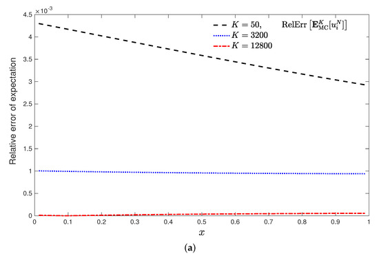
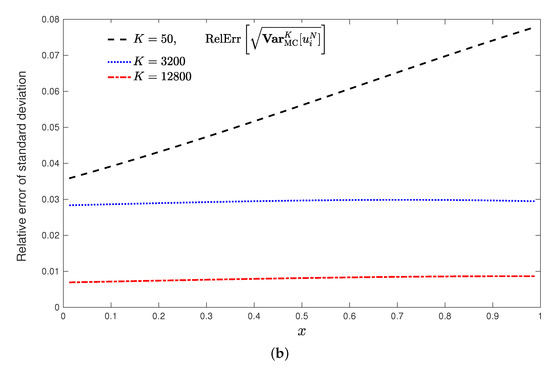
Figure 2. Plot (a): Relative errors of the approximations to the expectation (mean), ${\mathbb{E}}_{\mathrm{MC}}^K\left[u_i^N\right]$, (56). Plot (b): Relative errors of the approximations to the standard deviation, $\sqrt{{\mathrm{Var}}_{\mathrm{MC}}^K\left[u_i^N\right]}$, (57). For both graphics the fixed time horizon is $T=1=Nk$ with the temporal step-size $k=0.0001$ (N = 10,000), the spatial domain $x_i\in [0+h,1-h]$ with $x_i=ih$, $h=0.0125$, but varying the number of MC simulations $K\in$ {50, 3200, 12,800}.

Table 2 shows the second complementary study, where we have fixed the number of MC simulations K, $K=1600$, and we have refined the step-sizes h and k attending to the stability conditions (21) and (23). It is observed the decrease of the RMSEs of the expectation (54) and an apparent stabilization in the RMSEs behaviour of the standard deviation (55). Computations have been carried out by Mathematica© software version 12.0.0.0, [21] for Windows 10Pro (64-bit) AMD Ryzen Threadripper 2990WX, 3.00 GHz 32 kernels. The CPU times (in seconds) spent in the Wolfram Language kernel to compute, in both experiments, the expectation (mean) and the standard deviation are included in Table 3 and Table 4. As a result, a good strategy to study the convergence of approximations consists of choosing step-sizes h and k verifying the stability conditions and take a big enough number of realizations K such that the error does not vary significantly when one increases the number of realizations. For problems with no available solution the error is changed by the deviation between two successive numerical solutions.

Table 2. RMSEs at $T=1$ and $K=1600$ (MC simulations) for the expectation (54) and the standard deviation (55). The considered step-sizes h and k verify stability conditions (21) and (23). $T=Nk=1$, $N\in \{125,500,2000,8000\}$, the spatial domain is $[0+h,1-h]$ considering $M-1$ internal points $x_i=ih$, $1\le i\le M-1$ with $M=1/h$.

h	k	RMSE $\left[{\mathbb{E}}_{\mathbf{MC}}^{\mathit{K}}\left[{\mathit{u}}_{\mathit{i}}^{\mathit{N}}\right]\right]$	RMSE $\left[\sqrt{{\mathbf{Var}}_{\mathbf{MC}}^{\mathit{K}}\left[{\mathit{u}}_{\mathit{i}}^{\mathit{N}}\right]}\right]$
$0.1$	$0.008$	$5.29465\times {10}^{-2}$	$2.36145\times {10}^{-3}$
$0.05$	$0.002$	$3.19431\times {10}^{-3}$	$2.49070\times {10}^{-3}$
$0.025$	$0.0005$	$2.72452\times {10}^{-3}$	$2.52301\times {10}^{-3}$
$0.0125$	$0.000125$	$2.61957\times {10}^{-3}$	$2.53168\times {10}^{-3}$

Table 3. CPU time (in seconds) spent to compute the approximations to the expectation (mean), ${\mathbb{E}}_{\mathrm{MC}}^K$, and the standard deviation, $\sqrt{{\mathrm{Var}}_{\mathrm{MC}}^K}$ in Table 1, for a fixed time horizon $T=1$ and the step-sizes $h=0.0125$ and $k=0.0001$ while the number of MC simulations, K, varies.

K	CPU,s $\left[{\mathbb{E}}_{\mathbf{MC}}^{\mathit{K}}/\sqrt{{\mathbf{Var}}_{\mathbf{MC}}^{\mathit{K}}}\right]$
50	$630.516$
200	$982.375$
800	$2052.330$
3200	$6209.480$
12,800	22,600.100

Table 4. CPU time (in seconds) spent to compute the approximations to the expectation (mean), ${\mathbb{E}}_{\mathrm{MC}}^K$, and the standard deviation, $\sqrt{{\mathrm{Var}}_{\mathrm{MC}}^K}$ in Table 2, for a fixed time horizon $T=1$ and $K=1600$ MC simulations but varying the temporal step-size k and the spatial step-size h in the domain $[0+h,1-h]$.

h	k	CPU,s $\left[{\mathbb{E}}_{\mathbf{MC}}^{\mathit{K}}/\sqrt{{\mathbf{Var}}_{\mathbf{MC}}^{\mathit{K}}}\right]$
$0.1$	$0.008$	$11.4688$
$0.05$	$0.002$	$56.2344$
$0.025$	$0.0005$	$341.6410$
$0.0125$	$0.000125$	$2438.70000$

The use of MC method has allowed the obtainment of approximations to the expectation and the standard deviation of the solution s.p. $u_i^N$ of the random difference scheme (16) at time horizon $T=Nk$ for N not necessarily small. However, if we use the random numerical scheme (16) directly in this example with the step-sizes $h=0.05$ ($M=20$) and $k=0.002$ verifying the stability conditions (21) and (23), troubles appear in the early time-level $n=3$, that corresponds to time $t^n=0.006$. In this case the symbolic expressions for the random numerical solution $u_i^n$ and ${\left(u_i^n\right)}^2$, for $n=3$ are available and their correspond expectations too. However, the Mathematica© software can not compute the numerical expectation of ${\left(u_i^n\right)}^2$ for $2\le i\le 18$, $n=3$, in consequence it is not possible to compute the approximation of the standard deviation for these internal points at $t^n=0.006$ and hence at no other later time.

5. Conclusions

The main target of this paper is to solve the challenge of storage accumulation and further computational breakdown dealing with FD methods for solving random PDEM. Our approach is based on a combination of Monte Carlo method and the solution of sampled deterministic methods using explicit FD schemes. Explicitness is necessary to compute the statistical moments of the approximate solution what disregards the implicit FD methods. We here use the explicit classic difference method, but the Crank-Nicolson semi-implicit approach could be tried, making an ad hoc analysis. Numerical analysis provides sufficient conditions for positivity, stability and consistency for the proposed RMSFDS. Numerical experiments illustrate the reliability of the approach.

References

- Hundsdorfer, W.; Verwer, J.G. Numerical Solution of Time-Dependent Advection-Diffusion-Reaction Equations; Springer: New York, NY, USA, 2003. [Google Scholar]
- Smith, G.D. Numerical Solution of Partial Differential Equations: Finite Difference Methods, 3rd ed.; Clarendon Press: Oxford, UK, 1985. [Google Scholar]
- Bharucha-Reid, A.T. On the Theory of Random Equations. In Stochastic Processes in Mathematical Physics and Engineering. Proceedings of Symposia in Applied Mathematics; American Mathematical Society: Providence, PI, USA, 1964; Volume XVI, pp. 40–69. [Google Scholar]
- Bharucha-Reid, A.T. Probabilistic Methods in Applied Mathematics; Academic Press, Inc.: New York, NY, USA, 1973. [Google Scholar]
- Torquato, S. Random Heterogeneous Materials: Microstructure and Macroscopic Properties; Springer: New York, NY, USA, 2002. [Google Scholar]
- Vanmarcke, E. Random Fields: Analysis and Synthesis; World Scientific Publishing Co. Inc.: London, UK, 2010. [Google Scholar]
- Farlow, S.J. Partial Differential Equations for Scientists and Engineers; Dover: New York, NY, USA, 1993. [Google Scholar]
- Casabán, M.-C.; Company, R.; Egorova, V.; Jódar, L. Integral transform solution of random coupled parabolic partial differential models. Math. Meth. Appl. Sci. 2020, 43, 8223–8236. [Google Scholar] [CrossRef]
- Gunzburger, M.D.; Webster, C.G.; Zhang, G. Stochastic finite element methods for partial differential equations with random input data. Acta Numer. 2014, 23, 521–650. [Google Scholar] [CrossRef]
- Casabán, M.-C.; Company, R.; Jódar, L. Numerical solutions of random mean square Fisher-KPP models with advection. Math. Meth. Appl. Sci. 2020, 43, 8015–8031. [Google Scholar] [CrossRef]
- Cortés, J.-C.; Romero, J.-V.; Roselló, M.-D.; Sohaly, M.A. Solving random boundary heat model using the finite difference method under mean square convergence. Comp. Math. Meth. 2019, 1, e1026. [Google Scholar] [CrossRef]
- Sohaly, M.A. Random difference scheme for diffusion advection model. Adv. Differ. Equ. 2019, 2019, 54. [Google Scholar] [CrossRef]
- Øksendal, B. Stochastic Differential Equations. An Introduction with Applications, 5th ed.; Springer: Berlin/Heidelberg, Germany, 2003. [Google Scholar]
- Soong, T.T. Random Differential Equations in Science and Engineering; Academic Press: New York, NY, USA, 1973. [Google Scholar]
- Kroese, D.P.; Taimre, T.; Botev, Z.I. Handbook of Monte Carlo Methods; Wiley Series in Probability and Statistics; John Wiley & Sons: New York, NY, USA, 2011. [Google Scholar]
- Asmussen, S.; Glynn, P.W. Stochastic Simulation: Algorithms and Analysis; Rozovskii, B., Grimmett, G., Eds.; Springer Science & Business Media, LLC: New York, NY, USA, 2007. [Google Scholar]
- Özişik, M.N. Boundary Value Problems of Heat Conduction; Dover Publications, Inc.: New York, NY, USA, 1968. [Google Scholar]
- Polyanin, A.D.; Nazaikinskii, V.E. Handbook of Linear Partial Differential Equations for Engineers and Scientists; Taylor & Francis Group: Boca Raton, FL, USA, 2016. [Google Scholar]
- Jódar, L.; Caudillo, L.A. A low computational cost numerical method for solving mixed diffusion problems. Appl. Math. Comput. 2005, 170, 673–685. [Google Scholar] [CrossRef]
- Coatléven, J. A virtual volume method for heterogeneous and anisotropic diffusion-reaction problems on general meshes. Esaim Math. Model. Numer. Anal. 2017, 51, 797–824. [Google Scholar] [CrossRef][Green Version]
- Wolfram Research, Inc. Mathematica; Version 12.0; Mathematica Wolfram Research, Inc.: Champaign, IL, USA, 2020; Available online: https://www.wolfram.com/mathematica (accessed on 7 December 2020).
Publisher’s Note: MDPI stays neutral with regard to jurisdictional claims in published maps and institutional affiliations. |
© 2021 by the authors. Licensee MDPI, Basel, Switzerland. This article is an open access article distributed under the terms and conditions of the Creative Commons Attribution (CC BY) license (http://creativecommons.org/licenses/by/4.0/).