A New Algorithm for Computing Disjoint Orthogonal Components in the Three-Way Tucker Model

Abstract

One of the main drawbacks of the traditional methods for computing components in the three-way Tucker model is the complex structure of the final loading matrices preventing an easy interpretation of the obtained results. In this paper, we propose a heuristic algorithm for computing disjoint orthogonal components facilitating the analysis of three-way data and the interpretation of results. We observe in the computational experiments carried out that our novel algorithm ameliorates this drawback, generating final loading matrices with a simple structure and then easier to interpret. Illustrations with real data are provided to show potential applications of the algorithm.

1. Introduction

The multivariate methods offer a simplified and descriptive look at a set of multidimensional data, where individuals and variables are numerous. These data are often organized in a matrix or two-way table and, for their analysis, there is a wide theoretical background. In addition, in this context, three-way (or three-mode) tables or three-order tensors can be obtained when a new way, such as time or location, is introduced into the two-way table; see more details in [1].

Tensor decomposition emerged during the 20th century [2] and, as mentioned in [3], Tucker [4] was responsible for its use within a multivariate context in the sixties, whereas, later on, in the seventies, Harshman [5] and Carroll and Chang [6] continued the use of tensor decomposition in multivariate methods.

The analysis of three-way tables attempts to identify patterns in the space of individuals, of variables, and of times (or situations in general), searching for robust and easy-to-interpret models in order to discover how individuals and variables are related to entities in the third mode [7].

The three-way Tucker model (or Tucker3 from hereafter as Tucker) is a tensor decomposition that allows for the generalization of a principal component analysis (PCA) [8,9] to three-way tables. This multivariate method represents the original data in lower dimensional spaces, enabling pattern recognition. Furthermore, it is possible to quantify the interactions between entities in three-modes.

Similar to what occurs with a PCA, each mode of a three-way table can be represented in spaces of lower dimension than the original spaces [10]. These spaces are featured by the principal axes (components), which maximizes the total variance and they are linear combinations of the original entities [11]. Within the space of each mode, the interpretation of these axes is done in accordance with the values of their components (loadings). Therefore, interpretation can sometimes be difficult, leading to inaccurate characterization of these new axes. Thus, it is desirable that each principal component or axis has few entities that contribute to the variability of the component in a relevant manner.

There are several theoretical approaches to yield tensor decomposition that have components with some of their loadings being equal to zero. This is useful for facilitating the analysis, and the interpretation of the three-way tables, such as the sparse parallelizable tensor decomposition used in scattered components works [12]. The sparse hierarchical Tucker model focuses on factoring high order tensors [13]. In addition, the tensor truncated power searches for a sparse decomposition by choosing variables [14]. An algorithm for the sparse Tucker decomposition that sets an orthogonality condition for loading matrices and sparse conditions in the core matrix was proposed by [15].

Unlike sparse methods, disjoint methods in two-way tables search for a decomposition with a loading matrix that has a single column (latent variable) with non-zero input for each row (original variable). Furthermore, there is at least one row with a non-zero entry for each column of the loading matrix. Hence, it is possible to obtain loading matrices of simple structure that facilitate the interpretation. A method that allows for disjoint orthogonal components in a two-way table to be calculated was presented in [16]. Recently, an algorithm that is based on particle swarm optimization was proposed by [17], which consists of a disjoint PCA with constraints for the case of two-way tables. To the best of our knowledge, there are no methods for computing disjoint orthogonal components in three-way tables.

The objective of this work is to propose a heuristic algorithm that extends the existing methods of two-way tables to three-way tables. This proposal computes disjoint orthogonal components in loading matrices of a Tucker model. We introduce a procedure that suggests routes in which the proposed algorithm can be used. We call this new algorithm as DisjointTuckerALS, because this is based on the alternating least squares (ALS) method.

The remainder of the paper is organized as follows. Section 2 defines what a disjoint orthogonal matrix is and presents an optimization mathematical problem that must be solved in order to calculate disjoint orthogonal components in the Tucker model. In Section 3, we introduce the DisjointTuckerALS algorithm. Section 4 carries out the numerical applications of the present work regarding computational experiments in order to evaluate the performance of our algorithm, as well as illustrations with real data to show its potential applications. Finally, in Section 5, the conclusions of this study are provided, together with some final remarks, limitations, a wide spectrum of additional applications that are different from those presented in the illustration with real data, and ideas for future research.

2. The Tucker Model and the Disjoint Approach

In this section, we present the structure of three-way tables and define the Tucker model, as well as a disjoint approach for this model.

2.1. Three-Way Tables

A three-way table represents a data set with three-modes as individuals, variable, and situations, which is a three-dimensional array or a third-order tensor. Note that tensors have three variation modes: $\mathit{A}$-mode (with I individuals); $\mathit{B}$-mode (with J variables); and, $\mathit{C}$-mode (with K situations).

Let $\underline{\mathit{X}}$ be a three-way table of order $I\times J\times K$. The generic element $x_{ijk}$ stores the measure of individual $i\in \{1,\dots ,I\}$ in variable $j\in \{1,\dots ,J\}$ and situation $k\in \{1,\dots ,K\}$. The tensor $\underline{\mathit{X}}$ can be converted into a two-way table while using a process of matricization. In this work, we use three types of supermatrices: $\mathit{A}$-mode that yields a matrix ${\mathit{X}}_{\mathit{A}}$ of order $I\times JK$, $\mathit{B}$-mode that yields a matrix a ${\mathit{X}}_{\mathit{B}}$ of order $J\times IK$, and $\mathit{C}$-mode that yields a matrix ${\mathit{X}}_{\mathit{C}}$ of order $K\times IJ$. These supermatrices are defined as in [3], where ${\mathit{X}}_{\mathit{A}}$, ${\mathit{X}}_{\mathit{B}}$, and ${\mathit{X}}_{\mathit{C}}$ are known as frontal, horizontal, and vertical slices matrices, respectively.

2.2. The Tucker Model

Tucker is a multilinear model that approximates the three-way table $\underline{\mathit{X}}$ while using a dimensional reduction on its three-modes. The Tucker tensor decomposition of $\underline{\mathit{X}}=\left(x_{ijk}\right)$ is given by

$$x_{ijk}={\widehat{x}}_{ijk}+e_{ijk},i=1,\dots ,I,j=1,\dots ,J,k=1,\dots ,K,$$

(1)

where ${\widehat{x}}_{ijk}={\sum }_{p=1}^P{\sum }_{q=1}^Q{\sum }_{r=1}^R\left(a_{ip}{b}_{jq}{c}_{kr}{g}_{pqr}\right)$, with $a_{ip}$, $b_{jq}$, and $c_{kr}$ being the corresponding elements of the matrices $\mathit{A}=\left(a_{ip}\right)$ of order $I\times P$, $\mathit{B}=\left(b_{jq}\right)$ of order $J\times Q$, and $\mathit{C}=\left(c_{kr}\right)$ of order $K\times R$, which are called component or loading matrices. In addition, $g_{pqr}$ that is defined in (1) is the $pqr$-th element of the tensor $\underline{\mathit{G}}=\left(g_{pqr}\right)$ of order $P\times Q\times R$, which is called core and it is considered a reduced version of the tensor $\underline{\mathit{X}}$. Integers $P<I$, $Q<J$, and $R<K$ represent the number of components required on each mode, respectively. Thus, for instance, the matrix $\mathit{A}$ contains P columns that represent the new referential system of the individuals. Note that $\underline{\mathit{E}}=\left(e_{ijk}\right)$ of order $I\times J\times K$ is a tensor of model errors.

The Tucker model can be represented by matrix equations that are based on all modes [3], which are stated as

$${\mathit{X}}_{\mathit{A}}=\mathit{A}{\mathit{G}}_{\mathit{A}}{\left(\mathit{C}\otimes \mathit{B}\right)}^{\top }+{\mathit{E}}_{\mathit{A}},$$

(2)

$${\mathit{X}}_{\mathit{B}}=\mathit{B}{\mathit{G}}_{\mathit{B}}{\left(\mathit{C}\otimes \mathit{A}\right)}^{\top }+{\mathit{E}}_{\mathit{B}},$$

(3)

$${\mathit{X}}_{\mathit{C}}=\mathit{C}{\mathit{G}}_{\mathit{C}}{\left(\mathit{B}\otimes \mathit{A}\right)}^{\top }+{\mathit{E}}_{\mathit{C}},$$

(4)

where ⊗ is the Kronecker product. Furthermore, ${\mathit{G}}_{\mathit{A}}$ of order $P\times QR$, ${\mathit{G}}_{\mathit{B}}$ of order $Q\times PR$, and ${\mathit{G}}_{\mathit{C}}$ of order $R\times PQ$, defined in (2), (3), and (4), are the frontal, horizontal, and vertical slices matrices from the core $\underline{\mathit{G}}$, respectively. Observe that ${\mathit{E}}_{\mathit{A}}$, ${\mathit{E}}_{\mathit{B}}$ and ${\mathit{E}}_{\mathit{C}}$ are the corresponding error matrices.

An algorithm that is based on the ALS method and singular value decomposition (SVD) is used in order to compute the orthogonal components in the Tucker model, called the TuckerALS algorithm [10]. Note that the ALS method partitions the way of computing the three loading matrices by fixing two of them and identifying the third matrix. This is done iteratively until the matrices do not differ significantly (for example, $\left|\right|{\mathit{A}}_{\ell }-{\mathit{A}}_{\ell -1}\left|\right|<{10}^{-5}$; $\left|\right|{\mathit{B}}_{\ell }-{\mathit{B}}_{\ell -1}\left|\right|<{10}^{-5}$; $\left|\right|{\mathit{C}}_{\ell }-{\mathit{C}}_{\ell -1}\left|\right|<{10}^{-5}$), or if a maximum number of iterations (for example, 100) is attained, which are called TuckerALS stopping criteria.

The goodness-of-fit tells us how good an approximation between the original tensor and the solution that was obtained by the algorithm is. This goodness-of-fit is computed by the expression defined as

$$\mathtt{Fit}=\frac{{\sum }_{i=1}^I{\sum }_{j=1}^J{\sum }_{k=1}^K{\widehat{x}}_{ijk}^2}{{\sum }_{i=1}^I{\sum }_{j=1}^J{\sum }_{r=1}^K{x}_{ijk}^2}\times 100\%.$$

(5)

Algorithm 1 summarizes the TuckerALS method. The loading matrices $\mathit{A}$, $\mathit{B}$, $\mathit{C}$, and the supermatrix ${\mathit{G}}_{\mathit{A}}$ are the output of the TuckerALS algorithm. The DisjointTuckerALS algorithm that we propose in this paper uses an adapted version of Algorithm 1. The notation $\mathit{B}\leftarrow \mathrm{svd}({\mathit{X}}_{\mathit{B}},Q)$ means that $\mathit{B}$ is a matrix whose columns are the first Q left singular vectors of ${\mathit{X}}_{\mathit{B}}$.

Algorithm 1: TuckerALS

2.3. Disjoint Approach for the Tucker Model

Let $\mathit{X}=\left(x_{ij}\right)$ be a matrix of order $I\times J$. Afterwards, we say that $\mathit{X}$ is disjoint if and only if:

• For all $i\exists !j$, such that $x_{ij}\ne 0$.
• For all $j\exists i$, such that $x_{ij}\ne 0$.

If $\mathit{X}$ also satisfies ${\mathit{X}}^{\top }\mathit{X}={\mathit{I}}_J$, where ${\mathit{I}}_J$ is the identity matrix of order $J\times J$, we say that $\mathit{X}$ is a disjoint orthogonal matrix. The following is an example of a disjoint orthogonal matrix:

$$\mathit{X}=\left(\begin{array}{ccc}\frac{1}{\sqrt{2}}& 0& 0\\ \frac{-1}{\sqrt{2}}& 0& 0\\ 0& 1& 0\\ 0& 0& \frac{-1}{\sqrt{3}}\\ 0& 0& \frac{1}{\sqrt{3}}\\ 0& 0& \frac{-1}{\sqrt{3}}\end{array}\right).$$

The optimization mathematical problem to be solved with the DisjointTuckerALS algorithm, when the three loading matrices $\mathit{A}$, $\mathit{B}$, and $\mathit{C}$ are required to be disjoint orthogonal, is stated as

$$\begin{array}{c}\hfill \underset{\begin{array}{c}\mathit{A},\mathit{B},\mathit{C},{\mathit{G}}_{\mathit{A}}\end{array}}{min}{\parallel {\mathit{X}}_{\mathit{A}}-\underset{{\widehat{\mathit{X}}}_{\mathit{A}}}{\underbrace{\mathit{A}{\mathit{G}}_{\mathit{A}}{(\mathit{C}\otimes \mathit{B})}^{\top }}}\parallel }^2\end{array}$$

(6)

Subject to:

$$\begin{array}{ccc}\hfill {\mathit{A}}^{\top }\mathit{A}& =& {\mathit{I}}_P,\hfill \end{array}$$

(7)

$$\begin{array}{ccc}\hfill {\mathit{B}}^{\top }\mathit{B}& =& {\mathit{I}}_Q,\hfill \end{array}$$

(8)

$$\begin{array}{ccc}\hfill {\mathit{C}}^{\top }\mathit{C}& =& {\mathit{I}}_R,\hfill \end{array}$$

(9)

where $\parallel ·\parallel$ is the Frobenius norm, and ${\mathit{I}}_P,{\mathit{I}}_Q,{\mathit{I}}_R$ are identity matrices of order $P\times P$, $Q\times Q$, and $R\times R$, respectively. Note that the number of decision variables of this model is $IP$ + $JQ$ + $KR$ + $PQR$. The constraints that are given in (7)–(9) are needed in order for columns of each loading matrix to form an orthonormal set. In the previous mathematical problem, the objective function that is defined in (6) is minimized, but, in practice, the fit is calculated according to (5). In order to obtain a simple structure in a loading matrix for three-way tables, there are some known techniques called: scaling, rotation, and sparse. We propose a disjoint technique by the design and implementation of the DisjointTuckerALS algorithm. This requires a reduction of the three-modes and can be obtained up to three disjoint orthogonal loading matrices. Several methods for obtaining disjoint orthogonal components for two-way tables have been derived; see [16,18,19]. If $\mathit{A},\mathit{B},\mathit{C}$ are disjoint matrices, the mathematical model defined in (6) can be solved while using the TuckerALS method stated in Algorithm 1 and then the orthogonal components may be obtained for the Tucker model.

2.4. Illustrative Example

We show the benefit of using the DisjointTuckerALS algorithm through a computational experiment for a three-way table that was taken from [7] and adapted by [20]. This small data set is provided in Table 1, Table 2, Table 3 and Table 4, which show three-way tables with $I=6$ individuals, $J=4$ variables, and $K=4$ situations, where the behavioral levels are measured.

Table 1. Matrix of situation 1: “applying for an examen” for behavioral level data.

	Emotional	Sensitive	Caring	Thorough
Anne	0.0	0.0	4.0	4.0
Bert	0.0	0.0	2.0	2.0
Claus	0.0	0.0	2.0	2.0
Dolly	0.0	0.0	4.0	4.0
Edna	0.0	0.0	2.5	2.5
Frances	0.0	0.0	4.0	4.0

Table 2. Matrix of situation 2: “giving a speech” for behavioral level data.

	Emotional	Sensitive	Caring	Thorough
Anne	0.6	0.6	2.4	2.4
Bert	0.2	0.2	1.8	1.8
Claus	0.2	0.2	1.8	1.8
Dolly	0.6	0.6	2.4	2.4
Edna	0.4	0.4	2.1	2.1
Frances	0.6	0.6	2.4	2.4

Table 3. Matrix of situation 3: “family picnic” for behavioral level data.

	Emotional	Sensitive	Caring	Thorough
Anne	4.0	4.0	0.0	0.0
Bert	1.0	1.0	1.0	1.0
Claus	1.0	1.0	1.0	1.0
Dolly	4.0	4.0	0.0	0.0
Edna	2.0	2.0	0.5	0.5
Frances	4.0	4.0	0.0	0.0

Table 4. Matrix of situation 4: “meeting a new date” for behavioral level data.

	Emotional	Sensitive	Caring	Thorough
Anne	4.6	4.6	0.9	0.9
Bert	1.2	1.2	1.8	1.8
Claus	1.2	1.2	1.8	1.8
Dolly	4.6	4.6	0.9	0.9
Edna	2.4	2.4	1.4	1.4
Frances	4.6	4.6	0.9	0.9

The four matrices of order $6\times 4$ that are presented in Table 1, Table 2, Table 3 and Table 4 correspond to the different scenarios or situations in which the levels of behavior are evaluated. Components are chosen and the TuckerALS algorithm is executed to obtain orthogonal components, with a model fit of $99.84\%$, as in [7], and $P=Q=R=2$. When the DisjointTuckerALS algorithm is executed, the model fit is $98.10\%$.

Loading matrices $\mathit{A}$, $\mathit{B}$, and $\mathit{C}$ that were obtained with both the TuckerALS and DisjointTuckerALS algorithms are reported in Table 5, Table 6, Table 7, Table 8, Table 9 and Table 10. Disjoint orthogonal components were calculated for the loading matrices $\mathit{A}$, $\mathit{B}$, $\mathit{C}$, and reported in Table 6, Table 8, and Table 10, respectively. The first component of the loading matrix $\mathit{A}$ represents femininity and the second component masculinity; see Table 5 and Table 6. These tables allow us to affirm that the DisjointTuckerALS algorithm can identify the disjoint structure that lies in the individuals. For the loading matrix $\mathit{B}$, the first component represents the emotional state and the second component is awareness; see Table 7 and Table 8. From these tables, note that the DisjointTuckerALS algorithm is able to identify the disjoint structure in the variables. For the loading matrix $\mathit{C}$, the algorithm is able to group the four situations into two clusters; see Table 9 and Table 10. From Table 10, note that the first component is related to social situations and the second component to performance situations.

Table 5. Loading matrix $\mathit{A}$ with the TuckerALS algorithm for behavioral level data.

	Femininity	Masculinity
Anne	−0.518560994	0.2282689980
Bert	−0.2167812130	−0.619921659
Claus	−0.2167812130	−0.619921659
Dolly	−0.518560994	0.2282689980
Edna	−0.315111562	−0.2739964750
Frances	−0.518560994	0.2282689980

Table 6. Loading matrix $\mathit{A}$ with the DisjointTuckerALS algorithm for behavioral level data.

	Femininity	Masculinity
Anne	−0.545737149	0
Bert	0	−0.707106781
Claus	0	−0.707106781
Dolly	−0.545737149	0
Edna	−0.326363131	0
Frances	−0.545737149	0

Table 7. Loading matrix $\mathit{B}$ with the TuckerALS algorithm for behavioral level data.

	Emotionality	Conscientiousness
Emotional	−0.588715219	−0.3916814920
Sensitive	−0.588715219	−0.3916814920
Caring	−0.3916814920	0.588715219
Thorough	−0.3916814920	0.588715219

Table 8. Loading matrix $\mathit{B}$ with the DisjointTuckerALS algorithm for behavioral level data.

	Emotionality	Conscientiousness
Emotional	−0.707106781	0
Sensitive	−0.707106781	0
Caring	0	−0.707106781
Thorough	0	−0.707106781

Table 9. Loading matrix $\mathit{C}$ with the TuckerALS algorithm for behavioral level data.

	Social Situations	Performance Situations
Applying for an examen	−0.3331986930	0.770591276
Giving a speech	−0.3104255140	0.435143574
Family picnic	−0.538191124	−0.3872072680
Meeting a new date	−0.709200215	−0.2586690690

Table 10. Loading matrix $\mathit{C}$ with the DisjointTuckerALS algorithm for behavioral level data.

	Social Situations	Performance Situations
Applying for an examen	0	−0.827376571
Giving a speech	0	−0.561647585
Family picnic	−0.633810357	0
Meeting a new date	−0.773488482	0

Table 11 and Table 12 show the core $\underline{\mathit{G}}$ that was obtained with both of the algorithms. When observing both cores, it can be interpreted that women in social situations are mainly emotional and less aware. Conversely, men in the same situations are less emotional and more aware. In addition, in performance situations, women are mostly aware, while men are more aware than emotional in the same situations. The TuckerALS and DisjointTuckerALS algorithms yield different $\underline{\mathit{G}}$ cores, but they are interpreted in the same manner.

Table 11. Core $\underline{\mathit{G}}$ with the TuckerALS algorithm for behavioral level data.

	Social Situations		Performance Situations
	Emotionality	Conscientiousness	Emotionality	Conscientiousness
Femininity	−17.09837769	−0.489491858	0.50606476	−12.25957342
Masculinity	−0.623702797	4.106153763	0.54320104	0.72835096

Table 12. Core $\underline{\mathit{G}}$ with the DisjointTuckerALS algorithm for behavioral level data.

	Social Situations		Performance Situations
	Emotionality	Conscientiousness	Emotionality	Conscientiousness
Femininity	−15.55006689	−2.25788715	−0.883942787	−12.28278827
Masculinity	−3.12399307	−4.052179249	−0.224659034	−5.33143759

When a three-way table is analyzed while using the Tucker model, it is important to point out that the loading matrices $\mathit{A},\mathit{B}$ and $\mathit{C}$ are not always easily interpreted [7]. In many situations, these matrices need to be rotated (where any rotation is compensated in core $\underline{\mathit{G}}$) in order to identify a simple structure that allows for interpretation. However, rotating the matrices does not guarantee that a simple structure is achieved. Therefore, the use of a sparse technique would be an alternative option. Nevertheless, it is worth mentioning that we have a loss of fit when using a sparse technique, which does not happen with rotations.

It is possible to rotate only the matrix $\mathit{B}$ or, alternatively, the matrices $\mathit{B}$ and $\mathit{C}$ can be simultaneously rotated in order to obtain a simple structure, thus improving the interpretation,. However, in some cases, the data analyst can opt to rotate the three loading matrices at the same time. Similarly, in the DisjointTuckerALS algorithm, disjoint orthogonal components can be chosen in a unique matrix, for example $\mathit{B}$; in two matrices, for example $\mathit{B}$ and $\mathit{C}$; or even in the three loading matrices.

The DisjointTuckerALS algorithm was executed with the same three-way table considering all possible combinations of disjoint orthogonal components in the loading matrices $\mathit{A}$, $\mathit{B}$, and $\mathit{C}$. Table 13 reports the results of comparing different settings. From Table 13 and using the expression defined in (5), note that we lose fit when disjoint orthogonal components are required in the three loading matrices. It is important to consider that there is a loss of fit when using the disjoint technique, although interpretable loading matrices are achieved. Note that there is a tradeoff between interpretation and speed, because the DisjointTuckerALS algorithm takes longer than the TuckerALS algorithm. For details regarding the computational time (runtime) of the algorithms that are presented in Table 13, see Section 4.1.

Table 13. Comparison of fit and runtime for behavioral level data.

Disjoint Orthogonal Components	Fit (in %)	Runtime (in min)
None (TuckerALS)	99.84	0.0038
$\mathit{A}$ (DisjointTuckerALS)	99.25	0.0831
$\mathit{B}$ (DisjointTuckerALS)	99.84	0.0797
$\mathit{C}$ (DisjointTuckerALS)	98.67	0.0672
$\mathit{A}$, $\mathit{B}$ (DisjointTuckerALS)	99.25	0.0989
$\mathit{A}$, $\mathit{C}$ (DisjointTuckerALS)	98.10	0.0866
$\mathit{B}$, $\mathit{C}$ (DisjointTuckerALS)	98.67	0.0913
$\mathit{A}$, $\mathit{B}$, $\mathit{C}$ (DisjointTuckerALS)	98.10	0.1012

2.5. The DisjointPCA Algorithm

The optimization mathematical model allowing for a disjoint orthogonal loading matrix $\mathit{B}$ in a two-way table $\mathit{X}$ to be obtained is stated as

$$\begin{array}{c}\hfill \underset{\begin{array}{c}\mathit{A},\mathit{B}\end{array}}{min}{\parallel \mathit{X}-\underset{\widehat{\mathit{X}}}{\underbrace{\mathit{A}{\mathit{B}}^{\top }}}\parallel }^2\end{array}$$

(10)

subject to ${\mathit{B}}^{\top }\mathit{B}={\mathit{I}}_Q$, with $\mathit{B}$ being a disjoint matrix, where $\mathit{X}$ is the data matrix of order $I\times J$, with I individuals and J variables, $\mathit{A}$ is the scoring matrix of order $I\times Q$, and $\mathit{B}$ is the loading matrix of order $J\times Q$. Note that $Q<J$ is the number that is required for the components in the variable mode. Here, we use a greedy algorithm, known as the DisjointPCA algorithm proposed by [16], in order to find a solution to the minimization problem defined in (10). The DisjointPCA algorithm plays a fundamental role for the operation of the DisjointTuckerALS algorithm.

The notation $\mathit{B}\leftarrow \mathrm{vs}(\mathit{X},Q,\mathtt{Tol})$ means that the DisjointPCA algorithm with a tolerance Tol is applied to the data matrix $\mathit{X}$, and then the disjoint orthogonal loading matrix $\mathit{B}$, with Q components, is obtained as a result. Recall that the DisjointPCA algorithm was proposed by Vichi and Saporta [16] reason why we use the acronym “vs" in the above notation. Note that Tol is a tolerance parameter that represents the maximum distance allowed in the model fit for two consecutive iterations of the DisjointPCA algorithm. The above notation is used in order to explain how the DisjointTuckerALS algorithm works; see [16,21] for more details on the DisjointPCA algorithm.

3. The DisjointTuckerALS Algorithm

In this section, we derive the DisjointTuckerALS algorithm in order to compute from one to three disjoint orthogonal loading matrices for the Tucker model. Next, we explain how the DisjointTuckerALS algorithm works.

3.1. The Stages of the Algorithm

The DisjointTuckerALS algorithm has three stages and its input parameters are:

• $\underline{\mathit{X}}$: Three-way table of data;
• $P,Q,R$: Number of components in $\mathit{A}$-mode, $\mathit{B}$-mode, $\mathit{C}$-mode, respectively;
• ALSMaxIter: Maximum number of iterations of the ALS algorithm; and
• Tol: Maximum distance allowed in the fit of the model for two consecutive iterations of the DisjointPCA algorithm.

Stage 1 

[Initial computation of loading matrices with an adapted TuckerALS algorithm]

In this first stage, an initial calculation of the loading matrices is made. To do this, an adapted TuckerALS algorithm is executed, as defined in Algorithm 2. The output in Algorithm 2 are the matrices ${\mathit{Y}}_{\mathit{A}}$, ${\mathit{Y}}_{\mathit{B}}$, and ${\mathit{Y}}_{\mathit{C}}$ of order $I\times QR$, $J\times PR$, and $K\times PQ$, respectively.

Algorithm 2: Adapted TuckerALS

Stage 2 

[Computation of disjoint orthogonal loading matrices with the DisjointPCA algorithm]

This second stage is where the disjoint orthogonal loading matrices are computed. In order to obtain P, Q, and R disjoint orthogonal components in the loading matrices $\mathit{A}$, $\mathit{B}$, and $\mathit{C}$, the DisjointPCA algorithm is applied to the matrices ${\mathit{Y}}_{\mathit{A}}^{\top }$, ${\mathit{Y}}_{\mathit{B}}^{\top }$ and ${\mathit{Y}}_{\mathit{C}}^{\top }$, respectively. If $\mathit{A}$ is required to be disjoint orthogonal, then we have that: $\mathit{A}\leftarrow \mathrm{vs}({\mathit{Y}}_{\mathit{A}}^{\top },P,\mathtt{Tol})$. If $\mathit{B}$ is required to be disjoint orthogonal, then we have that: $\mathit{B}\leftarrow \mathrm{vs}({\mathit{Y}}_{\mathit{B}}^{\top },Q,\mathtt{Tol})$. If $\mathit{C}$ is required to be disjoint orthogonal, then we have that: $\mathit{C}\leftarrow \mathrm{vs}({\mathit{Y}}_{\mathit{C}}^{\top },R,\mathtt{Tol})$.

Stage 3 

[Computation of non-disjoint orthogonal loading matrices and of the core]

This final stage is where the non-disjoint orthogonal loading matrices are computed. For instance, if it is required that only the matrix $\mathit{B}$ has disjoint orthogonal components (see Figure 1), then an ALS algorithm must be applied in order to compute loading matrices $\mathit{A}$ and $\mathit{C}$ (with the $\mathit{B}$ matrix being fixed). The same occurs in the TuckerALS algorithm, initializing $\mathit{A}$ or $\mathit{C}$. In addition, if it is required that the matrices $\mathit{B}$ and $\mathit{C}$ have disjoint orthogonal components (see Figure 2), then the loading matrix $\mathit{A}$ is calculated while using the following two steps (the matrices $\mathit{B}$ and $\mathit{C}$ are fixed), as in the TuckerALS algorithm: (1) ${\mathit{Y}}_{\mathit{A}}\leftarrow {\mathit{X}}_{\mathit{A}}\left(\mathit{C}\otimes \mathit{B}\right)$; and (2) $\mathit{A}\leftarrow \mathrm{svd}\left({\mathit{Y}}_{\mathit{A}},P\right)$. If $\mathit{A}$, $\mathit{B}$ and $\mathit{C}$ are required to be disjoint orthogonal (see Figure 3), then no calculation is necessary in the loading matrices. Therefore, the DisjointTuckerALS algorithm must compute the core while using two steps. Thus, by using the frontal slices equation from $\underline{\mathit{G}}$, we have that: (1) ${\mathit{Y}}_{\mathit{A}}\leftarrow {\mathit{X}}_{\mathit{A}}\left(\mathit{C}\otimes \mathit{B}\right)$; and (2) ${\mathit{G}}_{\mathit{A}}\leftarrow {\mathit{A}}^{\top }{\mathit{Y}}_{\mathit{A}}$. The DisjointTuckerALS algorithm finishes by providing the matrices $\mathit{A}$, $\mathit{B}$ and $\mathit{C}$, the core $\underline{\mathit{G}}$, and the fit of the model.

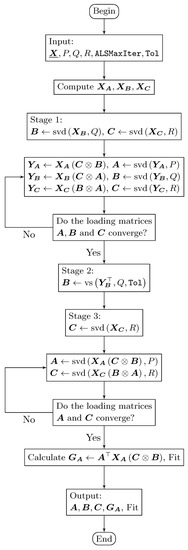
Figure 1. Flowchart of the DisjointTuckerALS algorithm that computes a single disjoint orthogonal matrix (in this case, the matrix $\mathit{B}$).

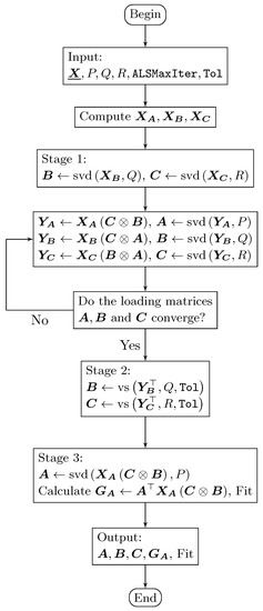
Figure 2. Flowchart of the DisjointTuckerALS algorithm that computes two disjoint orthogonal matrices (in this case the matrices $\mathit{B}$ and $\mathit{C}$).

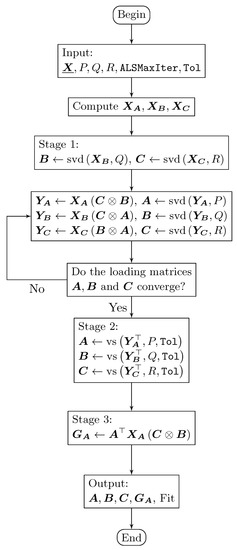
Figure 3. Flowchart of the DisjointTuckerALS algorithm that computes three disjoint orthogonal matrices: $\mathit{A}$, $\mathit{B}$, and $\mathit{C}$.

3.2. Using the DisjointTuckerALS Algorithm

We summarize our proposal in Algorithm 3 in order to explain the use of the DisjointTuckerALS algorithm when performing a component analysis for three-way tables with the Tucker model.

Computing the disjoint orthogonal components in Step 7 simultaneously in the three loading matrices is up to the analyst. However, it is not recommendable, due to the significant loss of fit that we have observed in the different computational experiments that were carried out. When more disjoint orthogonal loading matrices are computed, there is less fit in the model and more processing time is required. More than one technique can be used by combining Step 5, Step 6, and Step 7. Subsequently, the results can be compared in Step 8; see Figure 4.

Algorithm 3: Procedure for using DisjointTuckerALS

Step 1. Collect the data in a three-way table $\underline{\mathit{X}}$ of order $I\times J\times K$, where I is the number of individuals, J is the number of variables, and K is the number of situations. Step 2. Preprocess $\underline{\mathit{X}}$ according to the analyst’s criterion. Step 3. Determine the number of components P, Q and R on each mode, $\mathit{A}$-mode, $\mathit{B}$-mode and $\mathit{C}$-mode, respectively. Step 4. Perform a usual PCA with the tensor $\underline{\mathit{X}}$, that is, compute the loading matrices for example with the TuckerALS algorithm. If the loading matrices $\mathit{A}$, $\mathit{B}$ and $\mathit{C}$ have a simple structure (easy to interpret), go to Step 8. Step 5. Apply either scaling or rotation techniques to keep the fit. If the loading matrices have a simple structure, go to Step 8. Step 6. Use a sparse technique. If the loading matrices are simple, go to Step 8. Step 7. Employ a disjoint technique by computing disjoint orthogonal components using the DisjointTuckerALS algorithm, and continue to Step 8. Step 8. Report the results and obtain conclusions.

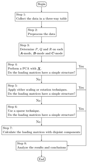
Figure 4. Flowchart for using the DisjointTuckerALS algorithm.

4. Numerical Results

In this section, we carry out computational experiments in order to evaluate the performance of our algorithm. The first experiment corresponds to data that are simulated to generate a three-way table with a disjoint structure according to the Tucker model. The second one is an experiment using real data that correspond to a three-way table taken from [22]. In this section, we also provide details of some computational aspects, such as runtimes of the algorithm, characteristics of the hardware, and software used, among others.

4.1. Computational Aspects

We must mention that the DisjointTuckerALS algorithm requires more computational time (runtime) than the TuckerALS algorithm. This is explained, because, as the number of loading matrices calculated as disjoint increases, the time that is required for their calculation also increases, consuming more computational resources of memory and processor.

The computational experiments were carried out on a computer with the following hardware characteristics: (i) OS: Windows 10 for 64 bits; (ii) RAM: 8 Gigabytes; and (iii) processor: Intel Core i7-4510U 2-2.60 GHZ. Regarding the software, the following tools and programming languages were used: (i) development tool—IDE—: Microsoft Visual Studio Express; (ii) programming language: C#.NET; and, (iii) statistical software: R.

The DisjointPCA, TuckerALS, and DisjointTuckerALS algorithms that are presented in this paper to perform all of the numerical applications were implemented in C#.NET as the programming language mainly for the graphical user interface (GUI) of data entry, control of calculations, and delivery of results. Data entry and presentation of results were carried out with Excel sheets. Communication between C#.NET and Excel was established through a connector known as COM+. Some parts of the codes developed were implemented while using the R programming language for random number generation and SVD. Communication between C#.NET and R was stated with R.NET as a connector, which can be installed in Visual Studio with a package named NuGet, whereas SVD was performed with an R package named irlba. This package quickly calculates the partial SVD, that is, those SVD which use the first singular values, but we must specify the number of singular values to be calculated. Therefore, the irlba package does not use nor compute the other singular values, accelerating the calculations for big matrices, such as frontal, horizontal, and vertical slices matrices of a three-way table.

4.2. Generator of Disjoint Structure Tensors

We design and implement a simulation algorithm to randomly build a three-way table with a disjoint latent structure in its three-modes. Subsequently, the DisjointTuckerALS algorithm should be able to detect that structure, since it uses a Tucker model with disjoint orthogonal components.

Let $\underline{\mathit{X}}$ be a three-way table with I individuals, J variables, and K times or locations. Assume that: (i) the first mode, which is related to the loading matrix $\mathit{A}$, has P latent individuals ($P<I$); (ii) the second mode, which is related to the loading matrix $\mathit{B}$, has Q latent variables ($Q<J$); and, (iii) the third mode, which is related to the loading matrix $\mathit{C}$, has R latent locations ($R<K$). Suppose that ${sx}_1,\dots ,{sx}_I$ are the I original individuals. In addition, ${sy}_1,\dots ,{sy}_P$ are the P latent individuals. We consider the linear combination that is given by

$$s{y}_p=a_{1,p}s{x}_1+\cdots +a_{I,p}s{x}_I,p=1,\dots ,P.$$

(11)

If it is required that the m original consecutive individuals, $s{x}_n,s{x}_{n+1},\cdots ,s{x}_{n+\left(m-1\right)}$, are represented by the latent individual $s{y}_p$, then the scalars $a_{n,p},a_{n+1,p},\cdots ,a_{n+\left(m-1\right),p}$ are defined as independent random variables with discrete uniform distribution, whose support is the closed set of integer numbers from 70 to 100. The other scalars in the same linear combination are defined as independent random variables with discrete uniform distribution, whose support is the closed set of integer numbers from one to 30. This procedure must be performed for each p from 1 to P, since each original individual must have a strong presence in a unique latent individual. The Gram–Schmidt orthonormalization process is applied to the matrix of order $I\times P$, which has the scalars from all the linear combinations. Hence, a disjoint dimensional reduction of the loading matrix $\mathit{A}$ is achieved.

Similarly with the loading matrix $\mathit{B}$, consider that ${vx}_1,\dots ,{vx}_J$ are the J original variables. In addition, ${vy}_1,\dots ,{vy}_Q$ are the Q latent variables. We consider the linear combination that is stated as

$$v{y}_q=b_{1,q}v{x}_1+\cdots +b_{J,q}v{x}_J,q=1,\dots ,Q.$$

(12)

If it is required that the m consecutive original variables $v{x}_n,v{x}_{n+1},\dots ,v{x}_{n+\left(m-1\right)}$ are represented by the latent variable ${vy}_q$, then the scalars $b_{n,q},b_{n+1,q},\dots ,b_{n+\left(m-1\right),q}$ are defined as independent random variables with discrete uniform distribution, similarly as for the matrix $\mathit{A}$. In the same manner as before, this procedure must be performed for each q from 1 to Q and the Gram–Schmidt orthonormalization process is again applied, as in the case of $\mathit{A}$, and then a disjoint dimensional reduction of $\mathit{B}$ is achieved.

Analogously with $\mathit{C}$, let ${tx}_1,\dots ,{tx}_K$ be the K times or original locations and ${ty}_1,\dots ,{ty}_R$ be the R latent times or latent locations. We consider the linear combination that is expressed by

$$t{y}_r=c_{1,r}t{x}_1+\dots +c_{K,r}t{x}_K,r=1,\dots ,R.$$

(13)

If it is required that the m consecutive original locations $t{x}_n,t{x}_{n+1},\dots ,t{x}_{n+(m-1)}$ are represented by the latent location $t{y}_r$, then the scalars $c_{n,r},c_{n+1,r},\dots ,c_{n+\left(m-1\right),r}$ are defined as with $\mathit{A}$ and $\mathit{B}$, and the procedure is applied for each r from 1 to R. Once again, the Gram–Schmidt orthonormalization process is applied to the matrix of order $K\times R$ that has the scalars from all of the linear combinations. Thus, a disjoint dimensional reduction of the loading matrix $\mathit{C}$ is achieved.

The Core $\underline{\mathit{G}}$ must be of order $P\times Q\times R$. With no loss of generality, suppose that the inputs of that three-way table are independent random variables with continuous uniform distribution in the interval $\left[-50.50\right]$. In order to complete the creation of $\underline{\mathit{X}}$, the matrix equation is defined as

$${\mathit{X}}_{\mathit{A}}=\mathit{A}{\mathit{G}}_{\mathit{A}}{\left(\mathit{C}\otimes \mathit{B}\right)}^{\top }.$$

(14)

The matrix ${\mathit{X}}_{\mathit{A}}$ of order $I\times JK$ stated in (14) has the frontal slices of $\underline{\mathit{X}}$, whereas the matrix ${\mathit{G}}_{\mathit{A}}$ of order $P\times QR$ has the frontal slices of $\underline{\mathit{G}}$. Equations (11)–(13) are used in order to build the random loading matrices. The algorithm that builds the three-way random table $\underline{\mathit{X}}$ of order $I\times J\times K$ must implement an application $\mathit{\phi }$ that is expressed as

$$\begin{array}{ccc}\hfill \mathit{\phi }:{\mathbb{N}}^6\times {\mathbb{N}}^P\times {\mathbb{N}}^Q\times {\mathbb{N}}^R& \to & {\mathrm{T}}_{I\times J\times K}\hfill \\ \hfill \left(\left\{I,J,K,P,Q,R\right\},{\left\{{\alpha }_p\right\}}_{p=1}^P,{\left\{{\beta }_q\right\}}_{q=1}^Q,{\left\{{\gamma }_r\right\}}_{r=1}^R\right)& \mapsto & \mathit{\phi }\left(\left\{I,J,K,P,Q,R\right\},{\left\{{\alpha }_p\right\}}_{p=1}^P,{\left\{{\beta }_q\right\}}_{q=1}^Q,{\left\{{\gamma }_r\right\}}_{r=1}^R\right),\hfill \end{array}$$

(15)

which is subject to $P<I$, $Q<J$ and $R<K$, where ${\mathrm{T}}_{I\times J\times K}$ is the set of all three-way tables with entries in the real numbers. Additionally, it must satisfy that

$$I=\sum _{p=1}^P{\alpha }_p,J=\sum _{q=1}^Q{\beta }_q,K=\sum _{r=1}^R{\gamma }_r,$$

(16)

where ${\alpha }_p$ is the number of original individuals in the p-th latent individual; ${\beta }_q$ is the number of original variables in the q-th latent variable; and ${\gamma }_r$ is the number of original locations in the r-th latent location. The application $\mathit{\phi }$ that is defined in (15) must randomly provide a three-way table $\underline{\mathit{X}}$ of order $I\times J\times K$ that has a simple structure, which is expected to be detected by the DisjointTuckerALS algorithm.

4.3. Applying the DisjointTuckerALS Algorithm to Simulated Data

Next, we show how the DisjointTuckerALS algorithm works by using the application $\mathit{\phi }$ in order to generate a three-way table $\underline{\mathit{X}}$ of order $20\times 18\times 17$. According to the definition of $\mathit{\phi }$ given in (15), the values of P, Q, R are $3,4$ and 5 respectively. Furthermore, constraints stated in (16) are satisfied. The other parameter setting is given by $\mathtt{ALSMaxIter}=100$ and $\mathtt{Tol}=0.00001$. The TuckerALS and DisjointTuckerALS algorithms were executed while using the data $\mathit{\phi }(20,18,17,3,4,5$, $\{5,7,8\}$, $\{3,4,5,6\}$, $\{2,3,3,4,5\})$, obtaining a fit of $94.73\%$ and $92.79\%$, respectively; see Table 14. As expected, we have a loss of fit valued at 1.94%. However, there is a gain in interpretation, because a simple structure in the three loading matrices is obtained. Table 15 reports the loading matrix $\mathit{A}$. Note that the DisjointTuckerALS algorithm is able to identify the disjoint structure in the first mode. Observe that five original individuals are represented by the first disjoint orthogonal component. The next seven original individuals are represented by the second disjoint orthogonal component. In addition, the last eight original individuals are represented by the third disjoint orthogonal component. Table 16 shows the loading matrix $\mathit{B}$. The fact that the DisjointTuckerALS algorithm is able to identify a disjoint structure in the second mode is highlighted. The algorithm is able to recognize the way in which the latent variables group the original variables. Table 17 presents the loading matrix $\mathit{C}$ and, once again, note that the DisjointTuckerALS algorithm identifies the disjoint structure in the third mode.

Table 14. Comparison of fit and runtime for simulated data.

Algorithm	Fit (in %)	Runtime (in min)
TuckerALS	94.73	0.0717
DisjointTuckerALS	92.79	0.8735

Table 15. Loading matrix $\mathit{A}$ with the DisjointTuckerALS algorithm for simulated data.

	${\mathit{sy}}_1$	${\mathit{sy}}_2$	${\mathit{sy}}_3$
${\mathit{sx}}_{\mathbf{1}}$	0.48932151	0	0
${\mathit{sx}}_{\mathbf{2}}$	0.44138634	0	0
${\mathit{sx}}_{\mathbf{3}}$	0.38687825	0	0
${\mathit{sx}}_{\mathbf{4}}$	0.40775562	0	0
${\mathit{sx}}_{\mathbf{5}}$	0.49980310	0	0
${\mathit{sx}}_{\mathbf{6}}$	0	0.39376793	0
${\mathit{sx}}_{\mathbf{7}}$	0	0.36369995	0
${\mathit{sx}}_{\mathbf{8}}$	0	0.39165864	0
${\mathit{sx}}_{\mathbf{9}}$	0	0.37564528	0
${\mathit{sx}}_{\mathbf{10}}$	0	0.43001693	0
${\mathit{sx}}_{\mathbf{11}}$	0	0.31146907	0
${\mathit{sx}}_{\mathbf{12}}$	0	0.36910128	0
${\mathit{sx}}_{\mathbf{13}}$	0	0	−0.32559414
${\mathit{sx}}_{\mathbf{14}}$	0	0	−0.33366963
${\mathit{sx}}_{\mathbf{15}}$	0	0	−0.31117803
${\mathit{sx}}_{\mathbf{16}}$	0	0	−0.36099787
${\mathit{sx}}_{\mathbf{17}}$	0	0	−0.34156470
${\mathit{sx}}_{\mathbf{18}}$	0	0	−0.38518722
${\mathit{sx}}_{\mathbf{19}}$	0	0	−0.37839893
${\mathit{sx}}_{\mathbf{20}}$	0	0	−0.38377130

Table 16. Loading matrix $\mathit{B}$ with the DisjointTuckerALS algorithm for simulated data.

	${\mathit{vy}}_1$	${\mathit{vy}}_2$	${\mathit{vy}}_3$	${\mathit{vy}}_4$
${\mathit{vx}}_{\mathbf{1}}$	−0.63185677	0	0	0
${\mathit{vx}}_{\mathbf{2}}$	−0.53495062	0	0	0
${\mathit{vx}}_{\mathbf{3}}$	−0.56087864	0	0	0
${\mathit{vx}}_{\mathbf{4}}$	0	−0.54058450	0	0
${\mathit{vx}}_{\mathbf{5}}$	0	−0.51277877	0	0
${\mathit{vx}}_{\mathbf{6}}$	0	−0.54593785	0	0
${\mathit{vx}}_{\mathbf{7}}$	0	−0.38311642	0	0
${\mathit{vx}}_{\mathbf{8}}$	0	0	−0.43631239	0
${\mathit{vx}}_{\mathbf{9}}$	0	0	−0.46432965	0
${\mathit{vx}}_{\mathbf{10}}$	0	0	−0.45681443	0
${\mathit{vx}}_{\mathbf{11}}$	0	0	−0.45592570	0
${\mathit{vx}}_{\mathbf{12}}$	0	0	−0.42128590	0
${\mathit{vx}}_{\mathbf{13}}$	0	0	0	0.48405851
${\mathit{vx}}_{\mathbf{14}}$	0	0	0	0.47246029
${\mathit{vx}}_{\mathbf{15}}$	0	0	0	0.36140660
${\mathit{vx}}_{\mathbf{16}}$	0	0	0	0.40851941
${\mathit{vx}}_{\mathbf{17}}$	0	0	0	0.35273551
${\mathit{vx}}_{\mathbf{18}}$	0	0	0	0.34719369

Table 17. Loading matrix $\mathit{C}$ with DisjointTuckerALS algorithm for simulated data.

	${\mathit{ty}}_1$	${\mathit{ty}}_2$	${\mathit{ty}}_3$	${\mathit{ty}}_4$	${\mathit{ty}}_5$
${\mathit{tx}}_{\mathbf{1}}$	0.56826144	0	0	0	0
${\mathit{tx}}_{\mathbf{2}}$	0.82284806	0	0	0	0
${\mathit{tx}}_{\mathbf{3}}$	0	0.50066252	0	0	0
${\mathit{tx}}_{\mathbf{4}}$	0	0.57846089	0	0	0
${\mathit{tx}}_{\mathbf{5}}$	0	0.64398760	0	0	0
${\mathit{tx}}_{\mathbf{6}}$	0	0	0.62935973	0	0
${\mathit{tx}}_{\mathbf{7}}$	0	0	0.65899658	0	0
${\mathit{tx}}_{\mathbf{8}}$	0	0	0.41186143	0	0
${\mathit{tx}}_{\mathbf{9}}$	0	0	0	0.40455206	0
${\mathit{tx}}_{\mathbf{10}}$	0	0	0	0.52191470	0
${\mathit{tx}}_{\mathbf{11}}$	0	0	0	0.47595483	0
${\mathit{tx}}_{\mathbf{12}}$	0	0	0	0.58086976	0
${\mathit{tx}}_{\mathbf{13}}$	0	0	0	0	0.50933537
${\mathit{tx}}_{\mathbf{14}}$	0	0	0	0	0.44032157
${\mathit{tx}}_{\mathbf{15}}$	0	0	0	0	0.34018158
${\mathit{tx}}_{\mathbf{16}}$	0	0	0	0	0.36337834
${\mathit{tx}}_{\mathbf{17}}$	0	0	0	0	0.54674224

The DisjointTuckerALS algorithm also recognizes the manner in which the latent locations group the original locations and the three loading matrices are easily interpreted. However, when running the TuckerALS algorithm, the three loading matrices do not allow for an easy interpretation. Note that the disjoint approach can be complemented with rotations and sparse techniques for better analysis.

4.4. Applying the DisjointTuckerALS Algorithm to Real Data

Next, the DisjointTuckerALS algorithm is executed with a three-way table $\underline{\mathit{X}}$ of order $24\times 20\times 38$ with real data being taken from [22]. Note that $K=38$ Japanese university students evaluate $I=24$ Chopin’s preludes while using $J=20$ bipolar scales. The preprocessing of the data and the number of components in each mode have been chosen in the same manner, as in [22]. Table 18 reports the model fit in four different scenarios with $P=2$, $Q=3$, and $R=2$. The full data set can be downloaded from http://three-mode.leidenuniv.nl.

Table 18. Comparison of fit and runtime for Chopin’s preludes data.

Disjoint Orthogonal Components	Fit (in %)	Runtime (in min)
NONE (TuckerALS)	42.63	0.0711
$\mathit{A}$ (DisjointTuckerALS)	38.92	0.4171
$\mathit{B}$ (DisjointTuckerALS)	40.24	0.4808
$\mathit{A}$, $\mathit{B}$ (DisjointTuckerALS)	36.79	0.7136

For a comparative analysis, the loading matrix that is related to Chopin’s preludes is chosen. Table 19 reports the loading matrix $\mathit{A}$ obtained while using the TuckerALS algorithm. In [22], this matrix is not interpreted and they proceed to make rotations.

Table 19. Loading matrix $\mathit{A}$ obtained with the TuckerALS algorithm for Chopin’s preludes data.

Chopin’s Preludes	Comp1	Comp2
(1) C major Agitato	−0.033953528	0.184842162
(2) a minor Lento	−0.137757855	−0.362945929
(3) G major Vivace	0.183142589	0.335407766
(4) e minor Largo	−0.046034600	−0.290603627
(5) D major Allegro	0.204062480	0.200322397
(6) b minor Lento assai	−0.109263322	−0.337194080
(7) A major Andantino	0.322239475	−0.165253184
(8) f# minor Molto agitato	−0.131497358	0.103731974
(9) E major Largo	−0.191131130	−0.199220960
(10) c# minor Allegro molto	0.060345767	0.118857312
(11) B major Vivace	0.270309648	−0.021135215
(12) g# minor Presto	−0.174159755	0.154464730
(13) F# major Lento	0.124820434	−0.196316896
(14) eb minor Allegro	−0.200476583	0.134265782
(15) Db major Sostenuto	0.317539137	−0.189612402
(16) bb minor Presto con fuoco	−0.13411733	0.374842648
(17) Ab major Allegretto	0.039035613	−0.099661458
(18) f minor Allegro molto	−0.297127956	0.124019724
(19) Eb major Vivace	0.228844926	0.119167072
(20) c minor Largo	−0.225976898	−0.225192986
(21) Bb major Cantabile	0.144306691	−0.085136044
(22) g minor Molto agitato	−0.269583704	0.074670854
(23) F major Moderato	0.313700444	0.137709411
(24) d minor Allegro appasionato	−0.257267184	0.109970949

Table 20 provides the final loading matrix $\mathit{A}$ used for interpretation. The first component is named “fast+minor, slow+major” and the second component is named “fast+major, slow+minor”. Table 21 presents the loading matrix $\mathit{A}$ that was obtained with the DisjointTuckerALS algorithm. Note that, with the loading matrix $\mathit{A}$ of Table 21, the same conclusions are reached as with the loading matrix $\mathit{A}$ of Table 20.

Table 20. Loading matrix $\mathit{A}$ obtained by rotations for Chopin’s preludes data.

Chopin’s Preludes	Fast + Minor, Slow + Major	Fast + Major, Slow + Minor
(1) C major Agitato	0.153	0.109
(2) a minor Lento	−0.155	−0.356
(3) G major Vivace	0.103	0.368
(4) e minor Largo	−0.170	−0.240
(5) D major Allegro	0.006	0.286
(6) b minor Lento assai	−0.157	−0.318
(7) A major Andantino	−0.346	0.107
(8) f# minor Molto agitato	0.167	0.018
(9) E major Largo	−0.003	−0.276
(10) c# minor Allegro molto	0.040	0.127
(11) B major Vivace	−0.208	0.174
(12) g# minor Presto	0.232	−0.011
(13) F# major Lento	−0.227	−0.053
(14) eb minor Allegro	0.237	−0.044
(15) Db major Sostenuto	−0.360	0.086
(16) bb minor Presto con fuoco	0.358	0.174
(17) Ab major Allegretto	−0.098	−0.044
(18) f minor Allegro molto	0.299	−0.119
(19) Eb major Vivace	−0.080	0.245
(20) c minor Largo	−0.004	−0.319
(21) Bb major Cantabile	−0.163	0.040
(22) g minor Molto agitato	0.245	−0.135
(23) F major Moderato	−0.128	0.318
(24) d minor Allegro appasionato	0.261	−0.101

Table 21. Loading matrix $\mathit{A}$ obtained with the DisjointTuckerALS algorithm for Chopin’s data.

Chopin’s Preludes	Fast + Minor, Slow + Major	Fast + Major, Slow + Minor
(1) C major Agitato	0.091495243	0
(2) a minor Lento	0	−0.349499568
(3) G major Vivace	0	0.380083836
(4) e minor Largo	0	−0.216381495
(5) D major Allegro	0	0.322563112
(6) b minor Lento assai	0	−0.306829783
(7) A major Andantino	−0.391407119	0
(8) f# minor Molto agitato	0.170783607	0
(9) E major Largo	0	−0.308357327
(10) c# minor Allegro molto	0	0.130529712
(11) B major Vivace	−0.292993592	0
(12) g# minor Presto	0.231153448	0
(13) F# major Lento	−0.191308850	0
(14) eb minor Allegro	0.252789215	0
(15) Db major Sostenuto	−0.393591840	0
(16) bb minor Presto con fuoco	0.254710019	0
(17) Ab major Allegretto	−0.071449806	0
(18) f minor Allegro molto	0.352314932	0
(19) Eb major Vivace	0	0.300266062
(20) c minor Largo	0	−0.359417233
(21) Bb major Cantabile	−0.178560495	0
(22) g minor Molto agitato	0.308258927	0
(23) F major Moderato	0	0.396120182
(24) d minor Allegro appasionato	0.305864985	0

5. Conclusions, Discussion, Limitations, and Future Research

The main techniques for dimensionality reduction, pattern extraction, and classification in data obtained through tensorial analysis have been based on the Tucker model. However, a big problem of the existing techniques is the interpretability of their results. In this work, we have proposed a heuristic algorithm for computing the disjoint orthogonal components in a three-way table with the Tucker model, which facilitates the mentioned interpretability. The DisjointTuckerALS algorithm is based on a combination of the TuckerALS and DisjointPCA algorithms. The results that were obtained in the computational experiments have shown that the main benefit of the proposed algorithm is its easiness of direct interpretation in the loading matrices without using rotational methods or sparse techniques. Computational experiments have suggested that the algorithm can detect and catch disjoint structures in a three-way table according to the Tucker model. In summary, this paper reported the following findings:

(i)

A new algorithm for computing disjoint orthogonal components in a three-way table with the Tucker model was proposed.

(ii)

A measure of goodness of fit to evaluate the algorithms presented was proposed.

(iii)

A optimization mathematical model was used.

(iv)

A numerical evaluation of the proposed methodology was considered by means of Monte Carlo simulations.

(v)

By using a case study with real-world data, we have illustrated the new algorithm.

Numerical experiments of the proposed algorithm with simulated and real data sets allowed us to show its good performance and its potential applications. We obtained a new algorithm that can be a useful knowledge addition to the multivariate tool-kit of diverse practitioners, applied statisticians, and data scientists.

Some limitations of our study, which could be improved in future works are the following:

(i)

There is no guarantee that the optimal solution is attained due to the heuristic nature of the DisjointTuckerALS algorithm.

(ii)

In the absence of additional constraints to those inherent to the original problem, the space of feasible solutions contains the global optimum. However, by incorporating the constraints of the DisjointTuckerALS algorithm, the space of feasible solutions is compressed, which aims to find a solution that is as close as possible to the global optimum within this new set of feasible solutions. For this reason, the fit corresponding to the solution provided by the DisjointTuckerALS algorithm is less than the fit achieved by the TuckerALS algorithm. Nevertheless, the incorporated constraints allow us to put zeros in the positions of the variables with low contribution into a component of the loading matrix, which permits us to interpret the components more clearly.

(iii)

The proposed algorithm takes longer than the TuckerALS algorithm, so that a tradeoff between interpretation and speed exists.

In order to motivate readers and potential users, a wide spectrum of additional applications of the new algorithm with real three-way data in diverse areas is the following:

(i)

Functional magnetic resonance imaging (fMRI) has been successfully used by the neuroscientists for diagnosis of neurological and neurodevelopmental disorders. The fMRI has been analyzed by means of tensorial methods while using the Tucker model [23].

(ii)

Component analysis in three-way tables also has application in environmental sciences. For example, in [24], through the multivariate study of a sample of blue crabs, a hypothesis is tested that environmental stress weakens some organisms, since the normal immune response is not able to protect them from a bacterial infection. A Tucker model was used for this analysis.

(iii)

The data of the price indexes in search of behavior patterns using the Tucker decomposition were analyzed in [25]. The DisjointTuckerALS algorithm can be used for detecting these patterns.

(iv)

An application in economy on the specialization indexes of the electronic industries of 23 European countries of the Organisation for Economic Co-operation and Development (OECD) based on three-way tables is presented in [1]; see also http://three-mode.leidenuniv.nl. Applications in stock markets and breakpoint analysis for the COVID-19 pandemic can be also considered [26].

(v)

On the website "The Three-Mode Company” (see http://three-mode.leidenuniv.nl), data sets corresponding to three-way tables, including engineering, management, and medicine, are related to (a) aerosol particles in Austria; (b) diseased blue crabs in the US; (c) chromatography; (d) coping Dutch primary school children; (e) Dutch hospitals as organizations; (f) girls’ growth curves between five and 15 years old; (g) happiness, siblings, and schooling; (h) multiple personalities; (i) parental behavior in Japan; (j) peer play and a new sibling; (k) Dutch children in the strange situations; and, (l) university positions and academics.

Some open problems that arose from this study are the following:

(i)

We believe that the disjoint approach can be used together with existing techniques.

(ii)

A study that allows for obtaining a disjoint structure in the core of a Tucker model to facilitate their interpretation is of interest.

(iii)

A bootstrap analysis for the loading matrices can be performed.

(iv)

Regression modeling, errors-in-variables, functional data analysis, and PLS regression, based on the proposed methodology are also of interest [27,28,29,30].

(v)

Other applications of the algorithm developed in the context of multivariate methods are: discriminant analysis, correspondence analysis, and cluster analysis, as well as the already mentioned functional data analysis and PLS.

(vi)

There is also a promising field of applications in the so-called statistical learning; for example, for image compression.

Therefore, the new methodology that was proposed in this study promotes new challenges and opens issues to be explored from the theoretical and numerical perspectives. Future articles reporting research on these and other issues are in progress and we hope to publish their findings.

References

- Kroonenberg, P.M. Applied Multiway Data Analysis; Wiley: New York, NY, USA, 2008. [Google Scholar]
- Hitchcock, F.L. The expression of a tensor or a polyadic as a sum of products. J. Math. Phys. 1927, 6, 164–189. [Google Scholar] [CrossRef]
- Kolda, T.G.; Bader, B.W. Tensor decompositions and applications. SIAM Rev. 2009, 51, 455–500. [Google Scholar] [CrossRef]
- Tucker, L.R. Some mathematical notes on three-mode factor analysis. Psychometrika 1966, 31, 279–311. [Google Scholar] [CrossRef]
- Harshman, R.A. Foundations of the parafac procedure: Models and conditions for an explanatory multimodal factor analysis. UCLA Work. Pap. Phon. 1970, 16, 1–84. [Google Scholar]
- Carroll, J.D.; Chang, J.J. Analysis of individual differences in multidimensional scaling via an n-way generalization of “eckart-young” decomposition. Psychometrika 1970, 35, 283–319. [Google Scholar] [CrossRef]
- Kiers, H.A.L.; Mechelen, I.V. Three-way component analysis: Principles and illustrative application. Psychol. Methods 2001, 6, 84–110. [Google Scholar] [CrossRef]
- Kolda, T.G. Orthogonal tensor decompositions. SIAM J. Matrix Anal. Appl. 2001, 23, 243–255. [Google Scholar] [CrossRef]
- Acal, C.; Aguilera, A.M.; Escabias, M. New modeling approaches based on varimax rotation of functional principal components. Mathematics 2020, 8, 2085. [Google Scholar] [CrossRef]
- Kroonenberg, P.M.; de Leeuw, J. Principal component analysis of three-mode data by means of alternating least squares algorithms. Psychometrika 1980, 45, 69–97. [Google Scholar] [CrossRef]
- Jolliffe, I.T. Principal Component Analysis; Springer: New York, NY, USA, 2002. [Google Scholar]
- Papalexakis, E.E.; Faloutsos, C.; Sidiropoulos, N.D. Parcube: Sparse parallelizable tensor decompositions. In Machine Learning and Knowledge Discovery in Databases; Springer: Berlin/Heidelberg, Germany, 2012; pp. 521–536. [Google Scholar]
- Perros, I.; Chen, R.; Vuduc, R.; Sun, J. Sparse hierarchical tucker factorization and its application to healthcare. In Proceedings of the IEEE International Conference on Data Mining, Atlantic City, NJ, USA, 14–17 November 2015; pp. 943–948. [Google Scholar]
- Sun, W.W.; Junwei, L.; Han, L.; Guang, C. Provable sparse tensor decomposition. J. R. Stat. Soc. B 2017, 79, 899–916. [Google Scholar] [CrossRef]
- Yokota, T.; Cichocki, A. Multilinear tensor rank estimation via sparse tucker decomposition. In Proceedings of the 2014 Joint 7th International Conference on Soft Computing and Intelligent Systems (SCIS) and 15th International Symposium on Advance Intelligent Systems (ISIS), Kitakyushu, Japan, 3–6 December 2014. [Google Scholar]
- Vichi, M.; Saporta, G. Clustering and disjoint principal component analysis. Comput. Stat. Data Anal. 2009, 53, 3194–3208. [Google Scholar] [CrossRef]
- Ramirez-Figueroa, J.A.; Martin-Barreiro, C.; Nieto-Librero, A.B.; Leiva, V.; Galindo, M.P. A new principal component analysis by particle swarm optimization with an environmental application for data science. Stoch. Environ. Res. Risk Assess. 2021, in press. [Google Scholar] [CrossRef]
- Ferrara, C.; Martella, F.; Vichi, M. Dimensions of well-being and their statistical measurements. In Topics in Theoretical and Applied Statistics; Alleva, G., Giommi, A., Eds.; Springer: Cham, Switzerland, 2016; pp. 85–99. [Google Scholar]
- Nieto-Librero, A.B. Inferential Version of Biplot Methods Based on Bootstrapping and its Application to Three-Way Tables. Ph.D. Thesis, Universidad de Salamanca, Salamanca, Spain, 2015. (In Spanish). [Google Scholar]
- Amaya, J.; Pacheco, P. Dynamic factor analysis using the Tucker3 method. Rev. Colomb. Estad. 2002, 25, 43–57. [Google Scholar]
- Macedo, E.; Freitas, A. The alternating least-squares algorithm for CDPCA. In Optimization in the Natural Sciences; Plakhov, A., Tchemisova, T., Freitas, A., Eds.; Springer: Cham, Switzerland, 2015; pp. 173–191. [Google Scholar]
- Murakami, T.; Kroonenberg, P.M. Three-mode models and individual differences in semantic differential data. Multivar. Behav. Res. 2003, 38, 247–283. [Google Scholar] [CrossRef]
- Hamdi, S.M.; Wu, Y.; Boubrahimi, S.F.; Angryk, R.; Krishnamurthy, L.C.; Morris, R. Tensor decomposition for neurodevelopmental disorder prediction. In Brain Informatics; Wang, S., Yamamoto, V., Su, J., Yang, Y., Jones, E., Iasemidis, L., Mitchell, T., Eds.; Springer: Cham, Switzerland, 2018; pp. 339–348. [Google Scholar]
- Gemperline, P.J.; Miller, K.H.; West, T.L.; Weinstein, J.E.; Hamilton, J.C.; Bray, J.T. Principal component analysis, trace elements, and blue crab shell disease. Anal. Chem. 1992, 64, 523–531. [Google Scholar] [CrossRef]
- Correa, F.E.; Oliveira, M.D.; Gama, J.; Correa, P.L.P.; Rady, J. Analyzing the behavior dynamics of grain price indexes using Tucker tensor decomposition and spatio-temporal trajectories. Comput. Electron. Agric. 2016, 120, 72–78. [Google Scholar] [CrossRef][Green Version]
- Chahuan-Jimenez, K.; Rubilar, R.; de la Fuente-Mella, H.; Leiva, V. Breakpoint analysis for the COVID-19 pandemic and its effect on the stock markets. Entropy 2021, 23, 100. [Google Scholar] [CrossRef]
- Huerta, M.; Leiva, V.; Liu, S.; Rodriguez, M.; Villegas, D. On a partial least squares regression model for asymmetric data with a chemical application in mining. Chemom. Intell. Lab. Syst. 2019, 190, 55–68. [Google Scholar] [CrossRef]
- Carrasco, J.M.F.; Figueroa-Zuniga, J.I.; Leiva, V.; Riquelme, M.; Aykroyd, R.G. An errors-in-variables model based on the Birnbaum-Saunders and its diagnostics with an application to earthquake data. Stoch. Environ. Res. Risk Assess. 2020, 34, 369–380. [Google Scholar] [CrossRef]
- Giraldo, R.; Herrera, L.; Leiva, V. Cokriging prediction using as secondary variable a functional random field with application in environmental pollution. Mathematics 2020, 8, 1305. [Google Scholar] [CrossRef]
- Melendez, R.; Giraldo, R.; Leiva, V. Sign, Wilcoxon and Mann-Whitney tests for functional data: An approach based on random projections. Mathematics 2021, 9, 44. [Google Scholar] [CrossRef]
Publisher’s Note: MDPI stays neutral with regard to jurisdictional claims in published maps and institutional affiliations. |
© 2021 by the authors. Licensee MDPI, Basel, Switzerland. This article is an open access article distributed under the terms and conditions of the Creative Commons Attribution (CC BY) license (http://creativecommons.org/licenses/by/4.0/).