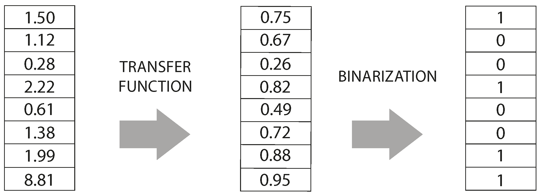
Figure 1.
Example of classic Binarization Scheme.
Figure 1.
Example of classic Binarization Scheme.
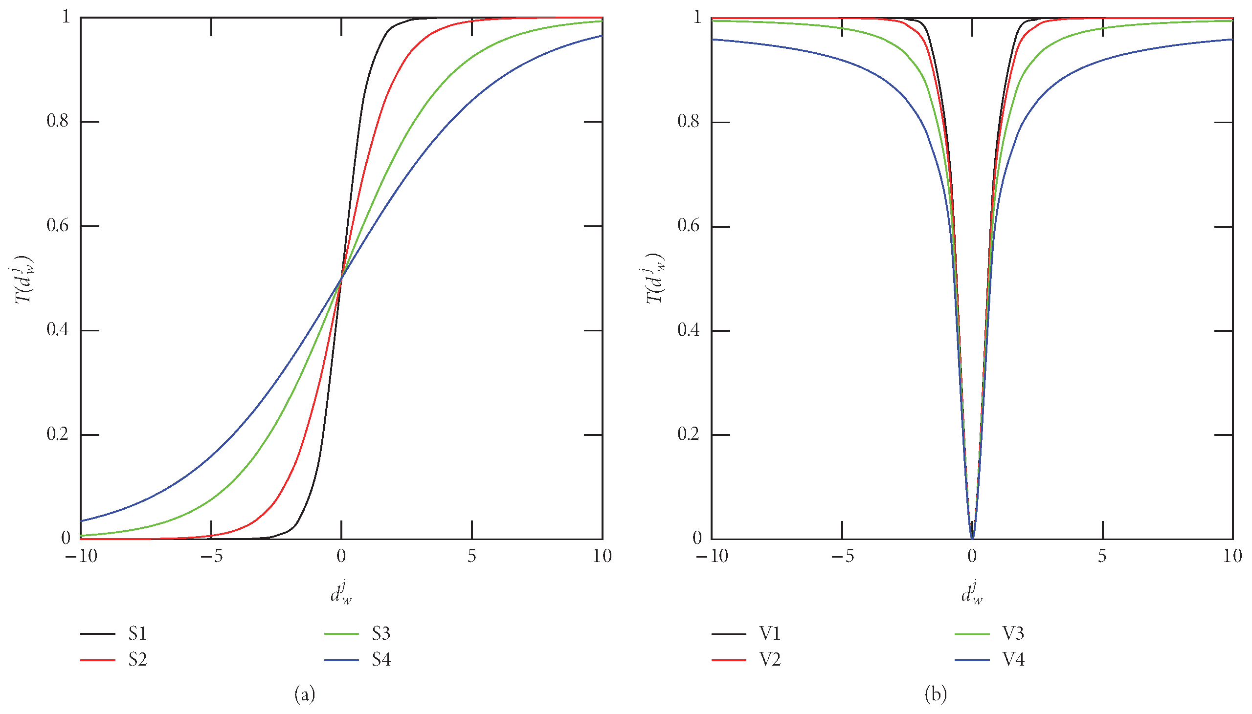
Figure 2.
(a) S and (b) V transfer functions.
Figure 2.
(a) S and (b) V transfer functions.
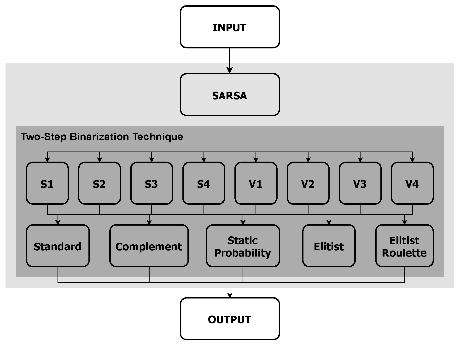
Figure 3.
Binary scheme selector with SARSA as a smart operator.
Figure 3.
Binary scheme selector with SARSA as a smart operator.
Figure 4.
A SARSA algorithm sequence.
Figure 4.
A SARSA algorithm sequence.
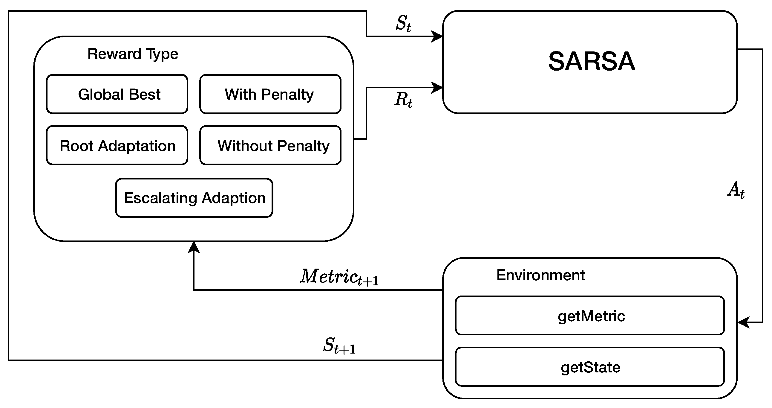
Figure 5.
A SARSA scheme for different rewards.
Figure 5.
A SARSA scheme for different rewards.
Figure 6.
WOA-SA1—The average number of actions in the exploitation state.
Figure 6.
WOA-SA1—The average number of actions in the exploitation state.
Figure 7.
WOA-SA1—The average number of actions in the exploration state.
Figure 7.
WOA-SA1—The average number of actions in the exploration state.
Figure 8.
SCA-QL5—The average number of actions in the exploitation state.
Figure 8.
SCA-QL5—The average number of actions in the exploitation state.
Figure 9.
SCA-QL5—The average number of actions in the exploration state.
Figure 9.
SCA-QL5—The average number of actions in the exploration state.
Figure 10.
GWO-QL5—The average number of actions in the exploitation state.
Figure 10.
GWO-QL5—The average number of actions in the exploitation state.
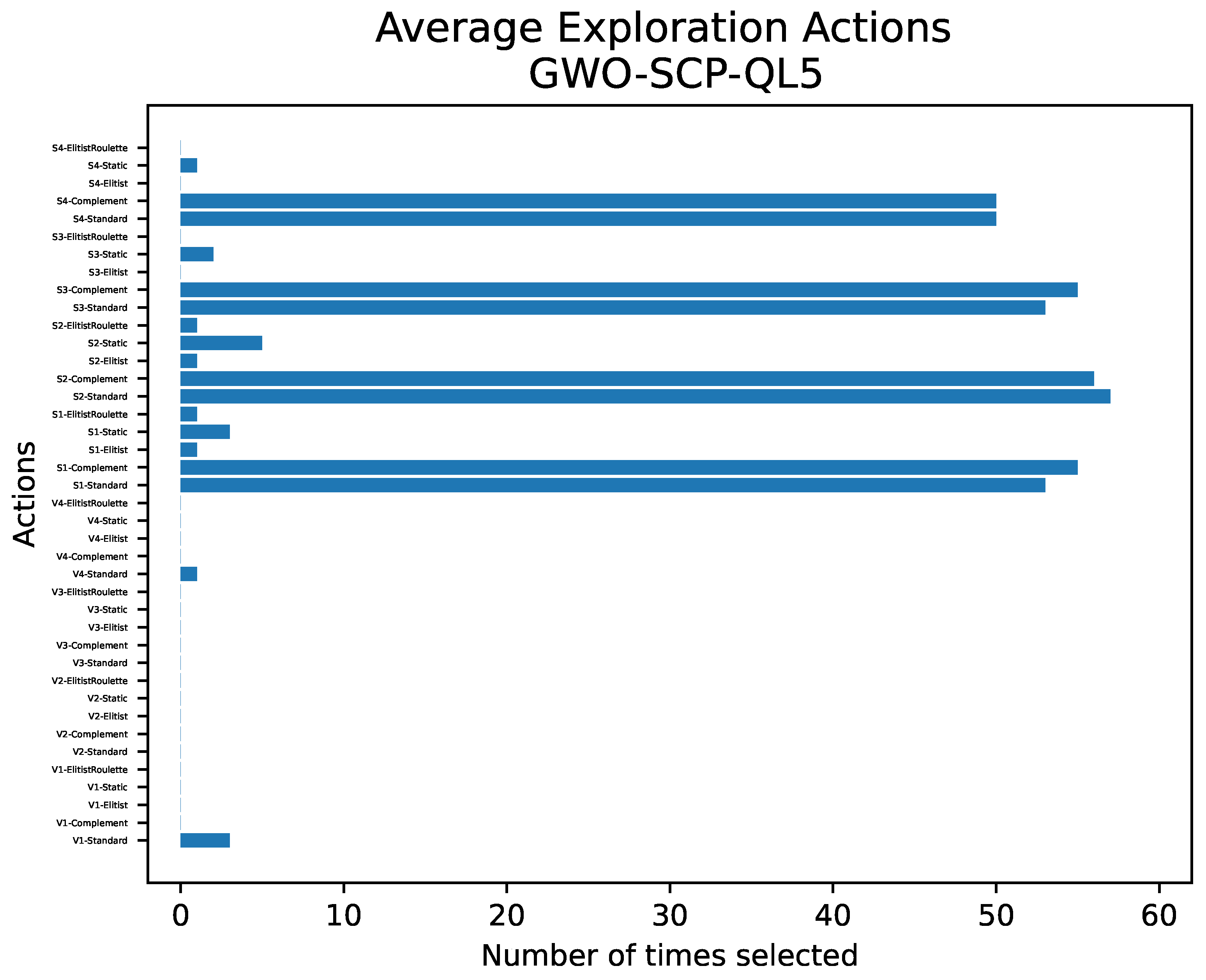
Figure 11.
GWO-QL5—The average number of actions in the exploration state.
Figure 11.
GWO-QL5—The average number of actions in the exploration state.
Figure 12.
HHO-SA1—The average number of actions in the exploitation state.
Figure 12.
HHO-SA1—The average number of actions in the exploitation state.
Figure 13.
HHO-SA1 —The average number of actions in the exploration state.
Figure 13.
HHO-SA1 —The average number of actions in the exploration state.
Figure 14.
WOA-MIR-510 Dimensional Hussain.
Figure 14.
WOA-MIR-510 Dimensional Hussain.
Figure 15.
WOA-SA1-510 Dimensional Hussain.
Figure 15.
WOA-SA1-510 Dimensional Hussain.
Figure 16.
SCA-BCL-65 Dimensional Hussain.
Figure 16.
SCA-BCL-65 Dimensional Hussain.
Figure 17.
SCA-QL5-65 Dimensional Hussain.
Figure 17.
SCA-QL5-65 Dimensional Hussain.
Figure 18.
GWO-BCL-b5 Dimensional Hussain.
Figure 18.
GWO-BCL-b5 Dimensional Hussain.
Figure 19.
GWO-QL5-b5 Dimensional Hussain.
Figure 19.
GWO-QL5-b5 Dimensional Hussain.
Figure 20.
HHO-MIR-d5 Dimensional Hussain.
Figure 20.
HHO-MIR-d5 Dimensional Hussain.
Figure 21.
HHO-SA1-d5 Dimensional Hussain.
Figure 21.
HHO-SA1-d5 Dimensional Hussain.
Figure 22.
The average Best fitness.
Figure 22.
The average Best fitness.
Figure 23.
The average Avg fitness.
Figure 23.
The average Avg fitness.
Figure 24.
The average RPD.
Figure 24.
The average RPD.
Figure 25.
The average RPD Ranking.
Figure 25.
The average RPD Ranking.
Table 1.
Transfer functions [
27].
Table 1.
Transfer functions [
27].
| Transfer Function | Type |
|---|
| S1 |
| S2 |
| S3 |
| S4 |
| V1 |
| V2 |
| V3 |
| V4 |
Table 2.
Techniques of binarization [
5].
Table 2.
Techniques of binarization [
5].
| Binarization | Type |
|---|
| Standard |
| Complement |
| Static Probability |
| Elitist |
| Elitist Roulette |
Table 3.
Reward types.
| Reward Types | Mathematical Formula |
|---|
| With Penalty | |
| Without Penalty | |
| Global Best | |
| Root Adaption | |
| Scalating Adaption | |
Table 4.
SARSA and Q-Learning implementations.
Table 4.
SARSA and Q-Learning implementations.
| Name | Reward Types |
|---|
| SA1 | With Penalty |
| SA2 | Without Penalty |
| SA3 | Global Best |
| SA4 | Root Adaption |
| SA5 | Scalating Adaption |
| QL1 | With Penalty |
| QL2 | Without Penalty |
| QL3 | Global Best |
| QL4 | Root Adaption |
| QL5 | Scalating Adaption |
Table 5.
Recommended binarization schemes in the literature.
Table 5.
Recommended binarization schemes in the literature.
| Name | Binarization | Transfer Function | Cite |
|---|
| BCL | Elitist | V4 | [29] |
| MIR | Complement | V4 | [19] |
Table 6.
Configuration details from SCP instances employed in this work.
Table 6.
Configuration details from SCP instances employed in this work.
| Instance Set | m | n | Cost Range | Density (%) |
|---|
| 4 | 200 | 1000 | [1,100] | 2 |
| 5 | 200 | 2000 | [1,100] | 2 |
| 6 | 200 | 1000 | [1,100] | 5 |
| A | 300 | 3000 | [1,100] | 2 |
| B | 300 | 3000 | [1,100] | 5 |
| C | 400 | 4000 | [1,100] | 2 |
| D | 400 | 4000 | [1,100] | 5 |
Table 7.
Result comparison with WOA employing the approaches BCL, MIR, QL1, SA1, QL2, and SA2.
Table 7.
Result comparison with WOA employing the approaches BCL, MIR, QL1, SA1, QL2, and SA2.
| | | BCL | MIR | QL1 | SA1 | QL2 | SA2 |
|---|
| Inst. | Opt. | Best | Avg | RPD | Best | Avg | RPD | Best | Avg | RPD | Best | Avg | RPD | Best | Avg | RPD | Best | Avg | RPD |
|---|
| 41 | 429 | 543 | 582.82 | 26.57 | 664 | 751.74 | 54.78 | 521 | 529.17 | 21.45 | 519 | 521.0 | 20.98 | 530 | 532.4 | 23.54 | 521 | 524.1 | 21.45 |
| 42 | 512 | 554 | 581.72 | 8.2 | 699 | 762.29 | 36.52 | 543 | 548.67 | 6.05 | 521 | 533.4 | 1.76 | 538 | 546.44 | 5.08 | 523 | 535.6 | 2.15 |
| 43 | 516 | 565 | 597.22 | 9.5 | 717 | 798.68 | 38.95 | 539 | 546.89 | 4.46 | 522 | 527.6 | 1.16 | 537 | 543.78 | 4.07 | 525 | 532.7 | 1.74 |
| 44 | 494 | 541 | 559.89 | 9.51 | 635 | 694.42 | 28.54 | 513 | 522.89 | 3.85 | 502 | 510.2 | 1.62 | 519 | 526.33 | 5.06 | 497 | 508.0 | 0.61 |
| 45 | 512 | 565 | 591.0 | 10.35 | 700 | 773.87 | 36.72 | 535 | 541.43 | 4.49 | 522 | 525.8 | 1.95 | 537 | 541.89 | 4.88 | 523 | 528.4 | 2.15 |
| 46 | 560 | 593 | 626.22 | 5.89 | 745 | 874.68 | 33.04 | 579 | 584.44 | 3.39 | 565 | 568.3 | 0.89 | 573 | 580.33 | 2.32 | 567 | 570.3 | 1.25 |
| 47 | 430 | 455 | 482.17 | 5.81 | 540 | 613.32 | 25.58 | 444 | 446.29 | 3.26 | 435 | 436.0 | 1.16 | 440 | 445.29 | 2.33 | 435 | 439.5 | 1.16 |
| 48 | 492 | 536 | 566.67 | 8.94 | 732 | 779.1 | 48.78 | 505 | 509.5 | 2.64 | 498 | 501.7 | 1.22 | 505 | 507.83 | 2.64 | 496 | 499.6 | 0.81 |
| 49 | 641 | 717 | 751.42 | 11.86 | 946 | 1013.35 | 47.58 | 680 | 689.0 | 6.08 | 658 | 672.8 | 2.65 | 686 | 690.8 | 7.02 | 671 | 677.6 | 4.68 |
| 410 | 514 | 543 | 582.82 | 5.64 | 664 | 751.74 | 29.18 | 521 | 529.17 | 1.36 | 519 | 521.0 | 0.97 | 530 | 532.4 | 3.11 | 521 | 524.1 | 1.36 |
| 51 | 253 | 288 | 298.33 | 13.83 | 369 | 416.77 | 45.85 | 276 | 277.0 | 9.09 | 266 | 271.0 | 5.14 | 277 | 278.33 | 9.49 | 267 | 273.1 | 5.53 |
| 52 | 302 | 346 | 368.33 | 14.57 | 456 | 521.03 | 50.99 | 329 | 332.83 | 8.94 | 316 | 325.7 | 4.64 | 326 | 332.17 | 7.95 | 319 | 325.3 | 5.63 |
| 53 | 226 | 240 | 251.42 | 6.19 | 323 | 351.81 | 42.92 | 232 | 233.67 | 2.65 | 229 | 229.9 | 1.33 | 232 | 233.5 | 2.65 | 230 | 230.8 | 1.77 |
| 54 | 242 | 267 | 275.67 | 10.33 | 330 | 362.45 | 36.36 | 251 | 252.67 | 3.72 | 245 | 248.0 | 1.24 | 250 | 252.5 | 3.31 | 247 | 249.4 | 2.07 |
| 55 | 211 | 223 | 236.92 | 5.69 | 274 | 294.9 | 29.86 | 217 | 218.33 | 2.84 | 213 | 214.4 | 0.95 | 216 | 218.83 | 2.37 | 212 | 214.5 | 0.47 |
| 56 | 213 | 237 | 255.08 | 11.27 | 311 | 343.97 | 46.01 | 224 | 228.33 | 5.16 | 214 | 220.4 | 0.47 | 227 | 229.0 | 6.57 | 218 | 221.3 | 2.35 |
| 57 | 293 | 330 | 337.75 | 12.63 | 403 | 450.94 | 37.54 | 306 | 311.83 | 4.44 | 296 | 300.4 | 1.02 | 311 | 313.2 | 6.14 | 302 | 304.6 | 3.07 |
| 58 | 288 | 306 | 328.43 | 6.25 | 408 | 445.03 | 41.67 | 298 | 298.5 | 3.47 | 288 | 291.6 | 0.0 | 298 | 299.33 | 3.47 | 291 | 293.9 | 1.04 |
| 59 | 279 | 307 | 322.82 | 10.04 | 403 | 443.06 | 44.44 | 287 | 289.8 | 2.87 | 281 | 283.3 | 0.72 | 284 | 287.4 | 1.79 | 282 | 284.3 | 1.08 |
| 510 | 265 | 288 | 298.33 | 8.68 | 369 | 416.77 | 39.25 | 276 | 277.0 | 4.15 | 266 | 271.0 | 0.38 | 277 | 278.33 | 4.53 | 267 | 273.1 | 0.75 |
| 61 | 138 | 161 | 170.4 | 16.67 | 336 | 368.0 | 143.48 | 143 | 147.23 | 3.62 | 141 | 142.6 | 2.17 | 144 | 146.68 | 4.35 | 141 | 144.1 | 2.17 |
| 62 | 146 | 164 | 193.55 | 12.33 | 415 | 506.68 | 184.25 | 155 | 156.17 | 6.16 | 148 | 150.8 | 1.37 | 154 | 155.83 | 5.48 | 147 | 152.3 | 0.68 |
| 63 | 145 | 172 | 194.5 | 18.62 | 390 | 474.71 | 168.97 | 149 | 150.33 | 2.76 | 145 | 147.8 | 0.0 | 149 | 150.4 | 2.76 | 147 | 148.4 | 1.38 |
| 64 | 131 | 136 | 151.0 | 3.82 | 262 | 318.9 | 100.0 | 134 | 134.83 | 2.29 | 131 | 132.3 | 0.0 | 132 | 134.17 | 0.76 | 131 | 133.1 | 0.0 |
| 65 | 161 | 188 | 209.17 | 16.77 | 379 | 514.0 | 135.4 | 178 | 181.83 | 10.56 | 161 | 167.9 | 0.0 | 180 | 181.5 | 11.8 | 163 | 172.2 | 1.24 |
| a1 | 253 | 284 | 300.8 | 12.25 | 583 | 626.6 | 130.43 | 261 | 268.38 | 3.16 | 260 | 262.3 | 2.77 | 263 | 266.84 | 3.95 | 260 | 263.2 | 2.77 |
| a2 | 252 | 284 | 306.12 | 12.7 | 553 | 615.9 | 119.44 | 271 | 271.67 | 7.54 | 255 | 262.1 | 1.19 | 266 | 269.83 | 5.56 | 261 | 264.0 | 3.57 |
| a3 | 232 | 276 | 284.75 | 18.97 | 505 | 568.9 | 117.67 | 242 | 246.5 | 4.31 | 239 | 242.8 | 3.02 | 244 | 245.6 | 5.17 | 240 | 243.4 | 3.45 |
| a4 | 234 | 282 | 308.67 | 20.51 | 518 | 568.48 | 121.37 | 245 | 249.0 | 4.7 | 238 | 242.0 | 1.71 | 251 | 251.8 | 7.26 | 238 | 242.5 | 1.71 |
| a5 | 236 | 262 | 283.88 | 11.02 | 531 | 570.32 | 125.0 | 246 | 247.5 | 4.24 | 241 | 243.2 | 2.12 | 242 | 247.33 | 2.54 | 241 | 244.2 | 2.12 |
| b1 | 69 | 90 | 104.2 | 30.43 | 549 | 592.4 | 695.65 | 71 | 71.55 | 2.9 | 69 | 69.9 | 0.0 | 70 | 71.68 | 1.45 | 69 | 70.5 | 0.0 |
| b2 | 76 | 94 | 118.25 | 23.68 | 487 | 587.03 | 540.79 | 79 | 80.0 | 3.95 | 76 | 77.0 | 0.0 | 78 | 79.5 | 2.63 | 76 | 77.2 | 0.0 |
| b3 | 80 | 110 | 134.17 | 37.5 | 662 | 766.94 | 727.5 | 82 | 82.67 | 2.5 | 81 | 81.3 | 1.25 | 82 | 82.17 | 2.5 | 81 | 81.7 | 1.25 |
| b4 | 79 | 101 | 123.92 | 27.85 | 617 | 683.74 | 681.01 | 83 | 83.83 | 5.06 | 79 | 81.2 | 0.0 | 83 | 83.83 | 5.06 | 79 | 81.3 | 0.0 |
| b5 | 72 | 82 | 116.42 | 13.89 | 521 | 603.65 | 623.61 | 73 | 73.83 | 1.39 | 72 | 72.5 | 0.0 | 73 | 74.33 | 1.39 | 72 | 72.9 | 0.0 |
| c1 | 227 | 266 | 280.4 | 17.18 | 707 | 732.6 | 211.45 | 243 | 248.27 | 7.05 | 235 | 238.2 | 3.52 | 243 | 247.81 | 7.05 | 234 | 238.4 | 3.08 |
| c2 | 219 | 264 | 280.5 | 20.55 | 703 | 799.94 | 221.0 | 236 | 239.83 | 7.76 | 225 | 230.1 | 2.74 | 234 | 238.83 | 6.85 | 229 | 232.3 | 4.57 |
| c3 | 243 | 287 | 322.2 | 18.11 | 798 | 930.16 | 228.4 | 255 | 259.67 | 4.94 | 246 | 249.4 | 1.23 | 258 | 260.83 | 6.17 | 249 | 254.2 | 2.47 |
| c4 | 219 | 261 | 283.58 | 19.18 | 721 | 788.58 | 229.22 | 232 | 233.83 | 5.94 | 221 | 226.0 | 0.91 | 232 | 233.83 | 5.94 | 227 | 229.0 | 3.65 |
| c5 | 215 | 262 | 288.83 | 21.86 | 692 | 765.71 | 221.86 | 227 | 231.0 | 5.58 | 218 | 222.0 | 1.4 | 229 | 231.33 | 6.51 | 221 | 225.4 | 2.79 |
| d1 | 60 | 99 | 135.4 | 65.0 | 781 | 869.4 | 1201.67 | 62 | 64.61 | 3.33 | 60 | 61.7 | 0.0 | 63 | 64.97 | 5.0 | 61 | 62.3 | 1.67 |
| d2 | 66 | 84 | 119.58 | 27.27 | 902 | 988.87 | 1266.67 | 69 | 69.0 | 4.55 | 67 | 67.6 | 1.52 | 68 | 69.0 | 3.03 | 67 | 67.4 | 1.52 |
| d3 | 72 | 93 | 139.58 | 29.17 | 907 | 1082.39 | 1159.72 | 77 | 78.33 | 6.94 | 74 | 75.2 | 2.78 | 76 | 77.33 | 5.56 | 73 | 74.8 | 1.39 |
| d4 | 62 | 78 | 128.5 | 25.81 | 760 | 880.65 | 1125.81 | 63 | 63.67 | 1.61 | 62 | 62.5 | 0.0 | 62 | 63.4 | 0.0 | 62 | 62.2 | 0.0 |
| d5 | 61 | 87 | 115.4 | 42.62 | 777 | 877.1 | 1173.77 | 64 | 65.17 | 4.92 | 61 | 62.4 | 0.0 | 63 | 64.33 | 3.28 | 61 | 62.6 | 0.0 |
| | | 286.91 | 310.86 | 17.01 | 572.09 | 643.15 | 276.64 | 267.02 | 270.36 | 4.94 | 259.56 | 263.21 | 1.78 | 267.38 | 270.29 | 4.9 | 260.98 | 264.66 | 2.28 |
Table 8.
Result comparison with WOA employing the approaches QL3, SA3, QL4, SA4, QL5, and SA5.
Table 8.
Result comparison with WOA employing the approaches QL3, SA3, QL4, SA4, QL5, and SA5.
| | | QL3 | SA3 | QL4 | SA4 | QL5 | SA5 |
|---|
| Inst. | Opt. | Best | Avg | RPD | Best | Avg | RPD | Best | Avg | RPD | Best | Avg | RPD | Best | Avg | RPD | Best | Avg | RPD |
|---|
| 41 | 429 | 524 | 530.0 | 22.14 | 518 | 522.4 | 20.75 | 530 | 532.5 | 23.54 | 518 | 522.8 | 20.75 | 526 | 531.64 | 22.61 | 518 | 523.6 | 20.75 |
| 42 | 512 | 543 | 548.0 | 6.05 | 528 | 534.9 | 3.12 | 534 | 544.44 | 4.3 | 525 | 534.1 | 2.54 | 524 | 547.0 | 2.34 | 525 | 536.3 | 2.54 |
| 43 | 516 | 533 | 540.33 | 3.29 | 519 | 531.8 | 0.58 | 535 | 540.78 | 3.68 | 522 | 529.8 | 1.16 | 536 | 544.11 | 3.88 | 524 | 533.5 | 1.55 |
| 44 | 494 | 516 | 524.11 | 4.45 | 502 | 508.3 | 1.62 | 513 | 524.22 | 3.85 | 504 | 511.3 | 2.02 | 517 | 525.55 | 4.66 | 508 | 514.4 | 2.83 |
| 45 | 512 | 540 | 545.78 | 5.47 | 521 | 525.8 | 1.76 | 537 | 544.78 | 4.88 | 521 | 531.0 | 1.76 | 531 | 545.0 | 3.71 | 524 | 532.6 | 2.34 |
| 46 | 560 | 577 | 583.11 | 3.04 | 568 | 570.6 | 1.43 | 577 | 584.78 | 3.04 | 563 | 569.9 | 0.54 | 573 | 582.35 | 2.32 | 566 | 571.1 | 1.07 |
| 47 | 430 | 444 | 447.14 | 3.26 | 434 | 436.8 | 0.93 | 438 | 444.67 | 1.86 | 435 | 438.7 | 1.16 | 438 | 445.0 | 1.86 | 434 | 439.0 | 0.93 |
| 48 | 492 | 506 | 510.17 | 2.85 | 497 | 500.1 | 1.02 | 505 | 509.0 | 2.64 | 495 | 500.3 | 0.61 | 504 | 508.91 | 2.44 | 495 | 501.2 | 0.61 |
| 49 | 641 | 680 | 684.25 | 6.08 | 662 | 674.6 | 3.28 | 680 | 690.0 | 6.08 | 667 | 673.1 | 4.06 | 672 | 689.04 | 4.84 | 664 | 674.1 | 3.59 |
| 410 | 514 | 524 | 530.0 | 1.95 | 518 | 522.4 | 0.78 | 530 | 532.5 | 3.11 | 518 | 522.8 | 0.78 | 526 | 531.64 | 2.33 | 518 | 523.6 | 0.78 |
| 51 | 253 | 276 | 279.33 | 9.09 | 269 | 272.8 | 6.32 | 274 | 278.0 | 8.3 | 268 | 273.1 | 5.93 | 273 | 277.48 | 7.91 | 270 | 272.3 | 6.72 |
| 52 | 302 | 330 | 332.83 | 9.27 | 319 | 324.2 | 5.63 | 327 | 331.33 | 8.28 | 317 | 324.0 | 4.97 | 325 | 331.96 | 7.62 | 319 | 324.7 | 5.63 |
| 53 | 226 | 233 | 234.5 | 3.1 | 230 | 231.8 | 1.77 | 231 | 233.67 | 2.21 | 229 | 230.5 | 1.33 | 231 | 233.96 | 2.21 | 229 | 230.4 | 1.33 |
| 54 | 242 | 246 | 250.0 | 1.65 | 246 | 249.2 | 1.65 | 250 | 251.5 | 3.31 | 247 | 249.8 | 2.07 | 249 | 252.35 | 2.89 | 247 | 250.0 | 2.07 |
| 55 | 211 | 218 | 219.33 | 3.32 | 213 | 215.3 | 0.95 | 217 | 218.33 | 2.84 | 212 | 215.7 | 0.47 | 215 | 218.22 | 1.9 | 212 | 215.4 | 0.47 |
| 56 | 213 | 225 | 227.0 | 5.63 | 215 | 222.2 | 0.94 | 228 | 229.5 | 7.04 | 218 | 220.8 | 2.35 | 223 | 228.04 | 4.69 | 218 | 221.0 | 2.35 |
| 57 | 293 | 307 | 310.2 | 4.78 | 301 | 304.0 | 2.73 | 303 | 311.0 | 3.41 | 298 | 303.3 | 1.71 | 307 | 311.81 | 4.78 | 302 | 306.4 | 3.07 |
| 58 | 288 | 297 | 298.0 | 3.12 | 291 | 292.7 | 1.04 | 295 | 297.83 | 2.43 | 289 | 293.5 | 0.35 | 294 | 297.87 | 2.08 | 290 | 292.8 | 0.69 |
| 59 | 279 | 284 | 289.17 | 1.79 | 281 | 284.8 | 0.72 | 287 | 290.5 | 2.87 | 282 | 283.6 | 1.08 | 284 | 289.57 | 1.79 | 281 | 284.8 | 0.72 |
| 510 | 265 | 276 | 279.33 | 4.15 | 269 | 272.8 | 1.51 | 274 | 278.0 | 3.4 | 268 | 273.1 | 1.13 | 273 | 277.48 | 3.02 | 270 | 272.3 | 1.89 |
| 61 | 138 | 144 | 146.74 | 4.35 | 141 | 143.5 | 2.17 | 142 | 146.39 | 2.9 | 142 | 143.8 | 2.9 | 143 | 146.61 | 3.62 | 142 | 143.9 | 2.9 |
| 62 | 146 | 152 | 156.0 | 4.11 | 148 | 153.3 | 1.37 | 156 | 157.33 | 6.85 | 149 | 152.3 | 2.05 | 154 | 156.65 | 5.48 | 150 | 152.9 | 2.74 |
| 63 | 145 | 148 | 149.17 | 2.07 | 148 | 149.0 | 2.07 | 149 | 150.33 | 2.76 | 146 | 147.9 | 0.69 | 147 | 149.96 | 1.38 | 147 | 148.4 | 1.38 |
| 64 | 131 | 134 | 134.67 | 2.29 | 131 | 132.9 | 0.0 | 131 | 134.5 | 0.0 | 131 | 133.1 | 0.0 | 133 | 135.04 | 1.53 | 132 | 133.9 | 0.76 |
| 65 | 161 | 176 | 179.5 | 9.32 | 168 | 174.5 | 4.35 | 177 | 179.17 | 9.94 | 164 | 170.7 | 1.86 | 175 | 180.0 | 8.7 | 165 | 172.9 | 2.48 |
| a1 | 253 | 264 | 266.97 | 4.35 | 261 | 263.7 | 3.16 | 264 | 266.87 | 4.35 | 261 | 263.4 | 3.16 | 264 | 267.22 | 4.35 | 260 | 263.2 | 2.77 |
| a2 | 252 | 265 | 270.4 | 5.16 | 260 | 265.1 | 3.17 | 269 | 271.0 | 6.75 | 261 | 264.6 | 3.57 | 266 | 270.83 | 5.56 | 259 | 264.1 | 2.78 |
| a3 | 232 | 242 | 246.0 | 4.31 | 240 | 242.1 | 3.45 | 243 | 245.5 | 4.74 | 241 | 242.7 | 3.88 | 240 | 246.17 | 3.45 | 240 | 243.4 | 3.45 |
| a4 | 234 | 246 | 246.6 | 5.13 | 240 | 243.1 | 2.56 | 249 | 250.0 | 6.41 | 238 | 242.8 | 1.71 | 244 | 249.04 | 4.27 | 240 | 244.1 | 2.56 |
| a5 | 236 | 241 | 248.17 | 2.12 | 241 | 244.4 | 2.12 | 246 | 248.17 | 4.24 | 240 | 242.5 | 1.69 | 243 | 248.74 | 2.97 | 241 | 244.4 | 2.12 |
| b1 | 69 | 70 | 71.87 | 1.45 | 69 | 70.3 | 0.0 | 69 | 71.68 | 0.0 | 69 | 70.6 | 0.0 | 71 | 71.65 | 2.9 | 69 | 69.9 | 0.0 |
| b2 | 76 | 78 | 79.17 | 2.63 | 76 | 77.0 | 0.0 | 78 | 79.5 | 2.63 | 76 | 77.3 | 0.0 | 78 | 79.87 | 2.63 | 76 | 77.0 | 0.0 |
| b3 | 80 | 82 | 82.67 | 2.5 | 81 | 81.4 | 1.25 | 82 | 82.0 | 2.5 | 81 | 81.6 | 1.25 | 81 | 82.26 | 1.25 | 81 | 81.5 | 1.25 |
| b4 | 79 | 83 | 83.5 | 5.06 | 80 | 81.9 | 1.27 | 83 | 84.0 | 5.06 | 80 | 81.6 | 1.27 | 83 | 83.87 | 5.06 | 80 | 81.4 | 1.27 |
| b5 | 72 | 74 | 74.5 | 2.78 | 72 | 73.0 | 0.0 | 73 | 74.33 | 1.39 | 72 | 73.1 | 0.0 | 73 | 74.18 | 1.39 | 72 | 73.0 | 0.0 |
| c1 | 227 | 241 | 247.48 | 6.17 | 233 | 239.6 | 2.64 | 241 | 247.29 | 6.17 | 236 | 241.0 | 3.96 | 243 | 247.75 | 7.05 | 237 | 240.6 | 4.41 |
| c2 | 219 | 238 | 240.17 | 8.68 | 230 | 233.3 | 5.02 | 238 | 239.6 | 8.68 | 229 | 232.5 | 4.57 | 232 | 239.81 | 5.94 | 229 | 232.4 | 4.57 |
| c3 | 243 | 261 | 261.8 | 7.41 | 248 | 253.4 | 2.06 | 258 | 261.33 | 6.17 | 248 | 253.9 | 2.06 | 256 | 260.61 | 5.35 | 247 | 251.8 | 1.65 |
| c4 | 219 | 228 | 234.17 | 4.11 | 226 | 229.2 | 3.2 | 230 | 233.5 | 5.02 | 223 | 227.4 | 1.83 | 229 | 233.09 | 4.57 | 227 | 229.4 | 3.65 |
| c5 | 215 | 229 | 231.0 | 6.51 | 221 | 224.0 | 2.79 | 223 | 228.67 | 3.72 | 222 | 224.8 | 3.26 | 226 | 231.0 | 5.12 | 222 | 224.7 | 3.26 |
| d1 | 60 | 64 | 65.06 | 6.67 | 61 | 62.7 | 1.67 | 64 | 64.79 | 6.67 | 61 | 62.2 | 1.67 | 64 | 65.13 | 6.67 | 61 | 62.6 | 1.67 |
| d2 | 66 | 67 | 68.75 | 1.52 | 66 | 67.4 | 0.0 | 68 | 68.83 | 3.03 | 67 | 67.8 | 1.52 | 68 | 69.04 | 3.03 | 67 | 67.8 | 1.52 |
| d3 | 72 | 76 | 77.33 | 5.56 | 74 | 75.6 | 2.78 | 76 | 77.33 | 5.56 | 73 | 75.0 | 1.39 | 77 | 77.7 | 6.94 | 74 | 75.8 | 2.78 |
| d4 | 62 | 63 | 63.8 | 1.61 | 62 | 62.6 | 0.0 | 63 | 63.67 | 1.61 | 62 | 62.1 | 0.0 | 62 | 63.43 | 0.0 | 62 | 62.4 | 0.0 |
| d5 | 61 | 63 | 65.0 | 3.28 | 62 | 62.5 | 1.64 | 65 | 65.67 | 6.56 | 61 | 62.9 | 0.0 | 63 | 65.3 | 3.28 | 61 | 62.2 | 0.0 |
| | | 266.84 | 277 | 4.75 | 260.89 | 264.51 | 2.38 | 266.71 | 270.2 | 4.77 | 260.64 | 264.42 | 2.25 | 265.24 | 270.31 | 4.27 | 261.22 | 264.96 | 2.49 |
Table 9.
Result comparison with SCA employing the approaches BCL, MIR, QL1, SA1, QL2, and SA2.
Table 9.
Result comparison with SCA employing the approaches BCL, MIR, QL1, SA1, QL2, and SA2.
| | | BCL | MIR | QL1 | SA1 | QL2 | SA2 |
|---|
| Inst. | Opt. | Best | Avg | RPD | Best | Avg | RPD | Best | Avg | RPD | Best | Avg | RPD | Best | Avg | RPD | Best | Avg | RPD |
|---|
| 41 | 429 | 557 | 580.0 | 29.84 | 545 | 734.48 | 27.04 | 533 | 538.0 | 24.24 | 515 | 520.93 | 20.05 | 530 | 537.83 | 23.54 | 516 | 519.2 | 20.28 |
| 42 | 512 | 573 | 605.78 | 11.91 | 550 | 725.1 | 7.42 | 548 | 552.89 | 7.03 | 524 | 531.38 | 2.34 | 537 | 551.11 | 4.88 | 527 | 535.9 | 2.93 |
| 43 | 516 | 557 | 598.83 | 7.95 | 559 | 766.84 | 8.33 | 548 | 552.67 | 6.2 | 524 | 529.0 | 1.55 | 543 | 554.44 | 5.23 | 524 | 529.0 | 1.55 |
| 44 | 494 | 533 | 557.06 | 7.89 | 547 | 688.48 | 10.73 | 519 | 531.22 | 5.06 | 500 | 510.38 | 1.21 | 530 | 533.78 | 7.29 | 502 | 514.2 | 1.62 |
| 45 | 512 | 563 | 591.5 | 9.96 | 565 | 751.35 | 10.35 | 540 | 549.22 | 5.47 | 518 | 527.69 | 1.17 | 537 | 551.67 | 4.88 | 524 | 530.3 | 2.34 |
| 46 | 560 | 594 | 635.22 | 6.07 | 591 | 840.42 | 5.54 | 578 | 587.33 | 3.21 | 564 | 568.1 | 0.71 | 577 | 589.89 | 3.04 | 564 | 571.45 | 0.71 |
| 47 | 430 | 449 | 483.44 | 4.42 | 456 | 586.97 | 6.05 | 440 | 448.11 | 2.33 | 434 | 439.5 | 0.93 | 442 | 448.25 | 2.79 | 435 | 440.1 | 1.16 |
| 48 | 492 | 515 | 565.67 | 4.67 | 518 | 727.23 | 5.28 | 507 | 514.6 | 3.05 | 494 | 498.25 | 0.41 | 512 | 516.0 | 4.07 | 497 | 501.9 | 1.02 |
| 49 | 641 | 713 | 759.75 | 11.23 | 698 | 964.68 | 8.89 | 689 | 695.67 | 7.49 | 657 | 674.0 | 2.5 | 696 | 700.83 | 8.58 | 665 | 676.9 | 3.74 |
| 410 | 514 | 557 | 580.0 | 8.37 | 545 | 734.48 | 6.03 | 533 | 538.0 | 3.7 | 515 | 520.93 | 0.19 | 530 | 537.83 | 3.11 | 516 | 519.2 | 0.39 |
| 51 | 253 | 289 | 303.33 | 14.23 | 282 | 396.55 | 11.46 | 276 | 281.0 | 9.09 | 270 | 272.83 | 6.72 | 279 | 282.17 | 10.28 | 270 | 272.8 | 6.72 |
| 52 | 302 | 346 | 366.92 | 14.57 | 335 | 486.87 | 10.93 | 333 | 334.5 | 10.26 | 316 | 322.83 | 4.64 | 334 | 336.0 | 10.6 | 318 | 326.27 | 5.3 |
| 53 | 226 | 246 | 258.17 | 8.85 | 238 | 331.74 | 5.31 | 233 | 235.5 | 3.1 | 230 | 230.91 | 1.77 | 231 | 235.67 | 2.21 | 230 | 231.1 | 1.77 |
| 54 | 242 | 257 | 276.5 | 6.2 | 253 | 338.84 | 4.55 | 255 | 256.0 | 5.37 | 247 | 249.33 | 2.07 | 253 | 255.67 | 4.55 | 247 | 250.5 | 2.07 |
| 55 | 211 | 227 | 237.92 | 7.58 | 226 | 289.03 | 7.11 | 216 | 221.0 | 2.37 | 213 | 215.18 | 0.95 | 218 | 221.0 | 3.32 | 213 | 216.36 | 0.95 |
| 56 | 213 | 244 | 258.58 | 14.55 | 234 | 324.77 | 9.86 | 223 | 230.67 | 4.69 | 214 | 220.15 | 0.47 | 221 | 230.17 | 3.76 | 218 | 221.8 | 2.35 |
| 57 | 293 | 323 | 342.75 | 10.24 | 313 | 427.1 | 6.83 | 317 | 319.6 | 8.19 | 296 | 303.83 | 1.02 | 310 | 314.4 | 5.8 | 297 | 305.27 | 1.37 |
| 58 | 288 | 320 | 333.3 | 11.11 | 302 | 444.35 | 4.86 | 298 | 299.33 | 3.47 | 291 | 294.18 | 1.04 | 300 | 301.8 | 4.17 | 290 | 294.55 | 0.69 |
| 59 | 279 | 312 | 326.92 | 11.83 | 298 | 414.26 | 6.81 | 290 | 293.67 | 3.94 | 281 | 285.18 | 0.72 | 291 | 294.4 | 4.3 | 283 | 284.7 | 1.43 |
| 510 | 265 | 289 | 303.33 | 9.06 | 282 | 396.55 | 6.42 | 276 | 281.0 | 4.15 | 270 | 272.83 | 1.89 | 279 | 282.17 | 5.28 | 270 | 272.8 | 1.89 |
| 61 | 138 | 152 | 165.2 | 10.14 | 348 | 369.8 | 152.17 | 141 | 145.77 | 2.17 | 142 | 145.45 | 2.9 | 144 | 148.16 | 4.35 | 142 | 145.36 | 2.9 |
| 62 | 146 | 170 | 196.17 | 16.44 | 161 | 484.97 | 10.27 | 157 | 159.83 | 7.53 | 146 | 152.63 | 0.0 | 158 | 159.83 | 8.22 | 151 | 153.0 | 3.42 |
| 63 | 145 | 156 | 179.75 | 7.59 | 151 | 436.71 | 4.14 | 149 | 151.33 | 2.76 | 145 | 150.65 | 0.0 | 150 | 151.67 | 3.45 | 148 | 149.5 | 2.07 |
| 64 | 131 | 139 | 155.25 | 6.11 | 137 | 303.0 | 4.58 | 135 | 136.33 | 3.05 | 131 | 133.53 | 0.0 | 136 | 136.17 | 3.82 | 131 | 133.6 | 0.0 |
| 65 | 161 | 193 | 215.25 | 19.88 | 185 | 450.06 | 14.91 | 177 | 183.17 | 9.94 | 161 | 169.72 | 0.0 | 178 | 183.67 | 10.56 | 165 | 171.82 | 2.48 |
| a1 | 253 | 286 | 302.8 | 13.04 | 272 | 596.8 | 7.51 | 262 | 267.13 | 3.56 | 261 | 264.73 | 3.16 | 266 | 269.42 | 5.14 | 260 | 263.9 | 2.77 |
| a2 | 252 | 289 | 304.2 | 14.68 | 281 | 577.52 | 11.51 | 271 | 273.83 | 7.54 | 258 | 264.82 | 2.38 | 272 | 273.67 | 7.94 | 254 | 266.2 | 0.79 |
| a3 | 232 | 266 | 283.44 | 14.66 | 250 | 555.52 | 7.76 | 245 | 248.6 | 5.6 | 242 | 259.5 | 4.31 | 246 | 249.0 | 6.03 | 238 | 245.5 | 2.59 |
| a4 | 234 | 271 | 289.3 | 15.81 | 256 | 544.71 | 9.4 | 250 | 253.0 | 6.84 | 239 | 247.91 | 2.14 | 248 | 253.6 | 5.98 | 241 | 246.3 | 2.99 |
| a5 | 236 | 266 | 286.86 | 12.71 | 253 | 513.9 | 7.2 | 249 | 250.67 | 5.51 | 243 | 249.64 | 2.97 | 248 | 252.83 | 5.08 | 242 | 244.6 | 2.54 |
| b1 | 69 | 81 | 108.6 | 17.39 | 527 | 585.0 | 663.77 | 70 | 71.74 | 1.45 | 69 | 99.0 | 0.0 | 71 | 72.68 | 2.9 | 69 | 70.9 | 0.0 |
| b2 | 76 | 93 | 110.33 | 22.37 | 81 | 529.32 | 6.58 | 78 | 80.33 | 2.63 | 76 | 79.53 | 0.0 | 80 | 82.0 | 5.26 | 76 | 77.8 | 0.0 |
| b3 | 80 | 90 | 117.08 | 12.5 | 84 | 687.06 | 5.0 | 82 | 83.33 | 2.5 | 81 | 82.84 | 1.25 | 83 | 83.83 | 3.75 | 80 | 84.4 | 0.0 |
| b4 | 79 | 96 | 116.42 | 21.52 | 84 | 582.87 | 6.33 | 83 | 84.0 | 5.06 | 80 | 86.13 | 1.27 | 83 | 84.83 | 5.06 | 82 | 83.3 | 3.8 |
| b5 | 72 | 83 | 104.09 | 15.28 | 75 | 573.1 | 4.17 | 74 | 75.0 | 2.78 | 72 | 75.53 | 0.0 | 75 | 75.33 | 4.17 | 72 | 74.27 | 0.0 |
| c1 | 227 | 269 | 302.8 | 18.5 | 254 | 536.6 | 11.89 | 240 | 245.55 | 5.73 | 235 | 241.1 | 3.52 | 241 | 251.32 | 6.17 | 237 | 240.5 | 4.41 |
| c2 | 219 | 264 | 284.0 | 20.55 | 243 | 715.52 | 10.96 | 235 | 242.5 | 7.31 | 226 | 236.58 | 3.2 | 241 | 244.17 | 10.05 | 230 | 235.7 | 5.02 |
| c3 | 243 | 273 | 306.25 | 12.35 | 265 | 745.74 | 9.05 | 261 | 263.17 | 7.41 | 248 | 258.7 | 2.06 | 259 | 263.17 | 6.58 | 252 | 254.5 | 3.7 |
| c4 | 219 | 251 | 280.67 | 14.61 | 235 | 669.42 | 7.31 | 236 | 237.0 | 7.76 | 225 | 243.67 | 2.74 | 233 | 235.83 | 6.39 | 228 | 231.6 | 4.11 |
| c5 | 215 | 239 | 271.17 | 11.16 | 232 | 569.45 | 7.91 | 228 | 232.33 | 6.05 | 218 | 226.33 | 1.4 | 233 | 234.33 | 8.37 | 222 | 225.9 | 3.26 |
| d1 | 60 | 89 | 93.2 | 48.33 | 67 | 701.4 | 11.67 | 62 | 64.42 | 3.33 | 61 | 67.62 | 1.67 | 64 | 66.0 | 6.67 | 62 | 64.6 | 3.33 |
| d2 | 66 | 81 | 105.83 | 22.73 | 69 | 802.45 | 4.55 | 69 | 70.33 | 4.55 | 67 | 71.35 | 1.52 | 69 | 69.5 | 4.55 | 67 | 73.27 | 1.52 |
| d3 | 72 | 81 | 109.75 | 12.5 | 79 | 845.29 | 9.72 | 78 | 78.67 | 8.33 | 74 | 77.17 | 2.78 | 78 | 79.0 | 8.33 | 75 | 81.8 | 4.17 |
| d4 | 62 | 68 | 91.42 | 9.68 | 64 | 675.35 | 3.23 | 63 | 64.0 | 1.61 | 62 | 74.31 | 0.0 | 63 | 64.5 | 1.61 | 62 | 64.6 | 0.0 |
| d5 | 61 | 77 | 101.0 | 26.23 | 67 | 767.1 | 9.84 | 65 | 66.6 | 6.56 | 61 | 67.4 | 0.0 | 66 | 67.0 | 8.2 | 62 | 69.27 | 1.64 |
| | | 284.16 | 307.68 | 13.94 | 290.16 | 581.97 | 26.03 | 269.16 | 273.08 | 5.55 | 259.91 | 266.96 | 2.04 | 269.67 | 273.92 | 6.01 | 261.2 | 265.92 | 2.62 |
Table 10.
Result comparison with SCA employing the approaches QL3, SA3, QL4, SA4, QL5, and SA5.
Table 10.
Result comparison with SCA employing the approaches QL3, SA3, QL4, SA4, QL5, and SA5.
| | | QL3 | SA3 | QL4 | SA4 | QL5 | SA5 |
|---|
| Inst. | Opt. | Best | Avg | RPD | Best | Avg | RPD | Best | Avg | RPD | Best | Avg | RPD | Best | Avg | RPD | Best | Avg | RPD |
|---|
| 41 | 429 | 534 | 537.5 | 24.48 | 517 | 521.85 | 20.51 | 533 | 536.83 | 24.24 | 518 | 523.75 | 20.75 | 530 | 535.17 | 23.54 | 518 | 522.32 | 20.75 |
| 42 | 512 | 547 | 552.67 | 6.84 | 524 | 533.64 | 2.34 | 552 | 556.89 | 7.81 | 526 | 534.3 | 2.73 | 537 | 552.37 | 4.88 | 521 | 534.52 | 1.76 |
| 43 | 516 | 540 | 555.0 | 4.65 | 522 | 529.42 | 1.16 | 535 | 550.22 | 3.68 | 524 | 534.17 | 1.55 | 536 | 547.05 | 3.88 | 523 | 531.2 | 1.36 |
| 44 | 494 | 518 | 531.33 | 4.86 | 500 | 510.57 | 1.21 | 512 | 532.56 | 3.64 | 501 | 509.08 | 1.42 | 511 | 532.84 | 3.44 | 499 | 510.43 | 1.01 |
| 45 | 512 | 544 | 552.56 | 6.25 | 520 | 526.2 | 1.56 | 541 | 552.67 | 5.66 | 526 | 531.6 | 2.73 | 542 | 549.79 | 5.86 | 522 | 529.45 | 1.95 |
| 46 | 560 | 577 | 588.22 | 3.04 | 567 | 571.79 | 1.25 | 584 | 592.56 | 4.29 | 566 | 571.0 | 1.07 | 568 | 589.3 | 1.43 | 565 | 569.58 | 0.89 |
| 47 | 430 | 447 | 450.5 | 3.95 | 434 | 437.62 | 0.93 | 447 | 452.88 | 3.95 | 434 | 438.58 | 0.93 | 439 | 451.95 | 2.09 | 434 | 438.13 | 0.93 |
| 48 | 492 | 509 | 513.0 | 3.46 | 494 | 500.42 | 0.41 | 508 | 515.83 | 3.25 | 496 | 502.3 | 0.81 | 507 | 515.04 | 3.05 | 493 | 499.67 | 0.2 |
| 49 | 641 | 692 | 696.83 | 7.96 | 664 | 678.69 | 3.59 | 688 | 694.83 | 7.33 | 666 | 674.31 | 3.9 | 684 | 698.48 | 6.71 | 658 | 672.58 | 2.65 |
| 410 | 514 | 534 | 537.5 | 3.89 | 517 | 521.85 | 0.58 | 533 | 536.83 | 3.7 | 518 | 523.75 | 0.78 | 530 | 535.17 | 3.11 | 518 | 522.32 | 0.78 |
| 51 | 253 | 277 | 282.5 | 9.49 | 268 | 271.92 | 5.93 | 278 | 282.33 | 9.88 | 267 | 274.73 | 5.53 | 274 | 282.39 | 8.3 | 270 | 273.52 | 6.72 |
| 52 | 302 | 332 | 336.5 | 9.93 | 322 | 327.62 | 6.62 | 328 | 334.5 | 8.61 | 320 | 326.4 | 5.96 | 329 | 336.28 | 8.94 | 313 | 324.5 | 3.64 |
| 53 | 226 | 235 | 236.17 | 3.98 | 230 | 230.54 | 1.77 | 236 | 236.83 | 4.42 | 230 | 231.18 | 1.77 | 230 | 236.13 | 1.77 | 229 | 231.1 | 1.33 |
| 54 | 242 | 253 | 255.17 | 4.55 | 248 | 249.91 | 2.48 | 252 | 256.17 | 4.13 | 246 | 250.0 | 1.65 | 251 | 254.96 | 3.72 | 243 | 249.14 | 0.41 |
| 55 | 211 | 218 | 222.33 | 3.32 | 212 | 215.92 | 0.47 | 221 | 222.0 | 4.74 | 212 | 215.69 | 0.47 | 217 | 221.09 | 2.84 | 212 | 215.43 | 0.47 |
| 56 | 213 | 231 | 232.8 | 8.45 | 213 | 221.27 | 0.0 | 228 | 233.2 | 7.04 | 218 | 222.45 | 2.35 | 224 | 231.2 | 5.16 | 217 | 222.22 | 1.88 |
| 57 | 293 | 313 | 317.33 | 6.83 | 298 | 303.75 | 1.71 | 317 | 321.17 | 8.19 | 297 | 304.08 | 1.37 | 314 | 317.84 | 7.17 | 296 | 303.68 | 1.02 |
| 58 | 288 | 298 | 301.83 | 3.47 | 291 | 294.91 | 1.04 | 298 | 300.0 | 3.47 | 290 | 295.55 | 0.69 | 297 | 301.39 | 3.12 | 289 | 293.0 | 0.35 |
| 59 | 279 | 289 | 293.5 | 3.58 | 281 | 286.91 | 0.72 | 292 | 293.67 | 4.66 | 280 | 284.0 | 0.36 | 286 | 293.17 | 2.51 | 281 | 284.82 | 0.72 |
| 510 | 265 | 277 | 282.5 | 4.53 | 268 | 271.92 | 1.13 | 278 | 282.33 | 4.91 | 267 | 274.73 | 0.75 | 274 | 282.39 | 3.4 | 270 | 273.52 | 1.89 |
| 61 | 138 | 144 | 148.42 | 4.35 | 141 | 143.88 | 2.17 | 146 | 148.29 | 5.8 | 141 | 144.42 | 2.17 | 146 | 148.65 | 5.8 | 141 | 144.72 | 2.17 |
| 62 | 146 | 157 | 159.17 | 7.53 | 148 | 152.0 | 1.37 | 155 | 158.0 | 6.16 | 150 | 153.83 | 2.74 | 154 | 158.26 | 5.48 | 149 | 152.25 | 2.05 |
| 63 | 145 | 151 | 151.83 | 4.14 | 148 | 149.38 | 2.07 | 150 | 151.67 | 3.45 | 148 | 150.14 | 2.07 | 149 | 151.65 | 2.76 | 145 | 148.52 | 0.0 |
| 64 | 131 | 134 | 135.67 | 2.29 | 131 | 134.14 | 0.0 | 135 | 136.2 | 3.05 | 131 | 134.38 | 0.0 | 134 | 136.52 | 2.29 | 131 | 133.86 | 0.0 |
| 65 | 161 | 182 | 183.67 | 13.04 | 162 | 170.92 | 0.62 | 179 | 183.17 | 11.18 | 161 | 171.83 | 0.0 | 175 | 182.96 | 8.7 | 163 | 170.43 | 1.24 |
| a1 | 253 | 263 | 268.81 | 3.95 | 260 | 263.5 | 2.77 | 263 | 268.9 | 3.95 | 262 | 265.18 | 3.56 | 265 | 269.68 | 4.74 | 262 | 264.44 | 3.56 |
| a2 | 252 | 273 | 275.0 | 8.33 | 263 | 266.36 | 4.37 | 271 | 272.83 | 7.54 | 262 | 267.4 | 3.97 | 270 | 274.33 | 7.14 | 261 | 265.59 | 3.57 |
| a3 | 232 | 249 | 252.0 | 7.33 | 241 | 243.36 | 3.88 | 251 | 251.33 | 8.19 | 242 | 247.0 | 4.31 | 242 | 248.74 | 4.31 | 240 | 243.18 | 3.45 |
| a4 | 234 | 249 | 252.2 | 6.41 | 240 | 243.1 | 2.56 | 250 | 252.2 | 6.84 | 237 | 243.64 | 1.28 | 247 | 253.5 | 5.56 | 240 | 244.82 | 2.56 |
| a5 | 236 | 245 | 250.33 | 3.81 | 242 | 244.4 | 2.54 | 247 | 251.5 | 4.66 | 243 | 246.1 | 2.97 | 248 | 251.22 | 5.08 | 241 | 244.44 | 2.12 |
| b1 | 69 | 72 | 72.9 | 4.35 | 69 | 72.07 | 0.0 | 72 | 72.87 | 4.35 | 69 | 70.42 | 0.0 | 72 | 73.03 | 4.35 | 69 | 72.8 | 0.0 |
| b2 | 76 | 80 | 81.5 | 5.26 | 76 | 77.75 | 0.0 | 78 | 80.67 | 2.63 | 76 | 80.54 | 0.0 | 78 | 81.39 | 2.63 | 76 | 77.68 | 0.0 |
| b3 | 80 | 82 | 83.67 | 2.5 | 81 | 82.5 | 1.25 | 82 | 84.0 | 2.5 | 81 | 82.07 | 1.25 | 81 | 83.35 | 1.25 | 81 | 81.58 | 1.25 |
| b4 | 79 | 82 | 84.33 | 3.8 | 81 | 82.93 | 2.53 | 83 | 84.83 | 5.06 | 81 | 83.91 | 2.53 | 84 | 85.26 | 6.33 | 79 | 82.43 | 0.0 |
| b5 | 72 | 74 | 74.83 | 2.78 | 72 | 75.92 | 0.0 | 74 | 75.0 | 2.78 | 72 | 74.25 | 0.0 | 74 | 74.78 | 2.78 | 72 | 74.38 | 0.0 |
| c1 | 227 | 244 | 251.03 | 7.49 | 234 | 239.09 | 3.08 | 239 | 251.0 | 5.29 | 234 | 237.5 | 3.08 | 244 | 250.94 | 7.49 | 237 | 242.5 | 4.41 |
| c2 | 219 | 241 | 243.33 | 10.05 | 229 | 231.93 | 4.57 | 236 | 241.8 | 7.76 | 225 | 231.75 | 2.74 | 236 | 242.17 | 7.76 | 226 | 232.41 | 3.2 |
| c3 | 243 | 260 | 262.8 | 7.0 | 247 | 253.09 | 1.65 | 259 | 262.83 | 6.58 | 252 | 260.1 | 3.7 | 256 | 263.87 | 5.35 | 248 | 255.41 | 2.06 |
| c4 | 219 | 236 | 237.83 | 7.76 | 227 | 233.82 | 3.65 | 234 | 236.67 | 6.85 | 225 | 235.31 | 2.74 | 234 | 237.13 | 6.85 | 225 | 231.59 | 2.74 |
| c5 | 215 | 232 | 233.83 | 7.91 | 222 | 225.0 | 3.26 | 227 | 231.83 | 5.58 | 219 | 224.71 | 1.86 | 226 | 233.62 | 5.12 | 221 | 225.47 | 2.79 |
| d1 | 60 | 64 | 66.0 | 6.67 | 61 | 63.73 | 1.67 | 64 | 65.81 | 6.67 | 61 | 64.08 | 1.67 | 63 | 66.06 | 5.0 | 60 | 64.16 | 0.0 |
| d2 | 66 | 69 | 69.8 | 4.55 | 67 | 71.27 | 1.52 | 69 | 70.0 | 4.55 | 67 | 70.42 | 1.52 | 68 | 70.13 | 3.03 | 67 | 69.14 | 1.52 |
| d3 | 72 | 78 | 79.0 | 8.33 | 73 | 77.27 | 1.39 | 78 | 79.33 | 8.33 | 73 | 80.17 | 1.39 | 78 | 79.09 | 8.33 | 73 | 78.0 | 1.39 |
| d4 | 62 | 63 | 63.83 | 1.61 | 62 | 65.3 | 0.0 | 64 | 64.4 | 3.23 | 62 | 64.73 | 0.0 | 63 | 64.3 | 1.61 | 62 | 64.15 | 0.0 |
| d5 | 61 | 64 | 66.17 | 4.92 | 61 | 67.14 | 0.0 | 65 | 65.83 | 6.56 | 61 | 64.6 | 0.0 | 64 | 66.35 | 4.92 | 61 | 64.74 | 0.0 |
| | | 277 | 273.86 | 6.08 | 260.62 | 265.26 | 2.27 | 269.6 | 273.89 | 5.94 | 260.82 | 266.0 | 2.29 | 267.36 | 273.58 | 5.1 | 262 | 265.11 | 2.02 |
Table 11.
Result comparison with GWO employing the approaches BCL, MIR, QL1, SA1, QL2, and SA2.
Table 11.
Result comparison with GWO employing the approaches BCL, MIR, QL1, SA1, QL2, and SA2.
| | | BCL | MIR | QL1 | SA1 | QL2 | SA2 |
|---|
| Inst. | Opt. | Best | Avg | RPD | Best | Avg | RPD | Best | Avg | RPD | Best | Avg | RPD | Best | Avg | RPD | Best | Avg | RPD |
|---|
| 41 | 429 | 517 | 519.7 | 20.51 | 524 | 529.42 | 22.14 | 528 | 530.6 | 23.08 | 516 | 521.43 | 20.28 | 523 | 529.83 | 21.91 | 518 | 522.87 | 20.75 |
| 42 | 512 | 515 | 525.88 | 0.59 | 533 | 541.23 | 4.1 | 537 | 541.43 | 4.88 | 519 | 527.67 | 1.37 | 536 | 543.88 | 4.69 | 522 | 531.27 | 1.95 |
| 43 | 516 | 517 | 523.44 | 0.19 | 536 | 541.58 | 3.88 | 537 | 542.0 | 4.07 | 518 | 526.29 | 0.39 | 531 | 541.11 | 2.91 | 522 | 532.06 | 1.16 |
| 44 | 494 | 496 | 503.06 | 0.4 | 514 | 519.84 | 4.05 | 516 | 521.33 | 4.45 | 500 | 513.06 | 1.21 | 512 | 520.0 | 3.64 | 500 | 511.94 | 1.21 |
| 45 | 512 | 514 | 523.44 | 0.39 | 536 | 543.35 | 4.69 | 537 | 543.22 | 4.88 | 521 | 529.83 | 1.76 | 537 | 542.25 | 4.88 | 520 | 531.15 | 1.56 |
| 46 | 560 | 562 | 567.28 | 0.36 | 572 | 579.87 | 2.14 | 567 | 574.89 | 1.25 | 563 | 568.93 | 0.54 | 571 | 576.78 | 1.96 | 565 | 572.08 | 0.89 |
| 47 | 430 | 433 | 434.67 | 0.7 | 437 | 442.65 | 1.63 | 438 | 442.83 | 1.86 | 434 | 439.24 | 0.93 | 438 | 441.86 | 1.86 | 435 | 438.38 | 1.16 |
| 48 | 492 | 494 | 498.92 | 0.41 | 498 | 505.16 | 1.22 | 505 | 507.83 | 2.64 | 494 | 499.29 | 0.41 | 506 | 507.67 | 2.85 | 494 | 500.85 | 0.41 |
| 49 | 641 | 651 | 662.25 | 1.56 | 674 | 685.39 | 5.15 | 682 | 686.83 | 6.4 | 665 | 673.88 | 3.74 | 683 | 686.5 | 6.55 | 666 | 678.44 | 3.9 |
| 410 | 514 | 517 | 519.7 | 0.58 | 524 | 529.42 | 1.95 | 528 | 530.6 | 2.72 | 516 | 521.43 | 0.39 | 523 | 529.83 | 1.75 | 518 | 522.87 | 0.78 |
| 51 | 253 | 265 | 268.73 | 4.74 | 269 | 277.06 | 6.32 | 271 | 276.5 | 7.11 | 266 | 271.44 | 5.14 | 272 | 276.33 | 7.51 | 269 | 273.0 | 6.32 |
| 52 | 302 | 318 | 322.36 | 5.3 | 324 | 330.87 | 7.28 | 322 | 325.6 | 6.62 | 314 | 324.24 | 3.97 | 328 | 330.5 | 8.61 | 316 | 325.92 | 4.64 |
| 53 | 226 | 229 | 229.8 | 1.33 | 230 | 233.0 | 1.77 | 231 | 232.67 | 2.21 | 228 | 231.06 | 0.88 | 230 | 233.17 | 1.77 | 229 | 230.93 | 1.33 |
| 54 | 242 | 242 | 246.83 | 0.0 | 248 | 251.26 | 2.48 | 250 | 251.67 | 3.31 | 245 | 249.89 | 1.24 | 248 | 251.5 | 2.48 | 247 | 250.25 | 2.07 |
| 55 | 211 | 212 | 213.67 | 0.47 | 214 | 217.42 | 1.42 | 215 | 217.67 | 1.9 | 212 | 214.72 | 0.47 | 216 | 217.17 | 2.37 | 212 | 216.45 | 0.47 |
| 56 | 213 | 213 | 216.57 | 0.0 | 221 | 225.65 | 3.76 | 222 | 225.8 | 4.23 | 215 | 221.94 | 0.94 | 228 | 228.5 | 7.04 | 216 | 220.83 | 1.41 |
| 57 | 293 | 302 | 302.0 | 3.07 | 307 | 311.19 | 4.78 | 310 | 312.5 | 5.8 | 296 | 302.22 | 1.02 | 308 | 309.67 | 5.12 | 298 | 303.36 | 1.71 |
| 58 | 288 | 291 | 291.0 | 1.04 | 292 | 296.61 | 1.39 | 297 | 297.0 | 3.12 | 288 | 292.07 | 0.0 | 292 | 296.25 | 1.39 | 291 | 294.07 | 1.04 |
| 59 | 279 | 280 | 281.57 | 0.36 | 284 | 287.65 | 1.79 | 284 | 285.25 | 1.79 | 281 | 285.07 | 0.72 | 287 | 288.83 | 2.87 | 280 | 283.43 | 0.36 |
| 510 | 265 | 265 | 268.73 | 0.0 | 269 | 277.06 | 1.51 | 271 | 276.5 | 2.26 | 266 | 271.44 | 0.38 | 272 | 276.33 | 2.64 | 269 | 273.0 | 1.51 |
| 61 | 138 | 140 | 143.0 | 1.45 | 143 | 145.8 | 3.62 | 140 | 144.9 | 1.45 | 141 | 144.06 | 2.17 | 143 | 145.61 | 3.62 | 141 | 143.94 | 2.17 |
| 62 | 146 | 146 | 149.83 | 0.0 | 152 | 155.55 | 4.11 | 155 | 156.0 | 6.16 | 148 | 151.8 | 1.37 | 150 | 156.33 | 2.74 | 146 | 152.15 | 0.0 |
| 63 | 145 | 145 | 147.83 | 0.0 | 147 | 149.61 | 1.38 | 147 | 148.83 | 1.38 | 146 | 149.94 | 0.69 | 147 | 150.0 | 1.38 | 146 | 148.84 | 0.69 |
| 64 | 131 | 131 | 132.0 | 0.0 | 132 | 134.26 | 0.76 | 131 | 133.5 | 0.0 | 131 | 133.55 | 0.0 | 134 | 135.17 | 2.29 | 131 | 133.81 | 0.0 |
| 65 | 161 | 161 | 167.33 | 0.0 | 172 | 178.9 | 6.83 | 166 | 176.17 | 3.11 | 161 | 173.29 | 0.0 | 168 | 175.83 | 4.35 | 161 | 169.86 | 0.0 |
| a1 | 253 | 256 | 260.2 | 1.19 | 266 | 266.75 | 5.14 | 260 | 264.42 | 2.77 | 259 | 264.25 | 2.37 | 262 | 265.97 | 3.56 | 262 | 264.08 | 3.56 |
| a2 | 252 | 257 | 261.67 | 1.98 | 267 | 271.06 | 5.95 | 270 | 272.8 | 7.14 | 260 | 264.58 | 3.17 | 264 | 269.2 | 4.76 | 260 | 267.91 | 3.17 |
| a3 | 232 | 238 | 240.57 | 2.59 | 241 | 247.03 | 3.88 | 247 | 247.25 | 6.47 | 242 | 244.5 | 4.31 | 244 | 246.0 | 5.17 | 241 | 248.45 | 3.88 |
| a4 | 234 | 237 | 239.83 | 1.28 | 246 | 250.29 | 5.13 | 246 | 249.2 | 5.13 | 237 | 244.31 | 1.28 | 245 | 249.33 | 4.7 | 240 | 245.43 | 2.56 |
| a5 | 236 | 240 | 242.33 | 1.69 | 245 | 248.65 | 3.81 | 241 | 246.67 | 2.12 | 239 | 246.2 | 1.27 | 247 | 248.5 | 4.66 | 242 | 244.25 | 2.54 |
| b1 | 69 | 69 | 70.0 | 0.0 | 71 | 72.0 | 2.9 | 69 | 74.1 | 0.0 | 69 | 71.41 | 0.0 | 69 | 71.65 | 0.0 | 69 | 72.61 | 0.0 |
| b2 | 76 | 76 | 76.45 | 0.0 | 79 | 81.13 | 3.95 | 77 | 79.17 | 1.32 | 76 | 79.38 | 0.0 | 78 | 79.5 | 2.63 | 76 | 77.62 | 0.0 |
| b3 | 80 | 80 | 81.09 | 0.0 | 82 | 84.29 | 2.5 | 81 | 82.17 | 1.25 | 80 | 84.95 | 0.0 | 82 | 83.5 | 2.5 | 80 | 81.74 | 0.0 |
| b4 | 79 | 79 | 80.78 | 0.0 | 82 | 85.06 | 3.8 | 81 | 83.67 | 2.53 | 80 | 82.39 | 1.27 | 81 | 83.17 | 2.53 | 79 | 82.81 | 0.0 |
| b5 | 72 | 72 | 72.5 | 0.0 | 74 | 75.1 | 2.78 | 73 | 74.0 | 1.39 | 72 | 73.69 | 0.0 | 73 | 74.4 | 1.39 | 72 | 74.04 | 0.0 |
| c1 | 227 | 234 | 238.4 | 3.08 | 249 | 251.2 | 9.69 | 231 | 242.29 | 1.76 | 237 | 241.1 | 4.41 | 239 | 246.61 | 5.29 | 235 | 240.77 | 3.52 |
| c2 | 219 | 227 | 227.5 | 3.65 | 238 | 242.81 | 8.68 | 234 | 238.25 | 6.85 | 225 | 239.0 | 2.74 | 236 | 238.33 | 7.76 | 226 | 234.5 | 3.2 |
| c3 | 243 | 245 | 249.5 | 0.82 | 258 | 264.23 | 6.17 | 259 | 262.2 | 6.58 | 245 | 257.33 | 0.82 | 255 | 258.33 | 4.94 | 249 | 253.64 | 2.47 |
| c4 | 219 | 223 | 226.92 | 1.83 | 229 | 235.39 | 4.57 | 232 | 233.8 | 5.94 | 224 | 234.83 | 2.28 | 231 | 233.67 | 5.48 | 223 | 229.86 | 1.83 |
| c5 | 215 | 220 | 221.5 | 2.33 | 230 | 234.58 | 6.98 | 221 | 228.67 | 2.79 | 220 | 225.07 | 2.33 | 225 | 227.75 | 4.65 | 223 | 226.09 | 3.72 |
| d1 | 60 | 61 | 61.6 | 1.67 | 66 | 67.2 | 10.0 | 61 | 70.87 | 1.67 | 60 | 67.61 | 0.0 | 61 | 64.16 | 1.67 | 61 | 64.32 | 1.67 |
| d2 | 66 | 66 | 67.33 | 0.0 | 70 | 72.84 | 6.06 | 68 | 69.0 | 3.03 | 67 | 72.33 | 1.52 | 67 | 68.25 | 1.52 | 66 | 68.75 | 0.0 |
| d3 | 72 | 72 | 73.78 | 0.0 | 77 | 80.35 | 6.94 | 77 | 78.0 | 6.94 | 74 | 80.29 | 2.78 | 75 | 76.67 | 4.17 | 74 | 76.83 | 2.78 |
| d4 | 62 | 62 | 62.83 | 0.0 | 64 | 66.42 | 3.23 | 63 | 63.33 | 1.61 | 62 | 67.0 | 0.0 | 62 | 63.33 | 0.0 | 62 | 64.29 | 0.0 |
| d5 | 61 | 61 | 62.1 | 0.0 | 64 | 67.32 | 4.92 | 62 | 64.17 | 1.64 | 61 | 64.71 | 0.0 | 62 | 64.17 | 1.64 | 61 | 62.68 | 0.0 |
| | | 258.47 | 261.7 | 1.46 | 265.56 | 278 | 4.61 | 265.33 | 269.03 | 3.9 | 259.4 | 265.39 | 1.79 | 265.36 | 268.96 | 3.96 | 260.29 | 265.39 | 2.05 |
Table 12.
Result comparison with GWO employing the approaches QL3, SA3, QL4, SA4, QL5, and SA5.
Table 12.
Result comparison with GWO employing the approaches QL3, SA3, QL4, SA4, QL5, and SA5.
| | | QL3 | SA3 | QL4 | SA4 | QL5 | SA5 |
|---|
| Inst. | Opt. | Best | Avg | RPD | Best | Avg | RPD | Best | Avg | RPD | Best | Avg | RPD | Best | Avg | RPD | Best | Avg | RPD |
|---|
| 41 | 429 | 526 | 529.6 | 22.61 | 517 | 523.43 | 20.51 | 522 | 528.33 | 21.68 | 516 | 523.65 | 20.28 | 522 | 528.79 | 21.68 | 516 | 523.59 | 20.28 |
| 42 | 512 | 538 | 543.67 | 5.08 | 524 | 533.74 | 2.34 | 535 | 542.22 | 4.49 | 526 | 538.16 | 2.73 | 534 | 541.32 | 4.3 | 516 | 531.35 | 0.78 |
| 43 | 516 | 535 | 541.67 | 3.68 | 524 | 533.84 | 1.55 | 524 | 538.67 | 1.55 | 518 | 529.8 | 0.39 | 537 | 541.05 | 4.07 | 520 | 531.04 | 0.78 |
| 44 | 494 | 516 | 519.5 | 4.45 | 498 | 508.5 | 0.81 | 508 | 518.89 | 2.83 | 502 | 511.06 | 1.62 | 510 | 520.95 | 3.24 | 500 | 510.11 | 1.21 |
| 45 | 512 | 532 | 542.22 | 3.91 | 521 | 529.19 | 1.76 | 535 | 542.78 | 4.49 | 519 | 527.29 | 1.37 | 529 | 540.47 | 3.32 | 522 | 528.69 | 1.95 |
| 46 | 560 | 571 | 575.78 | 1.96 | 566 | 571.0 | 1.07 | 571 | 576.14 | 1.96 | 564 | 569.38 | 0.71 | 568 | 576.8 | 1.43 | 565 | 571.19 | 0.89 |
| 47 | 430 | 438 | 443.25 | 1.86 | 434 | 438.55 | 0.93 | 438 | 441.33 | 1.86 | 436 | 438.79 | 1.4 | 434 | 442.23 | 0.93 | 433 | 437.52 | 0.7 |
| 48 | 492 | 503 | 505.5 | 2.24 | 493 | 500.94 | 0.2 | 498 | 504.0 | 1.22 | 494 | 499.82 | 0.41 | 496 | 505.65 | 0.81 | 493 | 500.29 | 0.2 |
| 49 | 641 | 677 | 683.0 | 5.62 | 657 | 677.45 | 2.5 | 675 | 684.5 | 5.3 | 656 | 675.0 | 2.34 | 666 | 682.43 | 3.9 | 654 | 676.38 | 2.03 |
| 410 | 514 | 526 | 529.6 | 2.33 | 517 | 523.43 | 0.58 | 522 | 528.33 | 1.56 | 516 | 523.65 | 0.39 | 522 | 528.79 | 1.56 | 516 | 523.59 | 0.39 |
| 51 | 253 | 271 | 275.17 | 7.11 | 266 | 272.57 | 5.14 | 274 | 278.0 | 8.3 | 269 | 273.65 | 6.32 | 273 | 277.48 | 7.91 | 267 | 273.2 | 5.53 |
| 52 | 302 | 329 | 331.17 | 8.94 | 316 | 325.37 | 4.64 | 327 | 332.0 | 8.28 | 318 | 326.15 | 5.3 | 325 | 330.21 | 7.62 | 318 | 326.12 | 5.3 |
| 53 | 226 | 230 | 232.8 | 1.77 | 229 | 231.06 | 1.33 | 231 | 233.0 | 2.21 | 229 | 231.71 | 1.33 | 230 | 232.96 | 1.77 | 229 | 231.04 | 1.33 |
| 54 | 242 | 251 | 252.5 | 3.72 | 247 | 248.9 | 2.07 | 247 | 252.0 | 2.07 | 246 | 250.12 | 1.65 | 247 | 251.61 | 2.07 | 244 | 249.73 | 0.83 |
| 55 | 211 | 214 | 216.67 | 1.42 | 212 | 215.12 | 0.47 | 214 | 216.2 | 1.42 | 212 | 215.52 | 0.47 | 212 | 217.17 | 0.47 | 212 | 215.2 | 0.47 |
| 56 | 213 | 226 | 227.5 | 6.1 | 215 | 220.36 | 0.94 | 220 | 225.5 | 3.29 | 213 | 220.58 | 0.0 | 219 | 226.46 | 2.82 | 215 | 221.8 | 0.94 |
| 57 | 293 | 309 | 311.0 | 5.46 | 298 | 303.94 | 1.71 | 307 | 308.0 | 4.78 | 299 | 304.0 | 2.05 | 303 | 310.3 | 3.41 | 297 | 303.0 | 1.37 |
| 58 | 288 | 294 | 296.33 | 2.08 | 289 | 293.89 | 0.35 | 295 | 297.17 | 2.43 | 289 | 293.47 | 0.35 | 289 | 296.57 | 0.35 | 288 | 293.48 | 0.0 |
| 59 | 279 | 283 | 285.83 | 1.43 | 281 | 283.79 | 0.72 | 286 | 287.33 | 2.51 | 281 | 285.06 | 0.72 | 283 | 287.38 | 1.43 | 280 | 284.11 | 0.36 |
| 510 | 265 | 271 | 275.17 | 2.26 | 266 | 272.57 | 0.38 | 274 | 278.0 | 3.4 | 269 | 273.65 | 1.51 | 273 | 277.48 | 3.02 | 267 | 273.2 | 0.75 |
| 61 | 138 | 144 | 145.87 | 4.35 | 141 | 143.81 | 2.17 | 142 | 145.74 | 2.9 | 141 | 144.86 | 2.17 | 142 | 145.52 | 2.9 | 140 | 143.73 | 1.45 |
| 62 | 146 | 153 | 156.0 | 4.79 | 146 | 152.0 | 0.0 | 151 | 154.17 | 3.42 | 149 | 153.13 | 2.05 | 147 | 154.42 | 0.68 | 146 | 153.17 | 0.0 |
| 63 | 145 | 149 | 150.33 | 2.76 | 145 | 149.0 | 0.0 | 149 | 150.33 | 2.76 | 147 | 150.94 | 1.38 | 148 | 149.43 | 2.07 | 148 | 149.08 | 2.07 |
| 64 | 131 | 133 | 134.17 | 1.53 | 131 | 133.09 | 0.0 | 133 | 134.33 | 1.53 | 132 | 134.0 | 0.76 | 131 | 134.22 | 0.0 | 131 | 133.17 | 0.0 |
| 65 | 161 | 175 | 179.33 | 8.7 | 161 | 171.4 | 0.0 | 177 | 179.0 | 9.94 | 164 | 171.19 | 1.86 | 168 | 177.87 | 4.35 | 161 | 171.77 | 0.0 |
| a1 | 253 | 263 | 266.26 | 3.95 | 261 | 267.17 | 3.16 | 262 | 266.65 | 3.56 | 259 | 264.4 | 2.37 | 261 | 266.35 | 3.16 | 258 | 263.15 | 1.98 |
| a2 | 252 | 265 | 267.75 | 5.16 | 262 | 265.36 | 3.97 | 262 | 270.2 | 3.97 | 261 | 266.07 | 3.57 | 264 | 270.12 | 4.76 | 259 | 264.75 | 2.78 |
| a3 | 232 | 243 | 244.83 | 4.74 | 240 | 244.36 | 3.45 | 241 | 245.2 | 3.88 | 239 | 243.33 | 3.02 | 243 | 246.38 | 4.74 | 238 | 243.05 | 2.59 |
| a4 | 234 | 247 | 248.67 | 5.56 | 240 | 245.92 | 2.56 | 249 | 251.0 | 6.41 | 242 | 244.92 | 3.42 | 244 | 248.74 | 4.27 | 238 | 243.36 | 1.71 |
| a5 | 236 | 241 | 248.0 | 2.12 | 242 | 245.09 | 2.54 | 240 | 244.33 | 1.69 | 242 | 245.07 | 2.54 | 240 | 247.17 | 1.69 | 241 | 244.05 | 2.12 |
| b1 | 69 | 69 | 71.55 | 0.0 | 69 | 70.88 | 0.0 | 69 | 71.84 | 0.0 | 69 | 71.17 | 0.0 | 69 | 71.68 | 0.0 | 69 | 70.87 | 0.0 |
| b2 | 76 | 78 | 80.0 | 2.63 | 76 | 78.04 | 0.0 | 78 | 79.5 | 2.63 | 76 | 78.0 | 0.0 | 77 | 79.04 | 1.32 | 76 | 78.12 | 0.0 |
| b3 | 80 | 81 | 81.83 | 1.25 | 81 | 82.0 | 1.25 | 81 | 82.0 | 1.25 | 81 | 84.06 | 1.25 | 81 | 82.61 | 1.25 | 80 | 81.42 | 0.0 |
| b4 | 79 | 82 | 84.0 | 3.8 | 80 | 82.45 | 1.27 | 81 | 82.83 | 2.53 | 80 | 83.72 | 1.27 | 82 | 83.83 | 3.8 | 80 | 81.73 | 1.27 |
| b5 | 72 | 74 | 74.8 | 2.78 | 72 | 73.53 | 0.0 | 74 | 74.4 | 2.78 | 72 | 74.12 | 0.0 | 72 | 74.61 | 0.0 | 72 | 75.48 | 0.0 |
| c1 | 227 | 232 | 248.13 | 2.2 | 235 | 242.82 | 3.52 | 239 | 247.45 | 5.29 | 236 | 239.57 | 3.96 | 237 | 246.9 | 4.41 | 236 | 241.38 | 3.96 |
| c2 | 219 | 236 | 239.0 | 7.76 | 225 | 233.29 | 2.74 | 238 | 239.25 | 8.68 | 227 | 231.88 | 3.65 | 227 | 237.72 | 3.65 | 224 | 233.14 | 2.28 |
| c3 | 243 | 259 | 260.67 | 6.58 | 250 | 257.91 | 2.88 | 259 | 261.17 | 6.58 | 249 | 255.12 | 2.47 | 248 | 259.72 | 2.06 | 248 | 254.73 | 2.06 |
| c4 | 219 | 230 | 233.83 | 5.02 | 224 | 230.87 | 2.28 | 228 | 233.67 | 4.11 | 225 | 232.06 | 2.74 | 228 | 233.38 | 4.11 | 224 | 228.54 | 2.28 |
| c5 | 215 | 226 | 227.67 | 5.12 | 219 | 224.75 | 1.86 | 224 | 227.0 | 4.19 | 220 | 224.82 | 2.33 | 226 | 230.33 | 5.12 | 219 | 226.23 | 1.86 |
| d1 | 60 | 62 | 64.48 | 3.33 | 60 | 63.19 | 0.0 | 62 | 64.26 | 3.33 | 61 | 64.33 | 1.67 | 61 | 63.9 | 1.67 | 61 | 63.14 | 1.67 |
| d2 | 66 | 68 | 69.0 | 3.03 | 67 | 69.21 | 1.52 | 68 | 69.0 | 3.03 | 67 | 68.12 | 1.52 | 67 | 69.48 | 1.52 | 67 | 68.68 | 1.52 |
| d3 | 72 | 76 | 77.5 | 5.56 | 73 | 76.29 | 1.39 | 76 | 77.0 | 5.56 | 73 | 77.71 | 1.39 | 73 | 77.39 | 1.39 | 73 | 75.57 | 1.39 |
| d4 | 62 | 64 | 64.0 | 3.23 | 62 | 63.06 | 0.0 | 62 | 63.67 | 0.0 | 62 | 65.29 | 0.0 | 62 | 64.15 | 0.0 | 62 | 63.23 | 0.0 |
| d5 | 61 | 62 | 64.6 | 1.64 | 61 | 64.92 | 0.0 | 64 | 65.17 | 4.92 | 62 | 67.07 | 1.64 | 63 | 65.3 | 3.28 | 61 | 62.88 | 0.0 |
| | | 265.6 | 268.89 | 4.26 | 259.84 | 265.29 | 1.92 | 264.71 | 268.7 | 4.01 | 260.18 | 265.45 | 2.19 | 262.96 | 268.81 | 3.07 | 259.2 | 264.87 | 1.76 |
Table 13.
Result comparison with HHO employing the approaches BCL, MIR, QL1, SA1, QL2, and SA2.
Table 13.
Result comparison with HHO employing the approaches BCL, MIR, QL1, SA1, QL2, and SA2.
| | | BCL | MIR | QL1 | SA1 | QL2 | SA2 |
|---|
| Inst. | Opt. | Best | Avg | RPD | Best | Avg | RPD | Best | Avg | RPD | Best | Avg | RPD | Best | Avg | RPD | Best | Avg | RPD |
|---|
| 41 | 429 | 520 | 522.64 | 21.21 | 523 | 530.35 | 21.91 | 527 | 529.0 | 22.84 | 514 | 523.17 | 19.81 | 524 | 528.33 | 22.14 | 516 | 522.5 | 20.28 |
| 42 | 512 | 528 | 535.71 | 3.12 | 537 | 544.1 | 4.88 | 538 | 541.78 | 5.08 | 517 | 530.94 | 0.98 | 536 | 541.78 | 4.69 | 519 | 535.0 | 1.37 |
| 43 | 516 | 526 | 530.67 | 1.94 | 538 | 544.1 | 4.26 | 531 | 540.0 | 2.91 | 523 | 530.36 | 1.36 | 537 | 540.38 | 4.07 | 522 | 531.91 | 1.16 |
| 44 | 494 | 503 | 511.56 | 1.82 | 510 | 521.35 | 3.24 | 513 | 519.38 | 3.85 | 500 | 508.65 | 1.21 | 514 | 521.0 | 4.05 | 500 | 508.5 | 1.21 |
| 45 | 512 | 520 | 530.73 | 1.56 | 539 | 546.45 | 5.27 | 536 | 541.22 | 4.69 | 518 | 530.36 | 1.17 | 534 | 541.56 | 4.3 | 523 | 529.54 | 2.15 |
| 46 | 560 | 565 | 570.71 | 0.89 | 573 | 581.71 | 2.32 | 569 | 576.0 | 1.61 | 567 | 572.14 | 1.25 | 574 | 577.71 | 2.5 | 566 | 573.33 | 1.07 |
| 47 | 430 | 436 | 437.8 | 1.4 | 438 | 444.03 | 1.86 | 438 | 442.57 | 1.86 | 435 | 437.19 | 1.16 | 440 | 443.5 | 2.33 | 436 | 438.08 | 1.4 |
| 48 | 492 | 497 | 501.83 | 1.02 | 504 | 508.58 | 2.44 | 498 | 504.0 | 1.22 | 496 | 501.47 | 0.81 | 498 | 503.83 | 1.22 | 494 | 499.33 | 0.41 |
| 49 | 641 | 664 | 672.0 | 3.59 | 677 | 685.45 | 5.62 | 677 | 679.67 | 5.62 | 657 | 677.35 | 2.5 | 682 | 684.33 | 6.4 | 663 | 678.42 | 3.43 |
| 410 | 514 | 520 | 522.64 | 1.17 | 523 | 530.35 | 1.75 | 527 | 529.0 | 2.53 | 514 | 523.17 | 0.0 | 524 | 528.33 | 1.95 | 516 | 522.5 | 0.39 |
| 51 | 253 | 269 | 272.82 | 6.32 | 272 | 278.03 | 7.51 | 273 | 276.17 | 7.91 | 267 | 272.0 | 5.53 | 279 | 279.0 | 10.28 | 270 | 272.08 | 6.72 |
| 52 | 302 | 318 | 323.73 | 5.3 | 327 | 331.94 | 8.28 | 326 | 328.6 | 7.95 | 314 | 324.94 | 3.97 | 330 | 330.6 | 9.27 | 316 | 325.08 | 4.64 |
| 53 | 226 | 230 | 231.0 | 1.77 | 232 | 233.61 | 2.65 | 232 | 233.0 | 2.65 | 230 | 231.21 | 1.77 | 230 | 232.0 | 1.77 | 228 | 231.0 | 0.88 |
| 54 | 242 | 246 | 248.92 | 1.65 | 249 | 252.03 | 2.89 | 249 | 251.33 | 2.89 | 246 | 249.38 | 1.65 | 250 | 251.5 | 3.31 | 247 | 249.82 | 2.07 |
| 55 | 211 | 214 | 215.7 | 1.42 | 214 | 217.55 | 1.42 | 215 | 217.0 | 1.9 | 212 | 215.75 | 0.47 | 217 | 218.0 | 2.84 | 214 | 216.31 | 1.42 |
| 56 | 213 | 220 | 221.25 | 3.29 | 222 | 227.29 | 4.23 | 227 | 227.33 | 6.57 | 213 | 219.5 | 0.0 | 218 | 221.67 | 2.35 | 216 | 221.58 | 1.41 |
| 57 | 293 | 303 | 304.33 | 3.41 | 308 | 312.32 | 5.12 | 309 | 310.67 | 5.46 | 298 | 303.29 | 1.71 | 310 | 310.67 | 5.8 | 297 | 304.25 | 1.37 |
| 58 | 288 | 292 | 293.8 | 1.39 | 296 | 297.74 | 2.78 | 296 | 297.0 | 2.78 | 291 | 294.5 | 1.04 | 292 | 296.0 | 1.39 | 292 | 296.42 | 1.39 |
| 59 | 279 | 284 | 285.22 | 1.79 | 283 | 288.35 | 1.43 | 285 | 286.67 | 2.15 | 280 | 283.25 | 0.36 | 286 | 287.67 | 2.51 | 282 | 284.17 | 1.08 |
| 510 | 265 | 269 | 272.82 | 1.51 | 272 | 278.03 | 2.64 | 273 | 276.17 | 3.02 | 267 | 272.0 | 0.75 | 279 | 279.0 | 5.28 | 270 | 272.08 | 1.89 |
| 61 | 138 | 141 | 142.6 | 2.17 | 146 | 146.4 | 5.8 | 143 | 144.84 | 3.62 | 141 | 144.96 | 2.17 | 143 | 145.32 | 3.62 | 141 | 145.58 | 2.17 |
| 62 | 146 | 149 | 151.58 | 2.05 | 155 | 156.84 | 6.16 | 151 | 154.67 | 3.42 | 146 | 152.73 | 0.0 | 152 | 155.17 | 4.11 | 146 | 150.67 | 0.0 |
| 63 | 145 | 147 | 147.91 | 1.38 | 147 | 149.42 | 1.38 | 147 | 149.5 | 1.38 | 145 | 148.08 | 0.0 | 149 | 149.67 | 2.76 | 148 | 149.71 | 2.07 |
| 64 | 131 | 131 | 132.58 | 0.0 | 133 | 134.29 | 1.53 | 133 | 134.0 | 1.53 | 131 | 133.62 | 0.0 | 132 | 133.4 | 0.76 | 131 | 133.67 | 0.0 |
| 65 | 161 | 168 | 171.71 | 4.35 | 173 | 178.58 | 7.45 | 176 | 178.0 | 9.32 | 162 | 169.09 | 0.62 | 171 | 176.67 | 6.21 | 163 | 171.46 | 1.24 |
| a1 | 253 | 262 | 263.4 | 3.56 | 263 | 266.5 | 3.95 | 261 | 265.19 | 3.16 | 262 | 265.91 | 3.56 | 261 | 265.1 | 3.16 | 260 | 264.91 | 2.77 |
| a2 | 252 | 259 | 263.83 | 2.78 | 265 | 270.74 | 5.16 | 267 | 268.8 | 5.95 | 260 | 264.92 | 3.17 | 266 | 269.0 | 5.56 | 258 | 264.5 | 2.38 |
| a3 | 232 | 241 | 243.0 | 3.88 | 243 | 245.94 | 4.74 | 244 | 245.17 | 5.17 | 239 | 243.67 | 3.02 | 243 | 244.83 | 4.74 | 241 | 244.82 | 3.88 |
| a4 | 234 | 244 | 244.33 | 4.27 | 244 | 248.65 | 4.27 | 244 | 245.33 | 4.27 | 239 | 242.9 | 2.14 | 244 | 247.0 | 4.27 | 239 | 243.6 | 2.14 |
| a5 | 236 | 241 | 242.33 | 2.12 | 245 | 248.58 | 3.81 | 247 | 248.0 | 4.66 | 243 | 247.2 | 2.97 | 244 | 245.6 | 3.39 | 242 | 245.55 | 2.54 |
| b1 | 69 | 69 | 70.0 | 0.0 | 71 | 72.0 | 2.9 | 70 | 70.81 | 1.45 | 69 | 70.71 | 0.0 | 69 | 70.9 | 0.0 | 69 | 70.6 | 0.0 |
| b2 | 76 | 76 | 77.09 | 0.0 | 78 | 80.16 | 2.63 | 78 | 78.83 | 2.63 | 76 | 79.48 | 0.0 | 77 | 78.33 | 1.32 | 76 | 79.0 | 0.0 |
| b3 | 80 | 81 | 81.27 | 1.25 | 82 | 82.52 | 2.5 | 81 | 81.83 | 1.25 | 81 | 82.55 | 1.25 | 82 | 82.17 | 2.5 | 80 | 82.43 | 0.0 |
| b4 | 79 | 81 | 82.0 | 2.53 | 82 | 83.94 | 3.8 | 80 | 82.5 | 1.27 | 79 | 83.5 | 0.0 | 83 | 83.33 | 5.06 | 80 | 83.54 | 1.27 |
| b5 | 72 | 72 | 72.2 | 0.0 | 74 | 74.52 | 2.78 | 73 | 73.67 | 1.39 | 72 | 75.32 | 0.0 | 73 | 73.83 | 1.39 | 72 | 73.92 | 0.0 |
| c1 | 227 | 237 | 239.25 | 4.41 | 246 | 249.6 | 8.37 | 237 | 244.65 | 4.41 | 233 | 240.42 | 2.64 | 241 | 245.94 | 6.17 | 235 | 242.1 | 3.52 |
| c2 | 219 | 234 | 234.0 | 6.85 | 237 | 240.74 | 8.22 | 237 | 238.33 | 8.22 | 222 | 236.42 | 1.37 | 238 | 238.0 | 8.68 | 229 | 234.09 | 4.57 |
| c3 | 243 | 252 | 253.33 | 3.7 | 258 | 261.71 | 6.17 | 256 | 258.67 | 5.35 | 245 | 257.77 | 0.82 | 258 | 258.67 | 6.17 | 250 | 256.09 | 2.88 |
| c4 | 219 | 227 | 228.86 | 3.65 | 231 | 234.68 | 5.48 | 230 | 231.75 | 5.02 | 225 | 234.85 | 2.74 | 231 | 232.17 | 5.48 | 225 | 232.27 | 2.74 |
| c5 | 215 | 223 | 223.0 | 3.72 | 228 | 232.29 | 6.05 | 225 | 228.0 | 4.65 | 221 | 230.77 | 2.79 | 227 | 227.33 | 5.58 | 221 | 227.18 | 2.79 |
| d1 | 60 | 62 | 62.6 | 3.33 | 65 | 65.8 | 8.33 | 62 | 64.06 | 3.33 | 61 | 64.05 | 1.67 | 63 | 64.19 | 5.0 | 61 | 62.17 | 1.67 |
| d2 | 66 | 67 | 67.83 | 1.52 | 69 | 69.61 | 4.55 | 68 | 68.67 | 3.03 | 67 | 75.56 | 1.52 | 68 | 68.67 | 3.03 | 67 | 68.27 | 1.52 |
| d3 | 72 | 74 | 75.17 | 2.78 | 77 | 78.29 | 6.94 | 76 | 76.67 | 5.56 | 74 | 77.79 | 2.78 | 75 | 76.33 | 4.17 | 74 | 76.42 | 2.78 |
| d4 | 62 | 62 | 62.67 | 0.0 | 63 | 63.77 | 1.61 | 62 | 63.0 | 0.0 | 62 | 65.63 | 0.0 | 62 | 62.67 | 0.0 | 62 | 66.92 | 0.0 |
| d5 | 61 | 61 | 62.57 | 0.0 | 65 | 66.0 | 6.56 | 63 | 64.6 | 3.28 | 61 | 63.8 | 0.0 | 64 | 64.6 | 4.92 | 62 | 63.77 | 1.64 |
| | | 261.89 | 264.47 | 2.8 | 266.16 | 270.11 | 4.75 | 265.56 | 268.14 | 4.2 | 259.44 | 265.61 | 1.84 | 266.0 | 268.35 | 4.37 | 260.42 | 265.45 | 2.23 |
Table 14.
Result comparison with HHO employing the approaches QL3, SA3, QL4, SA4, QL5, and SA5.
Table 14.
Result comparison with HHO employing the approaches QL3, SA3, QL4, SA4, QL5, and SA5.
| | | QL3 | SA3 | QL4 | SA4 | QL5 | SA5 |
|---|
| Inst. | Opt. | Best | Avg | RPD | Best | Avg | RPD | Best | Avg | RPD | Best | Avg | RPD | Best | Avg | RPD | Best | Avg | RPD |
|---|
| 41 | 429 | 528 | 528.5 | 23.08 | 519 | 524.54 | 20.98 | 525 | 528.6 | 22.38 | 519 | 524.4 | 20.98 | 522 | 527.26 | 21.68 | 514 | 522.29 | 19.81 |
| 42 | 512 | 537 | 543.14 | 4.88 | 517 | 534.27 | 0.98 | 537 | 540.89 | 4.88 | 524 | 537.36 | 2.34 | 535 | 542.32 | 4.49 | 520 | 532.79 | 1.56 |
| 43 | 516 | 536 | 539.67 | 3.88 | 523 | 531.62 | 1.36 | 530 | 538.33 | 2.71 | 523 | 531.31 | 1.36 | 534 | 539.68 | 3.49 | 523 | 532.39 | 1.36 |
| 44 | 494 | 519 | 521.75 | 5.06 | 501 | 510.44 | 1.42 | 512 | 516.89 | 3.64 | 504 | 514.08 | 2.02 | 512 | 518.37 | 3.64 | 503 | 509.5 | 1.82 |
| 45 | 512 | 533 | 539.78 | 4.1 | 518 | 529.43 | 1.17 | 526 | 536.33 | 2.73 | 519 | 529.5 | 1.37 | 529 | 539.05 | 3.32 | 516 | 529.81 | 0.78 |
| 46 | 560 | 575 | 577.57 | 2.68 | 566 | 570.93 | 1.07 | 574 | 578.88 | 2.5 | 563 | 569.64 | 0.54 | 573 | 578.91 | 2.32 | 565 | 571.75 | 0.89 |
| 47 | 430 | 443 | 443.0 | 3.02 | 434 | 440.38 | 0.93 | 440 | 441.67 | 2.33 | 435 | 439.33 | 1.16 | 438 | 442.39 | 1.86 | 435 | 439.0 | 1.16 |
| 48 | 492 | 501 | 505.5 | 1.83 | 496 | 502.75 | 0.81 | 502 | 505.17 | 2.03 | 498 | 501.81 | 1.22 | 501 | 505.04 | 1.83 | 498 | 502.62 | 1.22 |
| 49 | 641 | 684 | 687.33 | 6.71 | 659 | 678.87 | 2.81 | 685 | 686.0 | 6.86 | 664 | 677.22 | 3.59 | 669 | 683.96 | 4.37 | 659 | 675.17 | 2.81 |
| 410 | 514 | 528 | 528.5 | 2.72 | 519 | 524.54 | 0.97 | 525 | 528.6 | 2.14 | 519 | 524.4 | 0.97 | 522 | 527.26 | 1.56 | 514 | 522.29 | 0.0 |
| 51 | 253 | 275 | 277.33 | 8.7 | 267 | 273.0 | 5.53 | 276 | 278.0 | 9.09 | 269 | 273.12 | 6.32 | 272 | 276.65 | 7.51 | 267 | 272.37 | 5.53 |
| 52 | 302 | 327 | 329.67 | 8.28 | 319 | 323.93 | 5.63 | 323 | 327.0 | 6.95 | 317 | 325.0 | 4.97 | 320 | 329.75 | 5.96 | 318 | 326.11 | 5.3 |
| 53 | 226 | 232 | 232.5 | 2.65 | 228 | 230.75 | 0.88 | 232 | 232.67 | 2.65 | 230 | 231.21 | 1.77 | 231 | 232.87 | 2.21 | 229 | 231.31 | 1.33 |
| 54 | 242 | 250 | 251.5 | 3.31 | 247 | 249.67 | 2.07 | 249 | 251.17 | 2.89 | 245 | 248.71 | 1.24 | 247 | 250.78 | 2.07 | 245 | 249.72 | 1.24 |
| 55 | 211 | 218 | 218.0 | 3.32 | 212 | 215.6 | 0.47 | 216 | 217.33 | 2.37 | 212 | 215.64 | 0.47 | 216 | 217.28 | 2.37 | 213 | 216.18 | 0.95 |
| 56 | 213 | 221 | 225.55 | 3.76 | 215 | 220.53 | 0.94 | 227 | 227.5 | 6.57 | 213 | 220.79 | 0.0 | 223 | 226.3 | 4.69 | 215 | 221.0 | 0.94 |
| 57 | 293 | 309 | 311.0 | 5.46 | 299 | 304.43 | 2.05 | 309 | 310.0 | 5.46 | 297 | 305.07 | 1.37 | 304 | 310.38 | 3.75 | 297 | 303.25 | 1.37 |
| 58 | 288 | 295 | 296.5 | 2.43 | 289 | 293.56 | 0.35 | 292 | 296.0 | 1.39 | 288 | 292.85 | 0.0 | 292 | 296.41 | 1.39 | 290 | 292.71 | 0.69 |
| 59 | 279 | 287 | 288.0 | 2.87 | 280 | 284.64 | 0.36 | 283 | 285.67 | 1.43 | 281 | 286.31 | 0.72 | 283 | 287.09 | 1.43 | 281 | 284.47 | 0.72 |
| 510 | 265 | 275 | 277.33 | 3.77 | 267 | 273.0 | 0.75 | 276 | 278.0 | 4.15 | 269 | 273.12 | 1.51 | 272 | 276.65 | 2.64 | 267 | 272.37 | 0.75 |
| 61 | 138 | 143 | 144.97 | 3.62 | 141 | 144.56 | 2.17 | 142 | 144.84 | 2.9 | 141 | 144.71 | 2.17 | 141 | 144.52 | 2.17 | 142 | 146.0 | 2.9 |
| 62 | 146 | 153 | 155.0 | 4.79 | 147 | 150.74 | 0.68 | 152 | 154.67 | 4.11 | 146 | 151.94 | 0.0 | 151 | 154.74 | 3.42 | 149 | 152.67 | 2.05 |
| 63 | 145 | 149 | 149.67 | 2.76 | 147 | 149.22 | 1.38 | 147 | 149.33 | 1.38 | 148 | 150.0 | 2.07 | 147 | 149.39 | 1.38 | 147 | 149.0 | 1.38 |
| 64 | 131 | 133 | 134.0 | 1.53 | 131 | 133.87 | 0.0 | 134 | 134.17 | 2.29 | 131 | 133.5 | 0.0 | 131 | 133.83 | 0.0 | 131 | 133.64 | 0.0 |
| 65 | 161 | 170 | 175.67 | 5.59 | 164 | 172.53 | 1.86 | 175 | 178.5 | 8.7 | 165 | 172.79 | 2.48 | 171 | 177.22 | 6.21 | 167 | 172.67 | 3.73 |
| a1 | 253 | 261 | 265.1 | 3.16 | 260 | 264.58 | 2.77 | 262 | 265.42 | 3.56 | 259 | 263.87 | 2.37 | 261 | 264.94 | 3.16 | 260 | 265.38 | 2.77 |
| a2 | 252 | 267 | 269.2 | 5.95 | 261 | 267.83 | 3.57 | 267 | 270.2 | 5.95 | 260 | 266.54 | 3.17 | 263 | 268.52 | 4.37 | 258 | 266.53 | 2.38 |
| a3 | 232 | 244 | 245.33 | 5.17 | 240 | 243.75 | 3.45 | 245 | 245.6 | 5.6 | 239 | 243.92 | 3.02 | 240 | 244.96 | 3.45 | 240 | 243.5 | 3.45 |
| a4 | 234 | 246 | 247.0 | 5.13 | 241 | 245.64 | 2.99 | 246 | 247.33 | 5.13 | 240 | 244.67 | 2.56 | 240 | 246.68 | 2.56 | 238 | 242.86 | 1.71 |
| a5 | 236 | 246 | 247.0 | 4.24 | 240 | 244.85 | 1.69 | 241 | 244.33 | 2.12 | 241 | 244.79 | 2.12 | 243 | 246.39 | 2.97 | 240 | 243.35 | 1.69 |
| b1 | 69 | 69 | 70.84 | 0.0 | 69 | 70.32 | 0.0 | 70 | 71.16 | 1.45 | 69 | 73.44 | 0.0 | 70 | 71.23 | 1.45 | 70 | 71.58 | 1.45 |
| b2 | 76 | 78 | 78.5 | 2.63 | 76 | 78.6 | 0.0 | 76 | 78.17 | 0.0 | 76 | 79.79 | 0.0 | 77 | 78.78 | 1.32 | 77 | 78.54 | 1.32 |
| b3 | 80 | 82 | 82.0 | 2.5 | 80 | 81.8 | 0.0 | 82 | 82.0 | 2.5 | 81 | 81.71 | 1.25 | 81 | 82.0 | 1.25 | 81 | 82.27 | 1.25 |
| b4 | 79 | 82 | 82.83 | 3.8 | 80 | 83.08 | 1.27 | 83 | 83.2 | 5.06 | 81 | 83.47 | 2.53 | 80 | 83.12 | 1.27 | 79 | 82.75 | 0.0 |
| b5 | 72 | 74 | 74.0 | 2.78 | 72 | 73.65 | 0.0 | 73 | 73.67 | 1.39 | 73 | 74.69 | 1.39 | 72 | 73.39 | 0.0 | 73 | 76.25 | 1.39 |
| c1 | 227 | 241 | 246.06 | 6.17 | 238 | 240.18 | 4.85 | 239 | 245.16 | 5.29 | 232 | 239.77 | 2.2 | 238 | 245.42 | 4.85 | 235 | 239.12 | 3.52 |
| c2 | 219 | 233 | 236.33 | 6.39 | 225 | 234.17 | 2.74 | 233 | 236.67 | 6.39 | 227 | 234.86 | 3.65 | 234 | 237.04 | 6.85 | 229 | 233.69 | 4.57 |
| c3 | 243 | 253 | 256.67 | 4.12 | 252 | 256.27 | 3.7 | 256 | 258.83 | 5.35 | 250 | 258.17 | 2.88 | 254 | 258.09 | 4.53 | 246 | 254.0 | 1.23 |
| c4 | 219 | 230 | 231.5 | 5.02 | 229 | 235.4 | 4.57 | 228 | 230.8 | 4.11 | 226 | 229.93 | 3.2 | 229 | 232.15 | 4.57 | 225 | 231.24 | 2.74 |
| c5 | 215 | 228 | 228.67 | 6.05 | 222 | 226.55 | 3.26 | 226 | 228.0 | 5.12 | 221 | 223.86 | 2.79 | 225 | 228.34 | 4.65 | 221 | 224.67 | 2.79 |
| d1 | 60 | 63 | 64.19 | 5.0 | 61 | 63.23 | 1.67 | 63 | 64.32 | 5.0 | 60 | 63.5 | 0.0 | 62 | 64.09 | 3.33 | 61 | 64.64 | 1.67 |
| d2 | 66 | 68 | 68.67 | 3.03 | 67 | 69.7 | 1.52 | 68 | 68.75 | 3.03 | 67 | 68.36 | 1.52 | 68 | 68.65 | 3.03 | 67 | 68.18 | 1.52 |
| d3 | 72 | 76 | 76.67 | 5.56 | 72 | 76.74 | 0.0 | 77 | 77.33 | 6.94 | 74 | 77.45 | 2.78 | 75 | 76.85 | 4.17 | 74 | 78.36 | 2.78 |
| d4 | 62 | 62 | 62.33 | 0.0 | 62 | 63.76 | 0.0 | 63 | 63.0 | 1.61 | 62 | 65.45 | 0.0 | 62 | 63.04 | 0.0 | 62 | 64.0 | 0.0 |
| d5 | 61 | 64 | 64.75 | 4.92 | 62 | 63.28 | 1.64 | 63 | 64.8 | 3.28 | 62 | 67.36 | 1.64 | 63 | 64.56 | 3.28 | 62 | 65.08 | 1.64 |
| | | 266.4 | 268.42 | 4.5 | 260.31 | 265.58 | 2.16 | 265.56 | 268.11 | 4.3 | 260.44 | 265.76 | 2.22 | 263.84 | 268.14 | 3.48 | 267 | 265.27 | 2.23 |
Table 15.
The average Wilcoxon–Mann–Whitney test of WOA.
Table 15.
The average Wilcoxon–Mann–Whitney test of WOA.
| Ver. | BCL | QL1 | QL2 | QL3 | QL4 | QL5 | SA1 | SA2 | SA3 | SA4 | SA5 |
|---|
| BCL | - | ≥0.05 | ≥0.05 | ≥0.05 | ≥0.05 | ≥0.05 | ≥0.05 | ≥0.05 | ≥0.05 | ≥0.05 | ≥0.05 |
| QL1 | 0.00 | - | ≥0.05 | ≥0.05 | ≥0.05 | ≥0.05 | ≥0.05 | ≥0.05 | ≥0.05 | ≥0.05 | ≥0.05 |
| QL2 | 0.00 | ≥0.05 | - | ≥0.05 | ≥0.05 | ≥0.05 | ≥0.05 | ≥0.05 | ≥0.05 | ≥0.05 | ≥0.05 |
| QL3 | 0.00 | ≥0.05 | ≥0.05 | - | ≥0.05 | ≥0.05 | ≥0.05 | ≥0.05 | ≥0.05 | ≥0.05 | ≥0.05 |
| QL4 | 0.00 | ≥0.05 | ≥0.05 | ≥0.05 | - | ≥0.05 | ≥0.05 | ≥0.05 | ≥0.05 | ≥0.05 | ≥0.05 |
| QL5 | 0.00 | ≥0.05 | ≥0.05 | ≥0.05 | ≥0.05 | - | ≥0.05 | ≥0.05 | ≥0.05 | ≥0.05 | ≥0.05 |
| SA1 | 0.00 | 0.00 | 0.00 | 0.00 | 0.00 | 0.00 | - | ≥0.05 | ≥0.05 | ≥0.05 | ≥0.05 |
| SA2 | 0.00 | 0.00 | 0.00 | 0.00 | 0.00 | 0.00 | ≥0.05 | - | ≥0.05 | ≥0.05 | ≥0.05 |
| SA3 | 0.00 | 0.00 | 0.00 | 0.00 | 0.00 | 0.00 | ≥0.05 | ≥0.05 | - | ≥0.05 | ≥0.05 |
| SA4 | 0.00 | 0.00 | 0.00 | 0.00 | 0.00 | 0.00 | ≥0.05 | ≥0.05 | ≥0.05 | - | ≥0.05 |
| SA5 | 0.00 | 0.00 | 0.00 | 0.01 | 0.00 | 0.01 | ≥0.05 | ≥0.05 | ≥0.05 | ≥0.05 | - |
Table 16.
The average Wilcoxon–Mann–Whitney test of SCA.
Table 16.
The average Wilcoxon–Mann–Whitney test of SCA.
| Ver. | BCL | QL1 | QL2 | QL3 | QL4 | QL5 | SA1 | SA2 | SA3 | SA4 | SA5 |
|---|
| BCL | - | ≥0.05 | ≥0.05 | ≥0.05 | ≥0.05 | ≥0.05 | ≥0.05 | ≥0.05 | ≥0.05 | ≥0.05 | ≥0.05 |
| QL1 | 0.00 | - | ≥0.05 | ≥0.05 | ≥0.05 | ≥0.05 | ≥0.05 | ≥0.05 | ≥0.05 | ≥0.05 | ≥0.05 |
| QL2 | 0.00 | ≥0.05 | - | ≥0.05 | ≥0.05 | ≥0.05 | ≥0.05 | ≥0.05 | ≥0.05 | ≥0.05 | ≥0.05 |
| QL3 | 0.00 | ≥0.05 | ≥0.05 | - | ≥0.05 | ≥0.05 | ≥0.05 | ≥0.05 | ≥0.05 | ≥0.05 | ≥0.05 |
| QL4 | 0.00 | ≥0.05 | ≥0.05 | ≥0.05 | - | ≥0.05 | ≥0.05 | ≥0.05 | ≥0.05 | ≥0.05 | ≥0.05 |
| QL5 | 0.00 | ≥0.05 | ≥0.05 | ≥0.05 | ≥0.05 | - | ≥0.05 | ≥0.05 | ≥0.05 | ≥0.05 | ≥0.05 |
| SA1 | 0.00 | ≥0.05 | ≥0.05 | ≥0.05 | ≥0.05 | ≥0.05 | - | ≥0.05 | ≥0.05 | ≥0.05 | ≥0.05 |
| SA2 | 0.00 | 0.02 | 0.02 | 0.02 | 0.01 | 0.02 | ≥0.05 | - | ≥0.05 | ≥0.05 | ≥0.05 |
| SA3 | 0.00 | 0.02 | 0.02 | 0.02 | 0.02 | 0.02 | ≥0.05 | ≥0.05 | - | ≥0.05 | ≥0.05 |
| SA4 | 0.00 | 0.04 | 0.04 | 0.03 | 0.03 | 0.03 | ≥0.05 | ≥0.05 | ≥0.05 | - | ≥0.05 |
| SA5 | 0.00 | ≥0.05 | 0.04 | 0.04 | 0.03 | 0.04 | ≥0.05 | ≥0.05 | ≥0.05 | ≥0.05 | - |
Table 17.
The average Wilcoxon–Mann–Whitney test of GWO.
Table 17.
The average Wilcoxon–Mann–Whitney test of GWO.
| Ver. | BCL | QL1 | QL2 | QL3 | QL4 | QL5 | SA1 | SA2 | SA3 | SA4 | SA5 |
|---|
| BCL | - | 0.01 | 0.00 | 0.01 | 0.00 | 0.00 | ≥0.05 | ≥0.05 | ≥0.05 | 0.04 | 0.03 |
| QL1 | ≥0.05 | - | ≥0.05 | ≥0.05 | ≥0.05 | ≥0.05 | ≥0.05 | ≥0.05 | ≥0.05 | ≥0.05 | ≥0.05 |
| QL2 | ≥0.05 | ≥0.05 | - | ≥0.05 | ≥0.05 | ≥0.05 | ≥0.05 | ≥0.05 | ≥0.05 | ≥0.05 | ≥0.05 |
| QL3 | ≥0.05 | ≥0.05 | ≥0.05 | - | ≥0.05 | ≥0.05 | ≥0.05 | ≥0.05 | ≥0.05 | ≥0.05 | ≥0.05 |
| QL4 | ≥0.05 | ≥0.05 | ≥0.05 | ≥0.05 | - | ≥0.05 | ≥0.05 | ≥0.05 | ≥0.05 | ≥0.05 | ≥0.05 |
| QL5 | ≥0.05 | ≥0.05 | ≥0.05 | ≥0.05 | ≥0.05 | - | ≥0.05 | ≥0.05 | ≥0.05 | ≥0.05 | ≥0.05 |
| SA1 | ≥0.05 | ≥0.05 | ≥0.05 | ≥0.05 | ≥0.05 | ≥0.05 | - | ≥0.05 | ≥0.05 | ≥0.05 | ≥0.05 |
| SA2 | ≥0.05 | ≥0.05 | ≥0.05 | ≥0.05 | ≥0.05 | ≥0.05 | ≥0.05 | - | ≥0.05 | ≥0.05 | ≥0.05 |
| SA3 | ≥0.05 | ≥0.05 | ≥0.05 | ≥0.05 | ≥0.05 | ≥0.05 | ≥0.05 | ≥0.05 | - | ≥0.05 | ≥0.05 |
| SA4 | ≥0.05 | ≥0.05 | ≥0.05 | ≥0.05 | ≥0.05 | ≥0.05 | ≥0.05 | ≥0.05 | ≥0.05 | - | ≥0.05 |
| SA5 | ≥0.05 | ≥0.05 | ≥0.05 | ≥0.05 | ≥0.05 | ≥0.05 | ≥0.05 | ≥0.05 | ≥0.05 | ≥0.05 | - |
Table 18.
The average Wilcoxon–Mann–Whitney test of HHO.
Table 18.
The average Wilcoxon–Mann–Whitney test of HHO.
| Ver. | BCL | QL1 | QL2 | QL3 | QL4 | QL5 | SA1 | SA2 | SA3 | SA4 | SA5 |
|---|
| BCL | - | 0.02 | 0.01 | 0.01 | 0.01 | 0.01 | ≥0.05 | ≥0.05 | ≥0.05 | ≥0.05 | ≥0.05 |
| QL1 | ≥0.05 | - | ≥0.05 | ≥0.05 | ≥0.05 | ≥0.05 | ≥0.05 | ≥0.05 | ≥0.05 | ≥0.05 | ≥0.05 |
| QL2 | ≥0.05 | ≥0.05 | - | ≥0.05 | ≥0.05 | ≥0.05 | ≥0.05 | ≥0.05 | ≥0.05 | ≥0.05 | ≥0.05 |
| QL3 | ≥0.05 | ≥0.05 | ≥0.05 | - | ≥0.05 | ≥0.05 | ≥0.05 | ≥0.05 | ≥0.05 | ≥0.05 | ≥0.05 |
| QL4 | ≥0.05 | ≥0.05 | ≥0.05 | ≥0.05 | - | ≥0.05 | ≥0.05 | ≥0.05 | ≥0.05 | ≥0.05 | ≥0.05 |
| QL5 | ≥0.05 | ≥0.05 | ≥0.05 | ≥0.05 | ≥0.05 | - | ≥0.05 | ≥0.05 | ≥0.05 | ≥0.05 | ≥0.05 |
| SA1 | ≥0.05 | ≥0.05 | ≥0.05 | ≥0.05 | ≥0.05 | ≥0.05 | - | ≥0.05 | ≥0.05 | ≥0.05 | ≥0.05 |
| SA2 | ≥0.05 | ≥0.05 | ≥0.05 | ≥0.05 | ≥0.05 | ≥0.05 | ≥0.05 | - | ≥0.05 | ≥0.05 | ≥0.05 |
| SA3 | ≥0.05 | ≥0.05 | ≥0.05 | ≥0.05 | ≥0.05 | ≥0.05 | ≥0.05 | ≥0.05 | - | ≥0.05 | ≥0.05 |
| SA4 | ≥0.05 | ≥0.05 | ≥0.05 | ≥0.05 | ≥0.05 | ≥0.05 | ≥0.05 | ≥0.05 | ≥0.05 | - | ≥0.05 |
| SA5 | ≥0.05 | ≥0.05 | ≥0.05 | ≥0.05 | ≥0.05 | ≥0.05 | ≥0.05 | ≥0.05 | ≥0.05 | ≥0.05 | - |


 ,
, 


