A Comparative Numerical Study and Stability Analysis for a Fractional-Order SIR Model of Childhood Diseases

Abstract

The objective of this work is to examine the dynamics of a fractional-order susceptible-infectious-recovered (SIR) model that simulate epidemiological diseases such as childhood diseases. An effective numerical scheme based on Grünwald–Letnikov fractional derivative is suggested to solve the considered model. A stability analysis is performed to qualitatively examine the dynamics of the SIR model. The reliability and robustness of the proposed scheme is demonstrated by comparing obtained results with results obtained from a fourth order Runge–Kutta built-in Maple syntax when considering derivatives of integer order. Graphical illustrations of the numerical results are given. The inaccuracy of some results presented in two studies exist in the literature have been clearly explained. Generalizing of the cases examined in another study, by considering a model with fraction-order derivatives, is another objective of this work as well.

1. Introduction

The investigation of the prevalence of the contagious diseases with the aid of mathematical modeling has turn into an essential means to realize epidemiological patterns diseases. A lot of procedures can be studied in the formulation of the mathematical model to reflect the characteristics in spread types of a disease. Generally, there are two main types:

• Direct contact type such as childhood diseases [1,2,3], Ebola virus disease [4,5], HIV infection [6,7,8,9], and COVID-19 [10,11,12,13,14].
• Indirect contact type, that is because of the existence of disease carriers in the natural, such as, over mosquitoes and their aquatic stage [15,16,17,18].

Childhood infections are the highly popular form of infections contagious. These infections diseases such as chicken pox, mumps, measles, etc., to which infants start their life susceptible, and mostly develop within next 5 years. Because children are very close together with their peers, such diseases can prevalence in a fast way. Because the vaccination is believed to be the best efficient approach counter to such diseases, the progress of a framework that would develop the optimum vaccine treatment stage needed to avoid the prevalence of childhood diseases is necessary. The (susceptible–infected–recovered) SIR models are traditional models that have been used to illustrate many epidemiological diseases [1,2,3,10,11,12,13,14].

The considered version of SIR model is the model given in [1,2,3]. This model that applied and used to achieve a well understanding of exactly how the childhood disease spreads within populations of various individuals with time, as well as the risk of surges in the susceptible individuals. The SIR is a dynamical system that is consists of three coupled ordinary differential equations (ODEs) that refer to the time evolution of the next three individuals:

• Susceptible group (S): this group is not infected but perhaps becomes infected due to the spread of the virus or stay susceptible.
• Infected group (I): This group has already been infected by the virus and may spread it to the susceptible group. An infected people may stay infected or may be removed from this group because of recovering or death.
• Removed group (R): This group has been vaccinated against the virus as well as recovered individuals with permanent immunity. The SIR model considers that the efficiency of the vaccination is one hundred percentage. The normalized dynamical system that describes the SIR model is given below [3]:

The normalized dynamical system that describes the SIR model which considered in [3] is given below:

$$\begin{array}{c}{D}_{t}S\left(t\right)=\left(1-p\right)\omega -\omega S\left(t\right)-\beta S\left(t\right)I\left(t\right),\\ D_{t}I\left(t\right)=-\left(\sigma +\omega \right)I\left(t\right)+\beta S\left(t\right)I\left(t\right),\\ D_{t}R\left(t\right)=p\omega -\omega R\left(t\right)+\sigma I\left(t\right),\end{array}$$

(1)

where D = d/dt, β and σ are the natural birth rate and the natural death rate, respectively; however, the childhood disease mortality rate is considered extremely low. The factor p is a fraction of population that have been vaccinated at the birth every year (0 ≤ p < 1) with taking into consideration that the remainder of the citizens is susceptible. The factor ω describes the rate of infection of the susceptible citizens due to a contact with infected peoples. Here, the total population is normalized. Recently, a big attention has been drawn to examine mathematical models that defined by fractional differential systems specially in the field of epidemiological diseases [19,20,21]. The greatest important property of such models is their memory impact [22], which is not occurring in the differential systems of integer derivatives. This memory impact is quite described by the mobility of the differentiation order for the fractional derivatives and realized as an inherited property on viruses’ genomes and strains (as mentioned in [21]), that is helpful for modeling epidemiological diseases. It is known that the SIR model is highly impacted by the initial data and the integer order SIR model may not perfectly explain the spread of the diseases because of the local nature of the integer order derivatives. The fractional-order derivative is non-local in its nature and depends on the initial data. Thus, for well understanding of the epidemiological disease’s models, it is helpful to replace the integer order SIR model by a fractional-order one. In the present study, we will replace time derivatives in the system (1) with fractional time derivatives of order γ. In the last few years, many researchers simulated and analyzed various epidemiological diseases using fractional-order dynamical models [23,24,25,26,27]. In this work we generally analyze and simulate the dynamics of the fractional-order SIR model that has been studied in [1,2],

$$\begin{array}{c}{}_{t_0}{}^{C}D{}_t^{\gamma }S\left(t\right)=\left(1-p\right)\omega -\omega S\left(t\right)-\beta S\left(t\right)I\left(t\right),\\ {}_{t_0}{}^{C}D{}_t^{\gamma }I\left(t\right)=-\left(\sigma +\omega \right)I\left(t\right)+\beta S\left(t\right)I\left(t\right),\\ {}_{t_0}{}^{C}D{}_t^{\gamma }R\left(t\right)=p\omega -\omega R\left(t\right)+\sigma I\left(t\right),\end{array}$$

(2)

where ${}_{t_0}{}^{C}D{}_t^{\gamma }$ is the Caputo fractional-order derivative operator of order γ ∈ (0, 1] which can be defined as,

$${}_{t_0}{}^{C}D{}_t^{\gamma }F\left(t\right)=\left(1/\mathsf{\Gamma }\left(n-\gamma \right)\right)\left({\displaystyle \underset{t_0}{\overset{t}{\int }}{\left(t-\tau \right)}^{n-\gamma -1}\frac{d^{n}F\left(\tau \right)}{d{\tau }^n}d\tau }\right),$$

(3)

when it effects on a continuous function F on an interval [0, T], where t₀ is the start time, n = ⌊γ⌋ + 1 and ⌊γ⌋ is the integer part of the fraction γ. The Caputo fractional-order derivative has advantages for solving initial value problems only when it applied with analytical or semi-analytical approaches. The Caputo derivative can be approximated by the Grünwald–Letnikov (GL) method using finite differences of the fractional order, similar to the Euler method, to handle numerical solutions of initial value problems. The GL method is proceeding iteratively but the sum in the scheme becomes longer and longer, which reflects the memory effect.

This paper is structured as follows. An explanation of the Grünwald–Letnikov fractional derivative representation is given in Section 2. In Section 3, the GL discretized scheme for the considered fractional-order SIR model is developed. In Section 4, the qualitative stability analysis of the fractional-order SIR model is investigated, and the free equilibrium fixed point of the disease is examined. Section 5 contains the numerical simulation of the present results including comparisons with results displayed in [1,2,3] and with results of the Maple built-in scheme of the fourth order Runge–Kutta (RK4) method along with graphical illustrations. A sensitivity analysis, which demonstrates how the model dynamics differently perform as the values of the model parameters changed, is including in Section 5 as well. Finally, in Section 6, conclusions and observations are provided.

2. Explanation of the Grünwald–Letnikov Fractional Derivatives

Here, some fundamental concepts of fractional Grünwald–Letnikov derivatives are presented. The form of GL fractional derivative with order γ ∈ (0, 1] is expressed as:

$${}_{t_0}D{}_t^{\gamma }F\left(t\right)=\underset{h\to 0}{\lim }\left(1/h^{\gamma }\right){\displaystyle \sum _{j=0}^{\left(t-t_0\right)/h}{\left(-1\right)}^j\left(\begin{array}{c}\gamma \\ j\end{array}\right)}F\left(t-jh\right),$$

(4)

where h is the calculations time step and $\left(\begin{array}{c}\gamma \\ j\end{array}\right)=\frac{\mathsf{\Gamma }\left(\gamma +1\right)}{\mathsf{\Gamma }\left(j+1\right)\mathsf{\Gamma }\left(\gamma -j+1\right)}$ is binomial coefficients.

The explicit numerical approximation of the fractional derivative of order γ-th at the points kh, (k = 1, 2, …) is defined by the next formula [28,29,30]:

$$\left(k-\left(Z/h\right)\right){}_{t_0}D{}_{t_k}^{\gamma }F\left(t\right)\approx \frac{1}{h^{\gamma }}{\displaystyle \sum _{j=0}^k{c}_j^{\left(\gamma \right)}}F\left(t_{k-j}\right),$$

(5)

where Z is noted as memory length, $t_k=kh$ and $c_j^{\left(\gamma \right)},(j=0,1,\dots )$ are the binomial coefficients that easily computed from the following equations [28]:

$$c_0^{\left(\gamma \right)}=1,c_j^{\left(\gamma \right)}=\left(1-\frac{1+\gamma }{j}\right)c_{j-1}^{\left(\gamma \right)},(j=1,2,\dots ).$$

(6)

Therefore, a general numerical approximation of the fractional-order differential equation:

$${}_{t_0}D{}_t^{\gamma }F\left(t\right)=G\left(F\left(t\right),t\right),$$

(7)

where G is a nonlinear function, that can be written as,

$$F\left(t_k\right)=G\left(F\left(t_{k-1}\right),t_{k-1}\right)h^{\gamma }-{\displaystyle \sum _{j=v}^k{c}_j^{\left(\gamma \right)}}F\left(t_{k-j}\right),$$

(8)

With the aid of the principle of the short memory, the summation index v in Equation (8) is considered as $v$ = 1 for all k < Z/h and $v$ = k − (Z/h) for k > Z/h. However, we set $v$ = 1 for all k when the principle of the short memory is not used. Clearly, the consequence for this approximation makes us pay a penalty in the shape of a few inaccuracies. If F (t) ≤ M, we may easily estimate the memory length Z, providing the needed accuracy ξ as [31]:

$$Z\ge {\left[M/\left(\xi \cdot \left|\mathsf{\Gamma }\left(1-\gamma \right)\right|\right)\right]}^{1/\gamma }$$

(9)

An investigation of the short memory impact and the differences between long and short memory were examined and illustrated in [30]. Generally, we can easily apply the GL fractional derivative approximation to systems of fractional-order in the following form,

$${}_{t_0}D{}_t^{\gamma }{F}_i\left(t\right)=G_i\left(F_1\left(t\right),F_2\left(t\right),\dots ,F_N\left(t\right),t\right),i=1,2,\dots ,N.$$

(10)

3. Grünwald–Letnikov Discretization of Fractional-Order SIR Model

For numerical simulation of the fractional-order SIR model described in the system (2), we will implement the introduced GL discretization technique to solve it. This approach is established on the fact that for many classes of continuous functions, the fractional-order derivatives of Grünwald–Letnikov and Caputo are equivalent [31]. Using the fractional GL numerical approximation in the Equation (8), the numerical solution of the system (2), when ${}_{t_0}{}^{C}D{}_t^{\gamma }\equiv {}_{t_0}D{}_t^{\gamma }$, can be obtained using the following iterative formulas,

$$\begin{array}{c}S\left(t_k\right)=\left[\left(1-p\right)\omega -\omega S\left(t_{k-1}\right)-\beta S\left(t_{k-1}\right)I\left(t_{k-1}\right)\right]h^{\gamma }-{\displaystyle \sum _{j=v}^k{c}_j^{\left(\gamma \right)}}S\left(t_{k-j}\right),\\ I\left(t_k\right)=\left[-\left(\sigma +\omega \right)I\left(t_{k-1}\right)+\beta S\left(t_k\right)I\left(t_{k-1}\right)\right]h^{\gamma }-{\displaystyle \sum _{j=v}^k{c}_j^{\left(\gamma \right)}}I\left(t_{k-j}\right),\\ R\left(t_k\right)=\left[p\omega -\omega R\left(t_{k-1}\right)+\sigma I\left(t_k\right)\right]h^{\gamma }-{\displaystyle \sum _{j=v}^k{c}_j^{\left(\gamma \right)}}R\left(t_{k-j}\right),\end{array}$$

(11)

where, k = 1, 2, 3, …, N, for N = T/h and T is the simulation time. The binomial coefficients $c_j^{\left(\gamma \right)}$ are calculated using the formula in Equation (6). Along this paper we set the start data (initial conditions) as follows: $S\left(t_0\right)=k_1$, $I\left(t_0\right)=k_2$, $R\left(t_0\right)=k_3$ and the start time $t_0=0$.

4. Stability Analysis of the Fractional-Order SIR Model

In this section, we examine the stability of the considered SIR model. We proceed to find the fixed points (steady solutions) that occur when ${}_{t_0}D{}_t^{\gamma }S\left(t\right)={}_{t_0}D{}_t^{\gamma }I\left(t\right)={}_{t_0}D{}_t^{\gamma }R\left(t\right)=0$, and evaluate their stability. The fixed point that occurs at a long-term behavior of the fractional system (2) are $P_f=\left(S_f^{\ast }=1-p,I_f^{\ast }=0,R_f^{\ast }=p\right)$. This fixed point is corresponding to the disease-free equilibrium which is described by the nonexistence of the infected nodes. The Jacobian matrix for the SIR system (2) is defined as:

$$J=\left[\begin{array}{ccc}-\beta I-\omega & -\beta S& 0\\ \beta I& \beta S-\omega -\sigma & 0\\ 0& \sigma & -\omega \end{array}\right],$$

(12)

At disease free equilibrium fixed point, the eigenvalues relating to the matrix J are,

$${\lambda }_1=\beta \left(1-p\right)-\omega -\sigma ,{\lambda }_2=-\omega ,{\lambda }_3=-\omega .$$

(13)

This disease-free equilibrium fixed point is asymptotically stable if all the eigenvalues in Equation (13) satisfy the following condition [32]:

$$\left|\arg \left({\lambda }_{1,2,3}\right)\right|>\frac{\pi }{2}\gamma .$$

(14)

From Equations (13) and (14), the condition that guarantees the stability of SIR dynamical system at the disease-free equilibrium point is,

$$\beta \left(1-p\right)<\omega +\sigma ,\forall \gamma \in \left(0,1\right].$$

(15)

Therefore, the vaccination reproduction number V_r can be defined as,

$$V_r=\frac{\beta \left(1-p\right)}{\omega +\sigma }.$$

(16)

If V_r is higher than a limit value, an infectious disease can propagate in a susceptible group. Moreover, the condition in Equation (15) shows that a critical vaccination fraction p_c can defined as,

$$p_c=1-\frac{\omega +\sigma }{\beta }.$$

(17)

It is worth to note that above this critical fraction, the disease-free equilibrium is stable i.e., p > p_c. Therefore, the vaccination fraction must be large enough in order to effectively avoid surge period of the disease.

The other fixed point of the dynamical system (2) is the point corresponding to the endemic equilibrium point, which is described by the existence of the infected nodes. This point is obtained as $P_e=\left(S_e^{\ast }=\frac{1-p}{V_r},I_e^{\ast }=\frac{\omega }{\beta }\left(V_r-1\right),R_e^{\ast }=\frac{1}{\beta S_e^{\ast }}\left[\omega p+\sigma -\frac{\sigma }{\beta }\left(\omega +\sigma \right)\right]\right)$. It is clear that the endemic equilibrium will only occur when V_r > 1. At this point, the eigenvalues relating to the matrix J are obtained as,

$${\lambda }_1=-\omega ,{\lambda }_{2,3}=-\frac{\omega V_r}{2}\left(1\pm \sqrt{1-4\frac{\left(\omega +\sigma \right)}{\omega V_r}}\right).$$

(18)

From Equations (14) and (18), the endemic equilibrium point P_e is asymptotically stable if the following condition is fulfilled,

$$1<V_r\le \frac{4}{\omega }\left(\omega +\sigma \right),\forall \gamma \in \left(0,1\right].$$

(19)

5. Numerical Results and Discussion

In the current section, we present numerical results with many visualizations to simulate the dynamics of the present fractional-order SIR model subjected to several fractional order γ, initial conditions and parameters. Along this section, we set the time step h = 0.01 for the fractional GL iterative scheme and for the Maple RK4 built-in scheme. Firstly, we consider the numerical values of the case considered in [1,2] to show the inaccuracy of the results displayed in these papers. As mentioned in [1,2], we assume:

$$k_1=1,k_2=0.5,k_3=0,p=0.9,\beta =0.8,\omega =0.4,\sigma =0.03.$$

(20)

According to the parameters in Equation (20), the critical vaccination fraction p_c = 0.4625. Therefore, this case falls under the disease-free equilibrium case at which the steady state solution asymptotically approaches to the following fixed point,

$$P_f=\left(S_f^{\ast }=0.1,I_f^{\ast }=0,R_f^{\ast }=0.9\right)$$

(21)

Looking at the results that were presented in [1,2], we found that the graphical representations of the solutions are inaccurate and do not agree with the corresponding steady state solution that shown in Equation (21). In this regard, we compared our numerical results with the results presented in [1,2] for the susceptible group S(t) only at several values of the fractional order γ. This comparison is displayed in Figure 1. For the validation purpose of the present numerical results, we plot the solution of Maple RK4 built-in scheme along with our solution using the GL scheme at γ = 1.

From Figure 1, it is shown that the graphical representation of S(t) in [1,2] is incorrect even in the transient region of the solution. From Figure 1c that was presented in [2], it can be shown that S(0) = 0 although the authors considered S(0) = 1 in their study. Moreover, the graphical representations of I(t) and R(t) that displayed in [1,2] are inaccurate as well because they do not agree with the corresponding fixed point in Equation (21). For γ = 1, the excellent agreement between the approximate solution using RK4 scheme and the GL scheme validates the approximate solution of GL scheme. Figure 1a illustrates that our approximate solution agrees with the steady state fixed point shown in Equation (21). This note is considered as another validation of the present results.

The rest of this section is related to the generalization of the cases presented in [3] to examine the analyze of those cases subject to various fractional orders, mainly γ = 1, γ = 0.75 and γ = 0.5 for the same initial conditions and parameters. Because of the considered SIR model encounters long interepidemic periods, we set the simulation time T = 250. For the purpose of the comparison with the results of [3], two versions of the solutions graphs were displayed. One at a small-time behavior T = 10, to show how the solutions at the transient region behave; and the other at a long-time behavior T = 250, to show how the solutions behave at long interepidemic period (steady state solution). Here, we set β = 0.8, ω = 0.4 and σ = 0.03 for all the considered cases. According to these parameters, the critical value of the vaccination portion is obtained as p_c = 0.4625. The results of the RK4 method at γ = 1 are plotted by circle points (∘).

• Case 1

We consider the initial conditions and case parameters as k₁ = 1, k₂ = 0, k₃ = 0 and p = 0.9. Here, we have a stable disease-free equilibrium case with a vaccination reproduction number V_r = 0.186047.

This case demonstrates the effect of high-level vaccination exposure on the initial individuals with no infective individuals. Figure 2 displays a comparison between present numerical results for S, I and R versus time for various fractional orders, γ = 1, γ = 0.75 and γ = 0.5, against the results obtained in [3] when γ = 1. It can be shown that there is an excellent agreement between the results of GL scheme, RK4 scheme and the obtained in at γ = 1. Furthermore, the graphical representation of the numerical results demonstrates that the solutions are monotone dependent on the order of the fractional derivative γ. The susceptible, infective, and removed individuals decrease as the fractional order γ decreases in both transient and steady state stage. Generally, as γ diminishes, the fixed equilibrium solution reduces as well. For this case, the disease has been successfully eradicated because of the effect of high-level vaccination fraction p. It is worth to notice that all individuals normally remain disease-free for all times.

• Case 2

In this case we make a slight change in the initial condition to study the influence of high-level vaccination exposure on the initial low-level infective individuals. Here we consider k₁ = 0.8, k₂ = 0.2, k₃ = 0 and p = 0.9. This case is also a stable disease-free equilibrium one, with a vaccination reproduction number V_r = 0.186047, in which the disease will be eradicated.

Figure 3 displays a comparison between present numerical results for susceptible, infective and removed individuals versus time for various fractional order γ, along with the results obtained in [3] when γ = 1. When considering an integer order, an excellent agreement between the results of GL scheme, RK4 scheme and the results obtained in [3] is realized. As shown from Figure 3, the susceptible and infective individuals reduce with the passage of time whereas the removed individual raises due to the appearance of recovered and vaccinated groups with long-lasting resistance against disease and hence the disease will be eradicated. Here, the disease-free equilibrium is reachable as soon as the vaccination amount level is more than the critical vaccination value p_c (i.e., p > p_c) as occurred in Case 1. The impact of the fractional order γ on the dynamic of the solutions is the same as its effect in Case 1.

• Case 3

Here we consider an endemic-equilibrium case by setting k₁ = 0.8, k₂ = 0.2, k₃ = 0 and p = 0.3. This case explains the impact of low-level vaccination exposure on the initial individuals with low-level infective population. Figure 4 shows a graphical representation of numerical results for the susceptible, infective, and removed population versus time for various fractional order γ, alongside the results obtained in [3]. As expected, when γ = 1, an excellent agreement between the obtained results and the results displayed in [3] is achieved.

From Figure 4, it can be notice that the number of susceptible individuals reduces, while the removed individuals increase with a small amount as time expands. Nevertheless, it is notable that the infective individuals will never vanish as time expands and hence the endemic case continues with no disease eradication. This proves that a disease-free equilibrium could not be accomplished when the vaccination amount is less than the critical vaccination value (i.e., p < p_c). In this case, the endemic equilibrium stays stable because a vaccination reproduction number V_r = 1.302326 satisfies the stability condition in Equation (19). In such an endemic-equilibrium case, the fractional order γ plays an influential role. The fractional order affects the susceptible, infective, and removed individuals by a different manner from disease-free equilibrium cases. When γ < 1, we found that as the fractional order γ decreases, the susceptible and infective groups rapidly decrease in the transient stage and then begin to increase once again in the steady state stage. In addition, for γ < 1, the susceptible individuals will be more than the amount for γ = 1 in the transient stage. While the infective individuals remain less than the amount for γ = 1 in both transient and steady state stages.

• Case 4

Here we consider another endemic-equilibrium case by setting k₁ = 0.8, k₂ = 0.2, k₃ = 0 and p = 0. This case describes the influence of low-level vaccination exposure on the initial individuals with no vaccinated people. Figure 5 shows the results visualization for the susceptible, infective, and removed population with time for various values of γ, beside the results obtained in [3] for γ = 1.

As expected, an excellent agreement between our results and the results obtained in [3] is realized. Similar to Case 3, we have a stable endemic-equilibrium situation with a vaccination reproduction number V_r = 1.860465. Here, the number of susceptible individuals decreases while the infective individuals increase by the time for the steady state stage. The only role of the removed individuals is the very little fraction of the recovered population with long-lasting immunity. Here, the disease is quickly transported to the bulk of people. The impact of the fractional order γ on the dynamic of the solutions is similar in its impact in Case 3.

A sensitivity analysis of the considered cases is displayed in

Table 1. Impact of various parameter values on the population fractions.

Case	Vr	γ	Fixed Point of the Stability Analysis			Steady State Equilibrium of the Numerical Solution at T = 250			Comment
			S	I	R	S	I	R
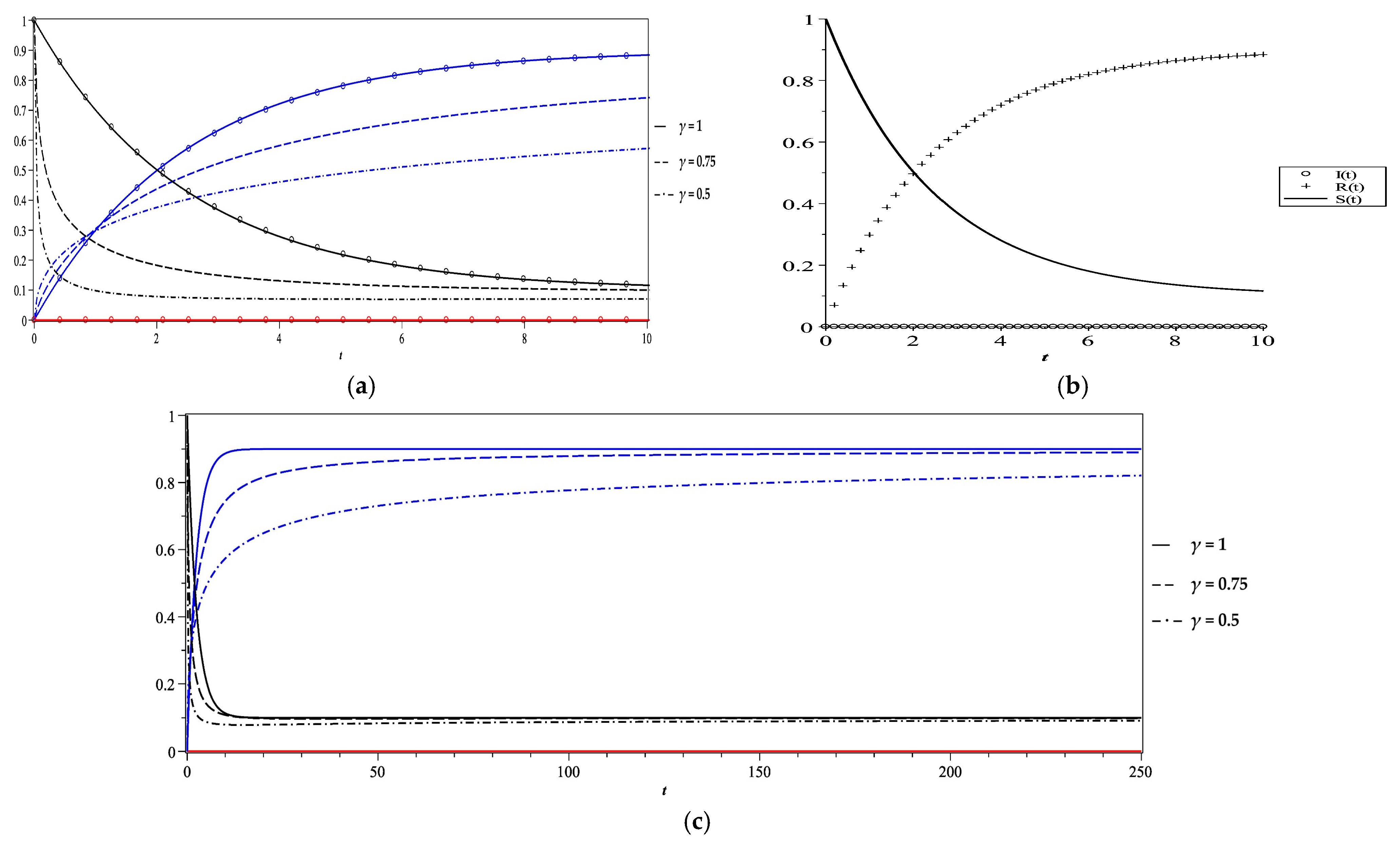
1	0.186	1	0.1	0.0	0.9	0.1000	0.0	0.8999	Removal of the disease
		0.75				0.0989	0.0	0.8897
		0.5				0.0914	0.0	0.8207
2	0.186	1	0.1	0.0	0.9	0.0999	0.0	0.9000
		0.75				0.0989	0.0	0.8897
		0.5				0.0913	0.0	0.8208
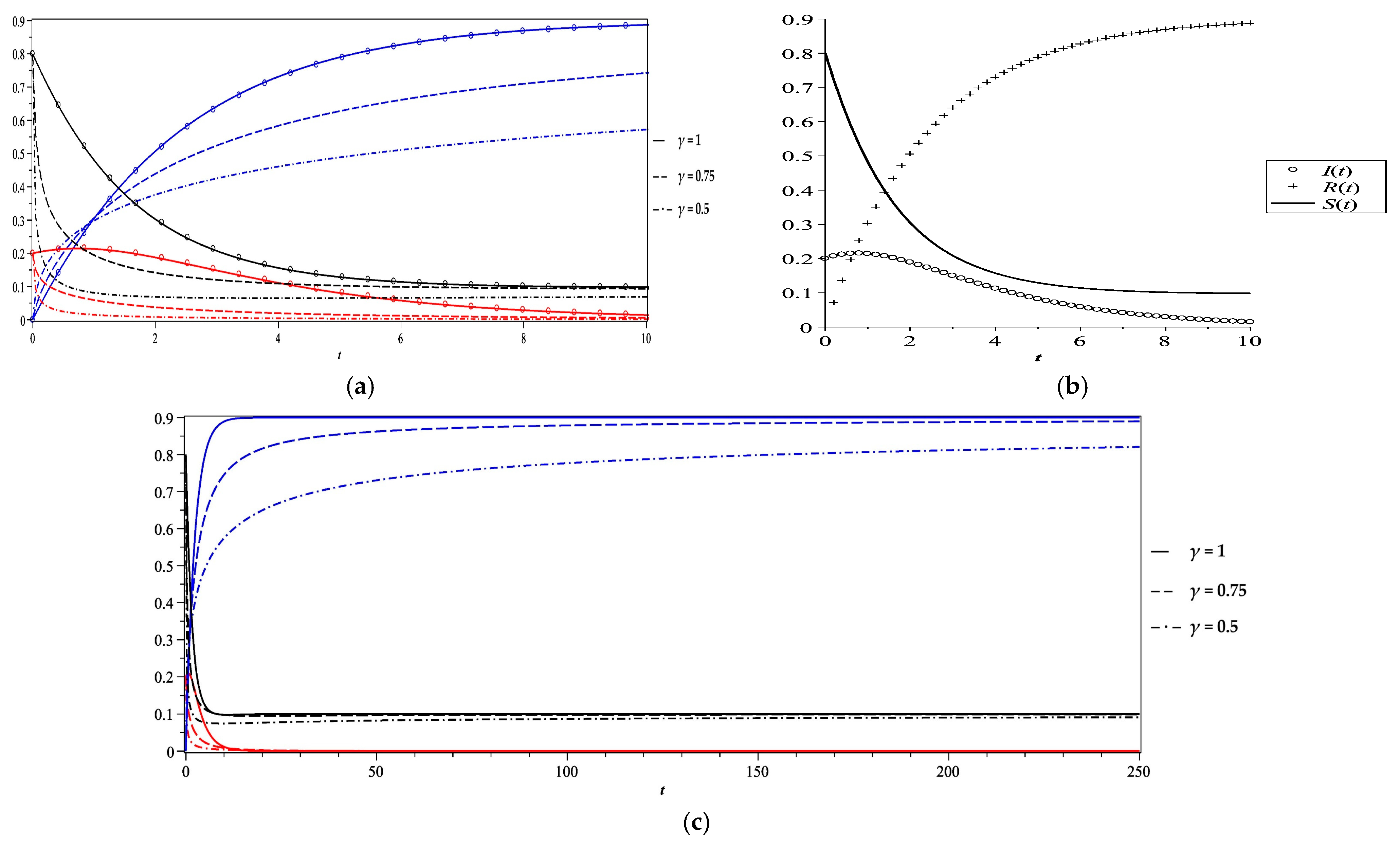
3	1.302	1	0.5375	0.1512	0.3113	0.5375	0.1512	0.3113	No removal of the disease
		0.75				0.5457	0.1363	0.3066
		0.5				0.6277	0.0102	0.2742
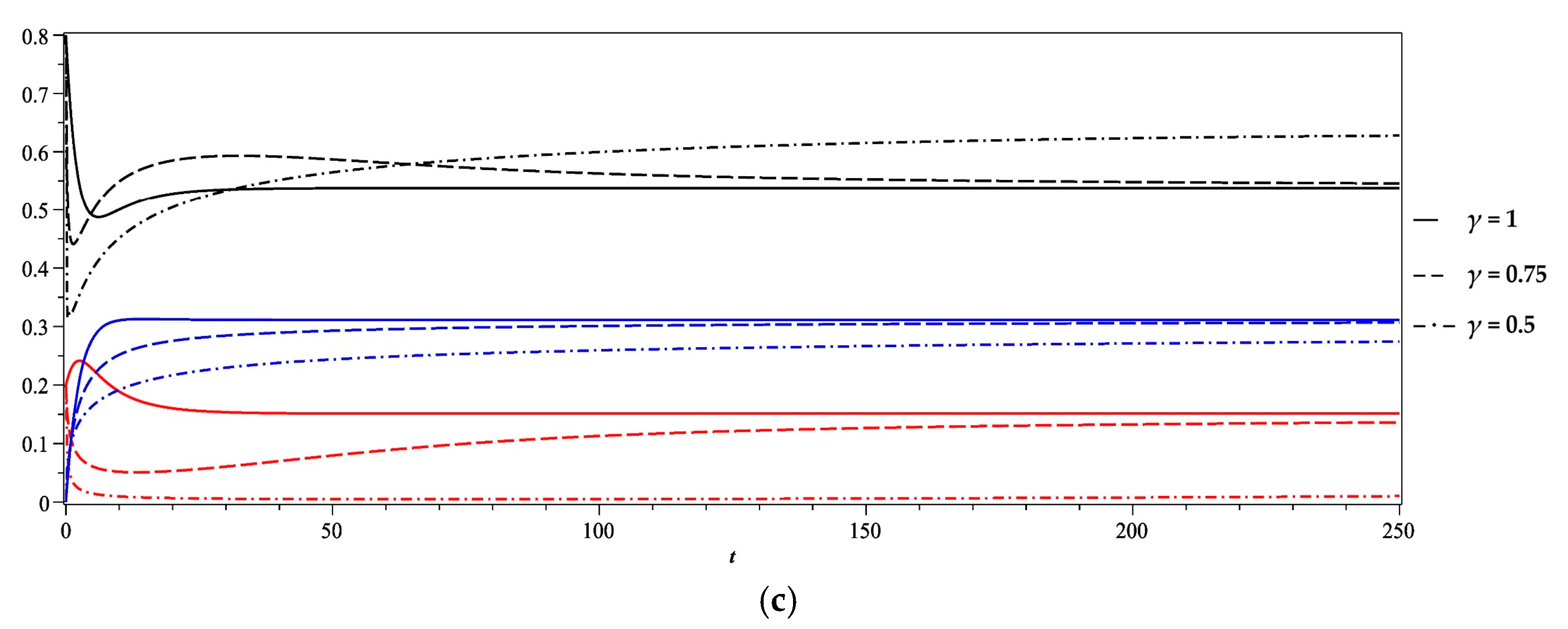
4	1.860	1	0.5375	0.4302	0.0323	0.5375	0.4302	0.0323
		0.75				0.5440	0.4140	0.0306
		0.5				0.6063	0.2870	0.0188

which illustrates how the model dynamics differently behave as per parameters values changed. From the data presented in the table, it is clear that the numerical results are in excellent agreement with the results of the system fixed points in both disease-free equilibrium and endemic equilibrium case. For the disease-free equilibrium cases, the fraction of the infected population is vanishing for all values of the fractional order γ by the time and hence a disease has been eradicated. While for the endemic equilibrium cases, the fraction of the infected population decreases with the decreasing of the fractional order γ by the time, but the disease is not eradicated.

6. Conclusions

This paper deals with a new application of a Grünwald–Letnikov method for the achievement of a numerical simulation of a fractional-order SIR epidemiological diseases model. The significant advantage of the considered technique is that it can be used without system linearization or any other restrictions for any fractional-order dynamical system. A stability analysis is performed to qualitatively investigate the dynamics of the model in both disease-free and endemic equilibrium case. It is explained that the graphical representation presented in [1,2] are inaccurate. One of the issues that validates the present results is the excellent agreement between them with the results presented in [3] and RK4 results for integer order γ = 1. The excellent agreement between the asymptotic behavior of the solutions with the numerical results is another evident on the validation and the reliability of the considered numerical technique in studying such dynamical models in epidemiology. The proposed technique is reliable and accurate in simulating the behavior of the solutions for a long-time interval. The disease-free equilibrium is stable if the vaccination amount above a critical value p_c. The dynamics of the model is strongly dependent on the value of the fractional order γ. For the endemic equilibrium cases, the fraction of the infected population decreases by the reduction of the fractional order γ as time passes.

References

- Ullah, A.; Abdeljawad, T.; Ahmad, S.; Shah, K.; Karapinar, E. Study of a fractional-order epidemic model of childhood diseases. J. Funct. Spaces 2020, 2020, 5895310. [Google Scholar] [CrossRef] [PubMed]
- Haq, F.; Shahzad, M.; Muhammad, S.; Wahab, H.A.; Rahman, G.U. Numerical analysis of fractional order epidemic model of childhood diseases. Discret. Dyn. Nat. Soc. 2017, 2017, 4057089. [Google Scholar] [CrossRef]
- Makinde, O.D. Adomian decomposition approach to a SIR epidemic model with constant vaccination strategy. Appl. Math. Comput. 2007, 184, 842–848. [Google Scholar] [CrossRef]
- Rachah, A.; Torres, D.F.M. Mathematical modelling, simulation, and optimal control of the 2014 ebola outbreak in West Africa. Discret. Dyn. Nat. Soc. 2015, 2015, 842792. [Google Scholar]
- GA, N.; MI, T.-E. A Mathematical model with quarantine states for the dynamics of Ebola virus disease in human populations. Comput. Math. Methods Med. 2016, 2016, 9352725. [Google Scholar]
- Ogunlaran, O.M.; Noutchie, S.C. Mathematical model for an effective management of HIV infection. Biomed. Res. Int. 2016, 2016, 4217548. [Google Scholar] [CrossRef]
- Djordjevic, J.; Silva, C.J.; Torres, D.F.M. A stochastic SICA epidemic model for HIV transmission. Appl. Math. Lett. 2018, 84, 168–175. [Google Scholar] [CrossRef] [Green Version]
- Arenas, A.J.; González-Parra, G.; Naranjo, J.J.; Cogollo, M.; La Espriella, N.D. Mathematical analysis and numerical solution of a model of HIV with a discrete time delay. Mathematics 2021, 9, 257. [Google Scholar] [CrossRef]
- Zafar, Z.U.A.; Rehan, K.; Mushtaq, M. HIV/AIDS epidemic fractional-order model. J. Differ. Equ. Appl. 2017, 23, 1298–1315. [Google Scholar] [CrossRef]
- Omame, A.; Abbas, M.; Onyenegecha, C.P. A fractional-order model for COVID-19 and tuberculosis co-infection using Atangana–Baleanu derivative. Chaos Solitons Fractals 2021, 153, 111486. [Google Scholar] [CrossRef] [PubMed]
- Okuonghae, D.; Omame, A. Analysis of a mathematical model for COVID-19 population dynamics in Lagos, Nigeria. Chaos Solitons Fractals 2020, 139, 110032. [Google Scholar] [CrossRef]
- Cooper, I.; Mondal, A.; Antonopoulos, C.G. A SIR model assumption for the spread of COVID-19 in different communities. Chaos Solitons Fractals 2020, 139, 110057. [Google Scholar] [CrossRef] [PubMed]
- Singh, H.; Srivastava, H.M.; Hammouch, Z.; Nisar, K.S. Numerical simulation and stability analysis for the fractional-order dynamics of COVID-19. Results Phys. 2021, 20, 103722. [Google Scholar] [CrossRef] [PubMed]
- Yadav, S.; Kumar, D.; Singh, J.; Baleanu, D. Analysis and dynamics of fractional order Covid-19 model with memory effect. Results Phys. 2021, 24, 104017. [Google Scholar] [CrossRef]
- Moreno, V.M.; Espinoza, B.; Bichara, D.; Holechek, S.A.; Castillo-Chavez, C. Role of short-term dispersal on the dynamics of Zika virus in an extreme idealized environment. Infect. Dis. Model. 2017, 2, 21–34. [Google Scholar] [CrossRef]
- Ndaïrou, F.; Area, I.; Nieto, J.J.; Silva, C.J.; Torres, D.F.M. Mathematical modeling of Zika disease in pregnant women and newborns with microcephaly in Brazil. Math. Methods Appl. Sci. 2018, 41, 8929–8941. [Google Scholar] [CrossRef] [Green Version]
- Ndaïrou, F.; Area, I.; Torres, D.F.M. Mathematical modeling of Japanese encephalitis under aquatic environmental effects. Mathematics 2020, 8, 1880. [Google Scholar] [CrossRef]
- Angstmann, C.N.; Henry, B.I.; McGann, A.V. A fractional order recovery SIR model from a stochastic process. Bull. Math. Biol. 2016, 78, 468–499. [Google Scholar] [CrossRef] [Green Version]
- Al-Sulami, H.; El-Shahed, M.; Nieto, J.J.; Shammakh, W. On fractional order dengue epidemic model. Math. Probl. Eng. 2014, 2014, 456537. [Google Scholar] [CrossRef]
- Sweilam, N.H.; AL-Mekhlafi, S.M.; Baleanu, D. Optimal control for a fractional tuberculosis infection model including the impact of diabetes and resistant strains. J. Adv. Res. 2019, 17, 125–137. [Google Scholar] [CrossRef]
- Ndaïrou, F.; Area, I.; Nieto, J.J.; Silva, C.J.; Torres, D.F.M. Fractional model of COVID-19 applied to Galicia, Spain and Portugal. Chaos Solitons Fractals 2021, 144, 110652. [Google Scholar] [CrossRef]
- Du, M.; Wang, Z.; Hu, H. Measuring memory with the order of fractional derivative. Sci. Rep. 2013, 3, 3431. [Google Scholar] [CrossRef] [PubMed]
- Lichae, B.H.; Biazar, J.; Ayati, Z. The fractional differential model of HIV-1 infection of CD4+ T-Cells with description of the effect of antiviral drug treatment, Comput. Math. Methods Med. 2019, 2019, 4059549. [Google Scholar] [CrossRef] [Green Version]
- Danane, J.; Allali, K.; Hammouch, Z. Mathematical analysis of a fractional differential model of HBV infection with antibody immune response. Chaos Solitons Fractals 2020, 136, 109787. [Google Scholar] [CrossRef]
- Li, Y.; Haq, F.; Shah, K.; Shahzad, M.; Rahman, G. Numerical analysis of fractional order Pine wilt disease model with bilinear incident rate. J. Math. Comput. Sci. 2017, 17, 420–428. [Google Scholar] [CrossRef] [Green Version]
- Owolabi, K.M.; Atangana, A. Mathematical modelling and analysis of fractional epidemic models using derivative with exponential kernel. In Fractional Calculus in Medical and Health Science; CRC Press: Boca Raton, FL, USA, 2020; pp. 109–128. [Google Scholar]
- El-Dessoky, M.M.; Khan, M.A. Modeling and analysis of an epidemic model with fractal-fractional Atangana-Baleanu derivative. Alex. Eng. J. 2022, 61, 729–746. [Google Scholar] [CrossRef]
- Dorcak, L. Numerical models for the simulation of the fractional-order control systems. arXiv 2002, arXiv:math/0204108v1. [Google Scholar]
- Vinagre, B.M.; Chen, Y.Q.; Petráš, I. Two direct Tustin discretization methods for fractional-order differentiator/integrator. J. Frankl. Inst. 2003, 340, 349–362. [Google Scholar] [CrossRef]
- Podlubny, I. Fractional Differential Equations: An Introduction to Fractional Derivatives, Fractional Differential Equations, to Methods of Their Solution and Some of Their Applications; Academic Press: New York, NY, USA, 1998. [Google Scholar]
- Petráš, I. Fractional-Order Nonlinear Systems: Modeling, Analysis and Simulation; Springer: Berlin, Germany, 2011. [Google Scholar]
- Tavazoei, M.S.; Haeri, M. A necessary condition for double scroll attractor existence in fractional-order systems. Phys. Lett. A 2007, 367, 102–113. [Google Scholar] [CrossRef]