Reachable Set and Robust Mixed Performance of Uncertain Discrete Systems with Interval Time-Varying Delay and Linear Fractional Perturbations

Abstract

In this paper, the mixed performance and reachable set of uncertain discrete systems with slow variation interval time-varying delay are considered. The original uncertain discrete systems with interval time-varying delay are first transformed into a switched system. Then, the proposed improved results are used to guarantee the stability and reachable set of the uncertain system with slow variation interval time-varying delay. The mixed performance (H₂/H_∞) can be derived in the same formulation simultaneously. The design scheme of robust switched control is also developed in this paper. The gains of the controller can be designed and switched to achieve stabilization and mixed performance of the system according to the delay value. Some comparisons with published results are made to show the main contribution of the proposed approach. Finally, some numerical examples are illustrated to show the main results.

1. Introduction

Time delay is confronted in many practical systems, such as chemical engineering systems, hydraulic systems, inferred grinding models, neural networks, population dynamic models, and rolling mills. Instability or bad performance may cause the appearance of time delay in many control systems [1,2,3]. It is also interesting to note that interval time-varying delay is a more suitable type that describes the physical environment for signal transmission [4,5,6,7]. Hence, we consider herein the uncertain discrete system with interval time-varying delay.

In recent years, many performance issues of switched systems have been considered. The dynamics of switched systems comprise a family of subsystems and use a switching signal to handle the switching between the subsystems. Switched systems are encountered in many practical models, such as automotive engine control, chemical processes, constrained robotics, multi-rate control, power systems and power electronics, robot manufacture, stepper motors, and water quality control [8,9]. It is also well known that many complicated nonlinear dynamical system behaviors, such as multiple limit cycles and chaos, may be caused by switching among subsystems [8,9]. Hence, the stability and performance of switched systems have been investigated in recent years [10,11,12,13,14,15]. It is also interesting to note that the stability of a switched system can be guaranteed by selecting an appropriate switching signal, even when each subsystem is unstable [13,14]. Hence, switching control can be designed by using the switching signal.

The reachable set of a control system is used to show the set containing all states of the system reachable from the origin for a bounded peak disturbance [4,6,10,12,16,17,18]. In [4], the reachable set of systems of a switched system was investigated by a multiple Lyapunov strategy. In [9], the dwell time approach was applied to estimate the reachable set of the switched system under consideration. In [6], the reachable set of a discrete system with interval time-varying delay was estimated by the Lyapunov method. In [12], the switched system approach in [4] was applied to estimate the reachable set of the system under consideration in [6]. The switched system approach in [4] was illustrated to be less conservative by the proposed numerical examples.

The $H_{\infty }$ performance of systems has been used in recent years to inspect the effect of regulated output with respect to disturbance input and guarantee that the closed-loop system is stable [19,20,21]. The $H_2$ performance of systems is another requirement that has been applied to minimize a quadratic performance index about the initial state of a system under no disturbance input [22]. Hence, the $H_2$/$H_{\infty }$ mixed performance has been an interesting research topic in recent years [23,24,25]. In this paper, the reachable set and mixed $H_2$/$H_{\infty }$ performance are considered. Minimization of the $H_{\infty }$ performance with the $H_2$ norm constraint is developed. Moreover, it is well known that linear fractional perturbation is a more general representation than norm bounded uncertainties of the systems under consideration [13,19,21,25,26,27]. To the best of the authors’ knowledge, there are few results considering the reachable set and mixed performance of an uncertain discrete system with interval time-varying delay and linear fractional perturbations. In this paper, the LMI optimization approach in [28] is used to minimize $H_{\infty }$ performance under some $H_2$ norm constraints. The main contributions of this paper can be highlighted as follows:

(1)

Reachable set estimation and mixed $H_2$ /$H_{\infty }$ performance for an uncertain discrete system with interval time-varying delay and linear fractional perturbations are considered in this paper.

(2)

A new improved analytic result is proposed based on the approach developed in [4]. Less conservative results for an uncertain discrete system with slow variation interval time-varying delay are provided for more accurate estimation of the reachable set. The $H_2$ /$H_{\infty }$ performance can also be guaranteed from the design scheme.

(3)

The LMI optimization approach is used to guarantee the minimization of the reachable set and achievement of mixed performance of the system under consideration. The proposed conditions can be solved easily by the Matlab LMI toolbox.

The remainder of this paper is organized as follows. The problem formulation is given in Section 2. The main results are given in Section 3. Section 4 provides some numerical examples to illustrate the main results. Finally, conclusions are drawn in Section 5.

Notation: For a matrix A, we denote the transpose by $A^T$ and symmetric positive (negative) definite by $A>0$ ($A<0$). $A\le B$ means that matrix $B-A$ is symmetric positive semi-definite. $Sym\left(X\right)=X+X^T$, and $I$ and 0 denote the identity matrix and zero matrix with appropriate dimensions, respectively; $0_{l\times m}$ and $I_n$ denote the zero matrix with dimensions $l\times m$ and identity matrix with dimensions $n\times n$, respectively. Diag [$\begin{array}{ccc}{A}_1& \cdots & A_r\end{array}$] denotes the block diagonal matrix with matrices $\begin{array}{ccc}{A}_1& \cdots & A_r\end{array}$ on its diagonal, $E_{qi}=\left[\begin{array}{ccc}{0}_{n\times \left(i-1\right)n}& I_n& 0_{n\times \left(q-i\right)n}\end{array}\right]\in {\Re }^{n\times qn}$, $i=1,\hspace{0.33em}2,\hspace{0.33em}\cdots ,\hspace{0.33em}q$, $q=2,\hspace{0.33em}3,\cdots ,7$, $A\backslash B=\left\{x\left|x\in A\hspace{0.33em}and\hspace{0.33em}x\notin B\right.\right\}$, $S\left(r\right)=\left\{s\in {\Re }^n\left|s^{T}s<r\right.,r>0\right\}$, $L_2\left(0,\infty \right)=\left\{w\in {\Re }^l\left|{\displaystyle \sum }_{k=0}^{k=\infty }{w}^T\left(k\right)w\left(k\right)<\infty \right.\right\}$, $\underset{\_}{N}=\left\{1,\hspace{0.33em}2,\hspace{0.33em}\cdots ,\hspace{0.33em}N\right\}$, and $\Vert x\Vert$ denotes the Euclidean norm of vector x.

2. Problem Formulation and Mixed Performance Analysis

Consider the following uncertain discrete system with interval time-varying delay:

$$x\left(k+1\right)={\stackrel{-}{A}}_0\left(k\right)x\left(k\right)+{\stackrel{-}{A}}_1\left(k\right)x\left(k-\tau \left(k\right)\right)+{\stackrel{-}{B}}_{xw}\left(k\right)w\left(k\right),\hspace{0.33em}k\ge 0$$

(1a)

$$z\left(k\right)={\stackrel{-}{A}}_{z0}\left(k\right)x\left(k\right)+{\stackrel{-}{A}}_{z1}\left(k\right)x\left(k-\tau \left(k\right)\right)+{\stackrel{-}{B}}_{zw}\left(k\right)w\left(k\right),k\ge 0$$

(1b)

$$x\left(\theta \right)=\varphi \left(\theta \right),\theta =-{\tau }_M,\hspace{0.33em}-{\tau }_M+1,\hspace{0.33em}\cdots ,\hspace{0.33em}0$$

(1c)

where $x\left(k\right)\in {\Re }^n$ is the state; $w\left(k\right)\in {\Re }^m$ is the disturbance input; $z\left(k\right)\in {\Re }^l$ is the regulated output; $\varphi$ is the initial function; $\tau \left(k\right)$ is the interval time-varying delay satisfying ${\tau }_m\le \tau \left(k\right)\le {\tau }_M$; ${\tau }_m$ and ${\tau }_M$ are two given positive integers; perturbed matrices ${\stackrel{-}{A}}_i\left(k\right)=A_i+\mathsf{\Delta }{A}_i\left(k\right)$, ${\stackrel{-}{A}}_{zi}\left(k\right)=A_{zi}+\mathsf{\Delta }{A}_{zi}\left(k\right)$, $i=0,\hspace{0.33em}1$, ${\stackrel{-}{B}}_{xw}\left(k\right)=B_{xw}+\mathsf{\Delta }{B}_{xw}\left(k\right)$, ${\stackrel{-}{B}}_{zw}\left(k\right)=B_{zw}+\mathsf{\Delta }{B}_{zw}\left(k\right)$, $A_i$, $A_{zi}$, $B_{xw}$, and $B_{zw}$ are constant matrices with appropriate dimensions; and $\mathsf{\Delta }{A}_i\left(k\right)$, $\mathsf{\Delta }{A}_{zi}\left(k\right)$, $\mathsf{\Delta }{B}_{xw}\left(k\right)$, and $\mathsf{\Delta }{B}_{zw}\left(k\right)$ are some perturbed matrices that satisfy the following linear fractional perturbation conditions:

$$\left[\begin{array}{ccc}\mathsf{\Delta }{A}_0\left(k\right)& \mathsf{\Delta }{A}_1\left(k\right)& \mathsf{\Delta }{B}_{xw}\left(k\right)\end{array}\right]=M_x\cdot {\mathsf{\Delta }}_1\left(k\right)\cdot \left[\begin{array}{ccc}{N}_0& N_1& N_{2w}\end{array}\right],\hspace{0.33em}\forall \hspace{0.33em}k\ge 0,$$

(2a)

$$\left[\begin{array}{ccc}\mathsf{\Delta }{A}_{z0}\left(k\right)& \mathsf{\Delta }{A}_{z1}\left(k\right)& \mathsf{\Delta }{B}_{zw}\left(k\right)\end{array}\right]=M_z\cdot {\mathsf{\Delta }}_2\left(k\right)\cdot \left[\begin{array}{ccc}{N}_3& N_4& N_{5w}\end{array}\right],\hspace{0.33em}\forall \hspace{0.33em}k\ge 0,$$

(2b)

$${\mathsf{\Delta }}_j\left(k\right)={\left[I-{\Gamma }_j\left(k\right){\Xi }_j\right]}^{-1}{\Gamma }_j\left(k\right),{\Xi }_j{\Xi }_j^T<I,j=1,\hspace{0.33em}2$$

(2c)

where $M_x\in {\Re }^{n\times n}$, $M_z\in {\Re }^{l\times l}$, ${\Xi }_j$, $j=1,\hspace{0.33em}2$, $N_l$, $l=0,\hspace{0.33em}1,3,4$, and $N_{kw}$, $k=2,\hspace{0.33em}5$ are some given constant matrices with appropriate dimensions. ${\Gamma }_j\left(k\right)$, $j=1,\hspace{0.33em}2$, are unknown matrices representing the parameter perturbations which satisfy

$${\Gamma }_j{(k)}^T\cdot {\Gamma }_j\left(k\right)\le I,j=1,\hspace{0.33em}2,k\ge 0.$$

Now, we consider the interval time-varying delay $\tau \left(k\right)$ satisfying the following condition:

$$\left|\tau \left(k+1\right)-\tau \left(k\right)\right|\le \lambda ,$$

(3)

where $\lambda$ is a non-negative integer with $1<{\tau }_m\le \tau \left(k\right)\le {\tau }_M$. If $\lambda =1$, we have the following three possible conditions: $\tau \left(k+1\right)=\tau \left(k\right)$, $\tau \left(k+1\right)=\tau \left(k\right)+1$, and $\tau \left(k+1\right)=\tau \left(k\right)-1$. By using the switching approach, the original system (1) can be rewritten as

$$x\left(k+1\right)={\stackrel{-}{A}}_0\left(k\right)x\left(k\right)+{\stackrel{-}{A}}_1\left(k\right)x\left(k-{\tau }_{\sigma \left(k\right)}\left(k\right)\right)+{\stackrel{-}{B}}_{xw}\left(k\right)w\left(k\right),\hspace{0.33em}k\ge 0,$$

(4a)

$$z\left(k\right)={\stackrel{-}{A}}_{z0}\left(k\right)x\left(k\right)+{\stackrel{-}{A}}_{z1}\left(k\right)x\left(k-{\tau }_{\sigma \left(k\right)}\left(k\right)\right)+{\stackrel{-}{B}}_{zw}\left(k\right)w\left(k\right),k\ge 0,$$

(4b)

$$x\left(\theta \right)=\varphi \left(\theta \right),\theta =-{\tau }_M,\hspace{0.33em}-{\tau }_M+1,\hspace{0.33em}\cdots ,\hspace{0.33em}0,$$

(4c)

where switching signal $\sigma \left(k\right)=\tau \left(k\right)-\left({\tau }_m-1\right)\in \underset{\_}{N}$, $N={\tau }_M-{\tau }_m+1$, and ${\tau }_{\sigma \left(k\right)}\left(k\right)=\tau \left(k\right)$. With respect to $\tau \left(k\right)={\tau }_m$ and $\tau \left(k\right)={\tau }_M$, we have $\sigma \left(k\right)=1$ and $\sigma \left(k\right)=N$, respectively. With the constraint in (3), we have

$$\left|\sigma \left(k+1\right)-\sigma \left(k\right)\right|\le \lambda .$$

(5)

We define

$$X\left(k\right)={\left[x^T\left(k\right)x^T\left(k-1\right)x^T\left(k-2\right)\cdots x^T\left(k-{\tau }_M\right)\right]}^T.$$

We then have

$$X\left(k+1\right)=[{\overline{A}}_{X0}\left(k\right)+{\overline{A}}_{X1}\left(k\right)E_{\sigma \left(k\right)}]X\left(k\right)+{\overline{B}}_{Xw}\left(k\right)w\left(k\right),\hspace{0.33em}k\ge 0,$$

(6a)

$$z\left(k\right)=[{\overline{A}}_{Z0}\left(k\right)+{\overline{A}}_{Z1}\left(k\right)E_{\sigma \left(k\right)}]X\left(k\right)+{\overline{B}}_{Zw}\left(k\right)w\left(k\right),\hspace{0.33em}k\ge 0,$$

(6b)

$$X\left(0\right)=\overline{\varphi },$$

(6c)

where $\overline{\varphi }=\left[{\varphi }^T\left(0\right){\varphi }^T\left(-1\right){\varphi }^T\left(-2\right)\cdots {\varphi }^T\left(-{\tau }_M\right)\right]$,

$${\overline{A}}_{X0}\left(k\right)=\left[\begin{array}{ccccc}{\stackrel{-}{A}}_0\left(k\right)& 0& \cdots & 0& 0\\ I& 0& 0& 0& 0\\ 0& I& 0& 0& 0\\ ⋮& ⋮& \ddots & 0& 0\\ 0& 0& \cdots & I& 0\end{array}\right]=A_{X0}+\left[\begin{array}{c}{M}_x\\ 0_{n·{\tau }_M\times n}\end{array}\right]\cdot {\mathsf{\Delta }}_1\left(k\right)\cdot \left[\begin{array}{cc}{N}_0& 0_{n\times n·{\tau }_M}\end{array}\right],$$

$${\overline{A}}_{X1}\left(k\right)=\left[\begin{array}{c}{\stackrel{-}{A}}_1\left(k\right)\\ 0\\ \begin{array}{c}0\\ \begin{array}{c}⋮\\ 0\end{array}\end{array}\end{array}\right]=\left[\begin{array}{c}{\stackrel{-}{A}}_1\left(k\right)\\ 0_{n·{\tau }_M\times n}\end{array}\right]=A_{X1}+\left[\begin{array}{c}{M}_x\\ 0_{n·{\tau }_M\times n}\end{array}\right]\cdot {\mathsf{\Delta }}_1\left(k\right)\cdot N_1,$$

$${\stackrel{-}{B}}_{Xw}\left(k\right)=\left[\begin{array}{c}{\stackrel{-}{B}}_w\left(k\right)\\ 0\\ \begin{array}{c}0\\ \begin{array}{c}⋮\\ 0\end{array}\end{array}\end{array}\right]=\left[\begin{array}{c}{\stackrel{-}{B}}_{xw}\left(k\right)\\ 0_{n·{\tau }_M\times m}\end{array}\right]=B_{Xw}+\left[\begin{array}{c}{M}_x\\ 0_{n·{\tau }_M\times n}\end{array}\right]\cdot {\mathsf{\Delta }}_1\left(k\right)\cdot N_{2w},$$

$$A_{X0}=\left[\begin{array}{ccccc}{A}_0& 0& \cdots & 0& 0\\ I& 0& 0& 0& 0\\ 0& I& 0& 0& 0\\ ⋮& ⋮& \ddots & 0& 0\\ 0& 0& \cdots & I& 0\end{array}\right],A_{X1}=\left[\begin{array}{c}{A}_1\\ 0_{n·{\tau }_M\times n}\end{array}\right],B_{Xw}=\left[\begin{array}{c}{B}_{xw}\\ 0_{n·{\tau }_M\times m}\end{array}\right],$$

$$E_{\sigma \left(k\right)}=\left[\begin{array}{ccc}\begin{array}{cc}{0}_{n\times n·{\tau }_m}& 0_{n\times n·\left(\sigma \left(k\right)-1\right)}\end{array}& I& 0_{n\times n·\left(N-\sigma \left(k\right)\right)}\end{array}\right]$$

$${\stackrel{-}{A}}_{Z0}\left(k\right)=\left[\begin{array}{ccc}{\stackrel{-}{A}}_{z0}\left(k\right)& 0& \begin{array}{cc}\cdots & 0\end{array}\end{array}\right]=\left[\begin{array}{cc}{\stackrel{-}{A}}_{z0}\left(k\right)& 0_{l\times n·{\tau }_M}\end{array}\right]$$

$$=\left[\begin{array}{cc}{A}_{z0}& 0_{l\times n·{\tau }_M}\end{array}\right]+M_z\cdot {\mathsf{\Delta }}_2\left(k\right)\cdot \left[\begin{array}{cc}{N}_3& 0_{l\times n·{\tau }_M}\end{array}\right],$$

$${\stackrel{-}{A}}_{Z1}\left(k\right)={\stackrel{-}{A}}_{z1}\left(k\right)=A_{z1}+M_z\cdot {\mathsf{\Delta }}_2\left(k\right)\cdot N_4,{\stackrel{-}{B}}_{Zw}\left(k\right)={\stackrel{-}{B}}_{zw}\left(k\right)=B_{zw}+M_z\cdot {\mathsf{\Delta }}_2\left(k\right)\cdot N_{5w},$$

$$A_{Z0}=\left[\begin{array}{cc}{A}_{z0}& 0_{l\times n·{\tau }_M}\end{array}\right],A_{Z1}=A_{z1},B_{Zw}=B_{zw}.$$

With the consideration for the reachable set, we may assume bounded peak disturbance satisfying

$$w^T\left(k\right)w\left(k\right)\le {\stackrel{-}{w}}^2,\forall k\ge 0,$$

(7)

where $\stackrel{-}{w}>0$ is a given constant. We give the following definition.

Definition 1 ([25]).

Consider the system (1) with (2) and (7). Assume the following:

(i)

With $w\left(k\right)=0$, the system (1) with (2) and (7) is asymptotically stable, and we can find an $\alpha >0$ to satsify the inequality

$${{\displaystyle \sum }}_{k=0}^{k={\mathcal{\ell }}_1}{z}^T\left(k\right)z\left(k\right)\le \alpha ,$$

for any positive integer${\mathcal{\ell }}_1$.

(ii)

With zero initial conditions (i.e., $\varphi \left(k\right)=0,\hspace{0.33em}-{\tau }_M\le k\le 0$,the signals $w\left(k\right)$ and $z\left(k\right)$ are bounded by

$${{\displaystyle \sum }}_{k=0}^{k={\mathcal{\ell }}_2}{z}^T\left(k\right)z\left(k\right)\le {\gamma }^2\cdot {{\displaystyle \sum }}_{k=0}^{k={\mathcal{\ell }}_2}{w}^T\left(k\right)w\left(k\right),\forall \hspace{0.33em}w\ne 0,$$

for any positive integer${\mathcal{\ell }}_2$and constant$\gamma$.

If the parameter ${\mathcal{\ell }}_2$ is selected as $\infty$, the disturbance input $w$ should be constrained in $L_2\left(0,\infty \right)$. Then we say that the system (1) with (2) and (7) is asymptotically stable with $H_2$ measure $\alpha$ and $H_{\infty }$ performance $\gamma$. If the disturbance is constrained in (7) for a given $\overline{w}>0$, we can find a set $R$ where $x\left(k\right)\in R$, $\forall \hspace{0.33em}k>0$. This set $R\subseteq {\Re }^n$ is called the reachable set of the system.

The following lemmas will be used to derive the main results in this paper.

Lemma 1

([28]).(Schur complement) For a given matrix $S=\left[\begin{array}{cc}{S}_{11}& S_{12}\\ *& S_{22}\end{array}\right]$ with $S_{11}=S_{11}^T$ and $S_{22}=S_{22}^T$, the following conditions are equivalent:

$$\left(1\right) S<0;$$

$$\left(2\right) S_{22}<0, S_{11}-S_{12}{S}_{22}^{-1}{S}_{12}^T<0.$$

Lemma 2

([26,27]). Suppose that ${\mathsf{\Delta }}_1\left(t\right)$ is defined in (2a) and satisfies (2c); then, for real matrices $U$, $W$, and $X$ with $X=X_{}^T$, the following statements are equivalent:

(I)

The following inequality is satisfied:

$$X+U{\mathsf{\Delta }}_1\left(t\right)W+W_{}^T{\mathsf{\Delta }}_1^T\left(t\right)U_{}^T<0;$$

(II)

There exists a scalar $\epsilon >0$ such that

$$\left[\begin{array}{ccc}X& U& \epsilon \cdot W_{}^T\\ *& -\epsilon \cdot I& \epsilon \cdot {\Xi }_1^T\\ *& *& -\epsilon \cdot I\end{array}\right]<0$$

or

$$\left[\begin{array}{ccc}X& \epsilon \cdot U& W_{}^T\\ *& -\epsilon \cdot I& \epsilon \cdot {\Xi }_1^T\\ *& *& -\epsilon \cdot I\end{array}\right]<0,$$

where the matrix ${\Xi }_1$ is as defined in (2c).

Lemma 3 ([12]).

Consider a switched system in (6) with bounded peak disturbance in (7). Let $V_i\left(X\left(k\right)\right)$, $i\in \underset{-}{N}$ be a Lyapunov function satisfying $V_i\left(0\right)=0$ and $V_i\left(X\left(k\right)\right)>0$, $\forall X\left(k\right)\ne 0$, $i\in \underset{-}{N}$. If there exist constants $0<{\alpha }_{ji}<1$, $i,j\in \underset{-}{N}$, such that

$$V_j\left(X\left(k+1\right)\right)-{\alpha }_{ji}·V_i\left(X\left(k\right)\right)-\frac{1-{\alpha }_{ji}}{{\overline{w}}^2}{w}^T\left(k\right)w\left(k\right)<0,\forall i,j\in \underset{-}{N},$$

(8a)

then the system is asymptotically stable and we have

$$V_i\left(X\left(k\right)\right)\le 1,i\in \underset{-}{N},\mathit{for}\mathit{all}{V}_i\left(X\left(0\right)\right)\le 1,i\in \underset{-}{N}.$$

Proof. 

With $w\left(k\right)=0$, we have the following result from (8a):

$$V_i\left(X\left(k+1\right)\right)-V_i\left(X\left(k\right)\right)\le V_i\left(X\left(k+1\right)\right)-{\alpha }_{ji}·V_i\left(X\left(k\right)\right)<0.$$

This implies that the system is asymptotically stable. With the bounded peak disturbance in (7) and $V_i\left(X\left(k\right)\right)\le 1$, we have

$$V_j\left(X\left(k+1\right)\right)-{\alpha }_{ji}·V_i\left(X\left(k\right)\right)<\frac{1-{\alpha }_{ji}}{{\overline{w}}^2}{w}^T\left(k\right)w\left(k\right)\le 1-{\alpha }_{ji}.$$

This implies

$$V_j\left(X\left(k+1\right)\right)-1\le {\alpha }_{ji}·(V_i\left(X\left(k\right)\right)-1.$$

With $\sigma \left(k+1\right)=j$ and $\sigma \left(k\right)=i$, we have

$$V_{\sigma \left(k+1\right)}\left(X\left(k+1\right)\right)-1\le {\alpha }_{\sigma \left(k+1\right)\sigma \left(k\right)}·\left(V_{\sigma \left(k\right)}\left(X\left(k\right)\right)-1\right)$$

$$\le {\alpha }_{\sigma \left(k+1\right)\sigma \left(k\right)}·{\alpha }_{\sigma \left(k\right)\sigma \left(k-1\right)}·\left(V_{\sigma \left(k-1\right)}\left(X\left(k-1\right)\right)-1\right)$$

$$\le {\alpha }_{\sigma \left(k+1\right)\sigma \left(k\right)}·{\alpha }_{\sigma \left(k\right)\sigma \left(k-1\right)}\cdots ·{\alpha }_{\sigma \left(1\right)\sigma \left(0\right)}\left(V_{\sigma \left(0\right)}\left(X\left(0\right)\right)-1\right).$$

When $V_{\sigma \left(0\right)}\left(X\left(0\right)\right)\le 1$, we have

$$V_i\left(X\left(k\right)\right)\le 1,i\in \underset{-}{N}.\square$$

Lemma 4 ([12]).

Consider a switched system in (6) with bounded peak disturbance in (7). If there exist matrices$P_i\in {\Re }^{n·({\tau }_M+1)\times n·({\tau }_M+1)}$, $i\in \underset{-}{N}$, and constants${\delta }_i$, $0<{\alpha }_{ji}<1$, $i,j\in \underset{-}{N}$, such that

$$\left[\begin{array}{cc}{[{\overline{A}}_{X0}\left(k\right)+{\overline{A}}_{X1}\left(k\right)E_i]}^T{P}_j[{\overline{A}}_{X0}\left(k\right)+{\overline{A}}_{X1}\left(k\right)E_i]-{\alpha }_{ji}{P}_i& {[{\overline{A}}_{X0}\left(k\right)+{\overline{A}}_{X1}\left(k\right)E_i]}^T{P}_j{\stackrel{-}{B}}_{Xw}\left(k\right)\\ *& {\stackrel{-}{B}}_{Xw}^T\left(k\right)P_j{\stackrel{-}{B}}_{Xw}\left(k\right)-\frac{1-{\alpha }_{ji}}{{\overline{w}}^2}·I\end{array}\right]<0,\forall i,j\in \underset{-}{N},$$

(8b)

$$\left[\begin{array}{cccc}I& 0& \cdots & 0\\ 0& 0& \cdots & 0\\ ⋮& ⋮& \ddots & ⋮\\ 0& 0& \cdots & 0\end{array}\right]<{\delta }_i{P}_i,\forall i\in \stackrel{-}{N},$$

then the system is asymptotically stable and the reachable set is bounded by a hyper-sphere$S\left(r\right)$ with $r=\underset{i\in \underset{-}{N}}{\min }{\delta }_i$.

For the above proposed condition in (8b), it is difficult to solve and decompose the system with uncertainties; we developed the following results to find the feasible solution.

Lemma 5.

Consider a switched system in (6) with bounded peak disturbance in (7). If there exist matrices$P_i\in {\Re }^{n·({\tau }_M+1)\times n·({\tau }_M+1)}$, $i\in \underset{-}{N}$, and constants${\delta }_i$, $0<{\alpha }_{ji}<1$, $i,j\in \underset{-}{N}$, such that

$$\left[\begin{array}{ccc}-{\alpha }_{ji}·P_i& 0& {\left({\overline{A}}_{X0}\left(k\right)+{\overline{A}}_{X1}\left(k\right)E_i\right)}^T{P}_j\\ *& -\frac{1-{\alpha }_{ji}}{{\overline{w}}^2}·I& {\stackrel{-}{B}}_{Xw}{\left(k\right)}^T{P}_j\\ *& *& -P_j\end{array}\right]<0,\forall i,j\in \underset{-}{N},$$

(9)

$$\left[\begin{array}{cccc}I& 0& \cdots & 0\\ 0& 0& \cdots & 0\\ ⋮& ⋮& \ddots & ⋮\\ 0& 0& \cdots & 0\end{array}\right]<{\delta }_i{P}_i,\forall i\in \underset{-}{N},$$

then the system is asymptotically stable and the reachable set is bounded by a hyper-sphere$S\left(r\right)$with$r=\underset{i\in \underset{-}{N}}{\min }{\delta }_i$.

Proof. 

Define the following Lyapunov function:

$$V_{\sigma \left(k\right)}\left(X\left(k\right)\right)=X{\left(k\right)}^T{P}_{\sigma \left(k\right)}X\left(k\right).$$

With $\sigma \left(k\right)=i$, $\sigma \left(k+1\right)=j$, we have

$$\begin{gathered} V_j\left(X\left(k+1\right)\right)-{\alpha }_{ji}·V_i\left(X\left(k\right)\right)-\frac{1-{\alpha }_{ji}}{{\overline{w}}^2}{w}^T\left(k\right)w\left(k\right) \\ =X{\left(k+1\right)}^T{P}_{j}X\left(k+1\right)-{\alpha }_{ji}·X{\left(k\right)}^T{P}_{i}X\left(k\right)-\frac{1-{\alpha }_{ji}}{{\overline{w}}^2}{w}^T\left(k\right)w\left(k\right). \end{gathered}$$

(10a)

We define

$$\overline{X}\left(k\right)={\left[\begin{array}{cc}{X}^T\left(k\right)& w^T\left(k\right)\end{array}\right]}^T,$$

$$X\left(k+1\right)=\left[\begin{array}{cc}{\overline{A}}_{X0}\left(k\right)+{\overline{A}}_{X1}\left(k\right)E_i& {\stackrel{-}{B}}_{Xw}\left(k\right)\end{array}\right]\overline{X}\left(k\right).$$

We have the following result from (9):

$$V_j\left(X\left(k+1\right)\right)-{\alpha }_{ji}·V_i\left(X\left(k\right)\right)-\frac{1-{\alpha }_{ji}}{{\overline{w}}^2}{w}^T\left(k\right)w\left(k\right)={\overline{X}}^T\left(k\right){\mathsf{\Delta }}_i\left(k\right)\overline{X}{\left(k\right)}^T,$$

where

$$\begin{gathered} {\mathsf{\Delta }}_i\left(k\right)=\left[\begin{array}{cc}-{\alpha }_{ji}·P_i& 0\\ 0& -\frac{1-{\alpha }_{ji}}{{\overline{w}}^2}·I\end{array}\right] \\ +\left[\begin{array}{c}{\left({\overline{A}}_{X0}\left(k\right)+{\overline{A}}_{X1}\left(k\right)E_i\right)}^T\\ {\stackrel{-}{B}}_{Xw}{\left(k\right)}^T\end{array}\right]P_j\left[\begin{array}{cc}{\overline{A}}_{X0}\left(k\right)+{\overline{A}}_{X1}\left(k\right)E_i& {\stackrel{-}{B}}_{Xw}\left(k\right)\end{array}\right]. \end{gathered}$$

(10b)

By the Schur complement in Lemma 1, the conditions in (9) imply $\mathsf{\Delta }\left(k\right)<0$ in (10b). This proof can be completed in view of Lemmas 3 and 4. □

Remark 1.

Lemmas 4 and 5 can be applied to guarantee the asymptotic stability and reachable set of system (1) with (2) and (7). However, the proposed condition in (9) can be used to solve the system under consideration with perturbations and obtain LMI conditions that are easy to solve without uncertain elements by the LMI toolbox of Matlab.

3. Main Results

From (6), the condition in (9) is equivalent to

$$\begin{gathered} \left[\begin{array}{ccc}-{\alpha }_{ji}·P_i& 0& {\left({\stackrel{-}{A}}_{X0}\left(k\right)+{\stackrel{-}{A}}_{X1}\left(k\right)E_i\right)}^T{P}_j\\ *& -\frac{1-{\alpha }_{ji}}{{\stackrel{-}{w}}^2}·I& {\stackrel{-}{B}}_{Xw}{\left(k\right)}^T{P}_j\\ *& *& -P_j\end{array}\right] \\ =\left[\begin{array}{ccc}-{\alpha }_{ji}·P_i& 0& {\left(A_{X0}+A_{X1}{E}_i\right)}^T{P}_j\\ *& -\frac{1-{\alpha }_{ji}}{{\stackrel{-}{w}}^2}·I& B_{Xw}{}^T{P}_j\\ *& *& -P_j\end{array}\right]+Sym(\left[\begin{array}{c}{0}_{n·\left({\tau }_M+1\right)\times n}\\ 0_{m\times n}\\ P_j\left[\begin{array}{c}{M}_x\\ 0_{n·{\tau }_M\times n}\end{array}\right]\end{array}\right]·{\mathsf{\Delta }}_x\left(k\right)·{\stackrel{=}{N}}_i)<0 \end{gathered}$$

(11a)

where

$${\stackrel{=}{N}}_i=\left[\left(\left[\begin{array}{cc}{N}_0& 0_{n\times n·{\mathsf{\tau }}_M}\end{array}\right]+N_1{E}_i\right)N_{2w}{0}_{n\times (n·{\mathsf{\tau }}_M+1)}\right].$$

By using Lemma 2, the condition in (11a) is equivalent to

$$\left[\begin{array}{ccccc}-{\alpha }_{ji}·P_i& 0& {\left(A_{X0}+A_{X1}{E}_i\right)}^T{P}_j& 0_{n·\left({\tau }_M+1\right)\times n}& {\aleph }_{15ij}\\ *& -\frac{1-{\alpha }_{ji}}{{\stackrel{-}{w}}^2}·I& B_{Xw}{}^T{P}_j& 0_{m\times n}& {\epsilon }_{ij}·N_{2w}^T\\ *& *& -P_j& P_j\left[\begin{array}{c}{M}_x\\ 0_{n·{\tau }_M\times n}\end{array}\right]& 0_{n·\left({\tau }_M+1\right)\times n}\\ *& *& *& -{\epsilon }_{ij}·I& {\epsilon }_{ij}·{\Xi }_1^T\\ *& *& *& *& -{\epsilon }_{ij}·I\end{array}\right]<0,$$

(11b)

where ${\aleph }_{15ij}={\epsilon }_{ij}·{\left(\left[\begin{array}{cc}{N}_0& 0_{n\times n·{\tau }_M}\end{array}\right]+N_1{E}_i\right)}^T$.

The following LMI result is proposed to guarantee the mixed performance and reachable set of system (1) with (2) and (7).

Theorem 1.

If there exist constants ${\delta }_i$, $0<{\alpha }_{ji}<1$, $i,j\in \underset{-}{N}$, such that the LMI conditions

$$\left[\begin{array}{ccccc}-{\alpha }_{ji}·P_i& 0& {\left(A_{X0}+A_{X1}{E}_i\right)}^T{P}_j& 0_{n·\left({\tau }_M+1\right)\times n}& {\aleph }_{15ij}\\ *& -\frac{1-{\alpha }_{ji}}{{\stackrel{-}{w}}^2}·I& B_{Xw}{}^T{P}_j& 0_{m\times n}& {\epsilon }_{ij}·N_{2w}^T\\ *& *& -P_j& P_j\left[\begin{array}{c}{M}_x\\ 0_{n·{\tau }_M\times n}\end{array}\right]& 0_{n·\left({\tau }_M+1\right)\times n}\\ *& *& *& -{\epsilon }_{ij}·I& {\epsilon }_{ij}·{\Xi }_1^T\\ *& *& *& *& -{\epsilon }_{ij}·I\\ & & i,j\in \underset{-}{N},& & \end{array}\right]<0,$$

(12a)

$$\left[\begin{array}{cccc}I& 0& \cdots & 0\\ 0& 0& \cdots & 0\\ ⋮& ⋮& \ddots & ⋮\\ 0& 0& \cdots & 0\end{array}\right]<{\delta }_i{P}_i,\hspace{1em}i\in \underset{-}{N},$$

(12b)

$${\mathsf{\Omega }}_i=\left[\begin{array}{cccccccc}-P& 0& {\mathsf{\Omega }}_{i13}& {\mathsf{\Omega }}_{i14}& 0_{n·\left({\tau }_M+1\right)\times n}& {\mathsf{\Omega }}_{i16}& 0_{n·\left({\tau }_M+1\right)\times l}& {\mathsf{\Omega }}_{i18}\\ *& -\overline{\gamma }·I& {B_{XW}}^{T}P& {B_{Zw}}^T& 0_{m\times n}& {\mathsf{\Omega }}_{i26}& 0_{m\times l}& {\mathsf{\Omega }}_{i28}\\ *& *& -P& 0& {\mathsf{\Omega }}_{i35}& 0_{n·\left({\tau }_M+1\right)\times n}& 0_{n·\left({\tau }_M+1\right)\times l}& 0_{n·\left({\tau }_M+1\right)\times l}\\ *& *& *& -I& 0_{l\times n}& 0_{l\times n}& M_z& 0_{l\times l}\\ *& *& *& *& -{\eta }_{xi}·I& {\eta }_{xi}·{\Xi }_1^T& 0& 0\\ *& *& *& *& *& -{\eta }_{xi}·I& 0& 0\\ *& *& *& *& *& *& -{\eta }_{zi}·I& {\eta }_{zi}·{\Xi }_2^T\\ *& *& *& *& *& *& *& -{\eta }_{zi}·I\end{array}\right],i\in \underset{-}{N},$$

(12c)

$$\left[\begin{array}{cc}-\alpha & {\overline{\varphi }}^{T}P\\ P\overline{\varphi }& -P\end{array}\right]<0,$$

(12d)

where$\overline{\gamma }={\gamma }^2$,

$${\aleph }_{15ij}={\epsilon }_{ij}·{\left(\left[\begin{array}{cc}{N}_0& 0_{n\times n·{\tau }_M}\end{array}\right]+N_1{E}_i\right)}^T$$

$$\begin{gathered} {\mathsf{\Omega }}_{i13}={[A_{X0}+A_{X1}{E}_i]}^{T}P,{\mathsf{\Omega }}_{i14}={[A_{Z0}+A_{Z1}{E}_i]}^T,{\mathsf{\Omega }}_{i16}={\eta }_{xi}·{\left(\left[\begin{array}{cc}{N}_0& 0_{n\times n·{\tau }_M}\end{array}\right]+N_1{E}_i\right)}^T, \\ {\mathsf{\Omega }}_{i18}={\eta }_{zi}·{\left(\left[\begin{array}{cc}{N}_3& 0_{l\times n·{\tau }_M}\end{array}\right]+N_4{E}_i\right)}^T,{\mathsf{\Omega }}_{i26}={\eta }_{xi}·N_{2w}{}^T,{\mathsf{\Omega }}_{i28}={\eta }_{zi}·N_{5w}{}^T, \end{gathered}$$

$${\mathsf{\Omega }}_{i35}=P\left[\begin{array}{c}{M}_x\\ 0_{n·{\tau }_M\times n}\end{array}\right],$$

have a feasible solution with some positive definite symmetric matrices$P$, $P_i\in {\Re }^{n·({\tau }_M+1)\times n·({\tau }_M+1)}$, $i\in \underset{-}{N}$, and positive constants$\alpha$, $\overline{\gamma }$, ${\delta }_i$,${\eta }_{xi}$and${\eta }_{zi}$, and${\epsilon }_{ij}$, $i,j\in \underset{-}{N}$, then the system (1) with (2) is asymptotically stable with$H_2$asure$\alpha$and$H_{\infty }$performance$\gamma =\sqrt{\overline{\gamma }}$, and the reachable set is bounded by a hyper-sphere$S\left(a\right)$with$a=\underset{i\in \underset{-}{N}}{\min }{\delta }_i$.

Proof. 

The first part of the proof about stability and the reachable set can be completed using Lemma 5 and derivations in (11). Now we wish to solve the uncertain system with mixed $H_2$/$H_{\infty }$ performance. We define the following Lyapunov function:

$$V\left(X\left(k\right)\right)=X^T\left(k\right)PX\left(k\right),$$

(13)

where $P\in {\Re }^{n·({\tau }_M+1)\times n·({\tau }_M+1)}$. We define $Y\left(k\right)={\left[X^T\left(k\right)w^T\left(k\right)\right]}^T$, and from the difference of Lyapunov function (13) along the solutions of system (6), we have

$$\begin{gathered} z^T\left(k\right)z\left(k\right)-{\gamma }^2·w^T\left(k\right)w\left(k\right)+\mathsf{\Delta }V\left(X\left(k\right)\right) \\ =z^T\left(k\right)z\left(k\right)-{\gamma }^2·w^T\left(k\right)w\left(k\right)+X^T\left(k+1\right)PX\left(k+1\right)-X^T\left(k\right)PX\left(k\right) \\ =Y^T\left(k\right){\mathsf{\Psi }}_{\sigma \left(k\right)}\left(k\right)Y\left(k\right), \end{gathered}$$

(14a)

where

$$\begin{gathered} {\mathsf{\Psi }}_{\sigma \left(k\right)}\left(k\right)=\left[\begin{array}{cc}-P& 0\\ 0& -{\gamma }^2·I\end{array}\right]+\left[\begin{array}{c}{[{\overline{A}}_{X0}\left(k\right)+{\overline{A}}_{X1}\left(k\right)E_{\sigma \left(k\right)}]}^T\\ {\overline{B}}_{Xw}{\left(k\right)}^T\end{array}\right]P{\left[\begin{array}{c}{[{\overline{A}}_{X0}\left(k\right)+{\overline{A}}_{X1}\left(k\right)E_{\sigma \left(k\right)}]}^T\\ {\overline{B}}_{Xw}{\left(k\right)}^T\end{array}\right]}^T \\ +\left[\begin{array}{c}{[{\overline{A}}_{Z0}\left(k\right)+{\overline{A}}_{Z1}\left(k\right)E_{\sigma \left(k\right)}]}^T\\ {\overline{B}}_{Zw}{\left(k\right)}^T\end{array}\right]{\left[\begin{array}{c}{[{\overline{A}}_{Z0}\left(k\right)+{\overline{A}}_{Z1}\left(k\right)E_{\sigma \left(k\right)}]}^T\\ {\overline{B}}_{Zw}{\left(k\right)}^T\end{array}\right]}^T. \end{gathered}$$

We define

$$\begin{gathered} {\mathsf{\Lambda }}_{\sigma \left(k\right)}\left(k\right)=\left[\begin{array}{cccc}-P& 0& {[{\overline{A}}_{X0}\left(k\right)+{\overline{A}}_{X1}\left(k\right)E_{\sigma \left(k\right)}]}^{T}P& {[{\overline{A}}_{Z0}\left(k\right)+{\overline{A}}_{Z1}\left(k\right)E_{\sigma \left(k\right)}]}^T\\ *& -{\gamma }^2·I& {\overline{B}}_{Xw}{\left(k\right)}^{T}P& {\overline{B}}_{Zw}{\left(k\right)}^T\\ *& *& -P& 0\\ *& *& *& -I\end{array}\right] \\ =\left[\begin{array}{cccc}-P& 0& {[A_{X0}+A_{X1}{E}_{\sigma \left(k\right)}]}^{T}P& {[A_{Z0}+A_{Z1}{E}_{\sigma \left(k\right)}]}^T\\ *& -{\gamma }^2·I& B_{Xw}{}^{T}P& B_{Zw}{}^T\\ *& *& -P& 0\\ *& *& *& -I\end{array}\right] \\ +Sym\left(\left[\begin{array}{c}{0}_{n·\left({\tau }_M+1\right)\times n}\\ 0_{m\times n}\\ P\left[\begin{array}{c}{M}_x\\ 0_{n·{\tau }_M\times n}\end{array}\right]\\ 0_{l\times n}\end{array}\right]\cdot {\mathsf{\Delta }}_x\left(k\right)\cdot {\stackrel{=}{N}}_x\right)+Sym\left(\left[\begin{array}{c}{0}_{n·\left({\tau }_M+1\right)\times l}\\ 0_{m\times l}\\ 0_{n·\left({\tau }_M+1\right)\times l}\\ M_z\end{array}\right]\cdot {\mathsf{\Delta }}_z\left(k\right)\cdot {\stackrel{=}{N}}_z\right), \end{gathered}$$

(14b)

where

$$\begin{gathered} {\stackrel{=}{N}}_x=\left[\left(\left[\begin{array}{cc}{N}_0& 0_{n\times n·{\tau }_M}\end{array}\right]+N_1{E}_{\sigma \left(k\right)}\right)N_{2w}{0}_{n\times n·\left({\tau }_M+1\right)}{0}_{n\times l}\right], \\ {\stackrel{=}{N}}_z=\left[\left(\left[\begin{array}{cc}{N}_3& 0_{l\times n·{\tau }_M}\end{array}\right]+N_4{E}_{\sigma \left(k\right)}\right)N_{5w}{0}_{l\times n·\left({\tau }_M+1\right)}{0}_{l\times l}\right]. \end{gathered}$$

Assume $\sigma \left(k\right)=i\in \underset{-}{N}$, and from (14b) and Lemma 2, we can define ${\mathsf{\Omega }}_i$ in (12c). By using Lemma 2, the condition ${\mathsf{\Omega }}_i<0$ in (12c) implies ${\mathsf{\Lambda }}_i\left(k\right)<0$ in (14b). From Lemma 1, the condition ${\mathsf{\Lambda }}_i\left(k\right)<0$ in (14b) also imples ${\mathsf{\Psi }}_i\left(k\right)<0$ in (14a). From ${\mathsf{\Psi }}_i\left(k\right)<0$ in (14a), we have

$$z^T\left(k\right)z\left(k\right)-{\gamma }^2·w^T\left(k\right)w\left(k\right)+\mathsf{\Delta }V\left(X\left(k\right)\right)<0,\forall Y\left(k\right)\ne 0.$$

(15)

Summing the equation (8a) from 0 to ${\mathcal{\ell }}_2$, we have

$$V\left(X\left(k\right)\right)-V\left(X\left(0\right)\right)+{{\displaystyle \sum }}_{k=0}^{{\mathcal{\ell }}_2}\left[z^T\left(k\right)z\left(k\right)-{\gamma }^2\cdot w^T\left(k\right)w\left(k\right)\right]\le 0.$$

With zero initial condition ($X\left(0\right)=0,\varphi \left(k\right)=0,\hspace{0.33em}-{\tau }_M\le k\le 0$), we have

$$V\left(X\left(0\right)\right)=0.$$

By the definition of Lyapunov function $V\left(X\left(k\right)\right)$ in (13), we have

$$V\left(X\left(k\right)\right)\ge 0.$$

(16)

From the above derivations, the following condition can be guaranteed:

$${{\displaystyle \sum }}_{k=0}^{{\mathcal{\ell }}_2}{z}^T\left(k\right)z\left(k\right)\le {\gamma }^2\cdot {{\displaystyle \sum }}_{k=0}^{{\mathcal{\ell }}_2}{w}^T\left(k\right)w\left(k\right),\forall \hspace{0.33em}w\ne 0.$$

By using (12d) with Lemma 1, we have

$${\overline{\varphi }}^T\left(0\right)P\overline{\varphi }<\alpha .$$

With $w\left(k\right)=0$, (12d), and (15), (16), we have

$${{\displaystyle \sum }}_{k=0}^{{\mathcal{\ell }}_1}{z}^T\left(k\right)z\left(k\right)\le V\left(\overline{\varphi }\right)={\overline{\varphi }}^T\left(0\right)P\overline{\varphi }<\alpha .$$

This completes the proof. □

For simplicity, we can obtain the following optimization result by $\delta ={\delta }_i$ and ${\alpha }_0={\alpha }_{ij}$, $\forall i,j\in \underset{-}{N}$.

Corollary 1.

Suppose there exists a constant$0<{\alpha }_0<1$, such that the optimization problem

$$\underset{i=1,2,3,4}{\mathrm{minimize}}\hspace{1em}{\delta }_i>0\mathrm{or}\overline{\gamma }>0\mathrm{or}\alpha >0,$$

subject to

$$\left[\begin{array}{ccccc}-{\alpha }_0·P_i& 0& {\left(A_{X0}+A_{X1}{E}_i\right)}^T{P}_j& 0_{n·\left({\tau }_M+1\right)\times n}& {\aleph }_{15ij}\\ *& -\frac{1-{\alpha }_0}{{\overline{w}}^2}·I& B_{Xw}{}^T{P}_j& 0_{m\times n}& {\epsilon }_{ij}·N_{2w}^T\\ *& *& -P_j& P_j\left[\begin{array}{c}{M}_x\\ 0_{n·{\tau }_M\times n}\end{array}\right]& 0_{n·\left({\tau }_M+1\right)\times n}\\ *& *& *& -{\epsilon }_{ij}·I& {\epsilon }_{ij}·{\Xi }_1^T\\ *& *& *& *& -{\epsilon }_{ij}·I\end{array}\right]<0,i,j\in \underset{-}{N},$$

(17a)

$$\left[\begin{array}{cccc}I& 0& \cdots & 0\\ 0& 0& \cdots & 0\\ ⋮& ⋮& \ddots & ⋮\\ 0& 0& \cdots & 0\end{array}\right]<{\delta }_i{P}_i,i\in \underset{-}{N},$$

(17b)

$${\mathsf{\Omega }}_i=\left[\begin{array}{cccccccc}-P& 0& {\mathsf{\Omega }}_{i13}& {\mathsf{\Omega }}_{i14}& 0_{n·\left({\tau }_M+1\right)\times n}& {\mathsf{\Omega }}_{i16}& 0_{n·\left({\tau }_M+1\right)\times l}& {\mathsf{\Omega }}_{i18}\\ *& -\overline{\gamma }·I& {B_X}^{T}P& {B_{Zw}}^T& 0_{m\times n}& {\mathsf{\Omega }}_{i26}& 0_{m\times l}& {\mathsf{\Omega }}_{i28}\\ *& *& -P& 0& {\mathsf{\Omega }}_{i35}& 0_{n·\left({\tau }_M+1\right)\times n}& 0_{n·\left({\tau }_M+1\right)\times l}& 0_{n·\left({\tau }_M+1\right)\times l}\\ *& *& *& -I& 0_{l\times n}& 0_{l\times n}& M_z& 0_{l\times l}\\ *& *& *& *& -{\eta }_{xi}·I& {\eta }_{xi}·{\Xi }_1^T& 0& 0\\ *& *& *& *& *& -{\eta }_{xi}·I& 0& 0\\ *& *& *& *& *& *& -{\eta }_{zi}·I& {\eta }_{zi}·{\Xi }_2^T\\ *& *& *& *& *& *& *& -{\eta }_{zi}·I\end{array}\right],i\in \underset{-}{N},$$

(17c)

$$\left[\begin{array}{cc}-\alpha & {\overline{\varphi }}^{T}P\\ P\overline{\varphi }& -P\end{array}\right]<0,$$

(17d)

where$\overline{\gamma }={\gamma }^2$,

$$\begin{gathered} {\aleph }_{15ij}={\epsilon }_{ij}·{\left(\left[\begin{array}{cc}{N}_0& 0_{n\times n·{\tau }_M}\end{array}\right]+N_1{E}_i\right)}^T, \\ {\mathsf{\Omega }}_{i13}={[A_{X0}+A_{X1}{E}_i]}^{T}P,{\mathsf{\Omega }}_{i14}={[A_{Z0}+A_{Z1}{E}_i]}^T,{\mathsf{\Omega }}_{i16}={\eta }_{xi}·{\left(\left[\begin{array}{cc}{N}_0& 0_{n\times n·{\tau }_M}\end{array}\right]+N_1{E}_i\right)}^T, \\ {\mathsf{\Omega }}_{i18}={\eta }_{zi}·{\left(\left[\begin{array}{cc}{N}_3& 0_{l\times n·{\tau }_M}\end{array}\right]+N_4{E}_i\right)}^T \\ ,{\mathsf{\Omega }}_{i26}={\eta }_{xi}·N_{2w}{}^T,{\mathsf{\Omega }}_{i28}={\eta }_{zi}·N_{5w}{}^T, \\ {\mathsf{\Omega }}_{i35}=P\left[\begin{array}{c}{M}_x\\ 0_{n·{\tau }_M\times n}\end{array}\right], \end{gathered}$$

has a feasible solution with some positive definite symmetric matrices$P$, $P_i\in {\Re }^{n·({\tau }_M+1)\times n·({\tau }_M+1)}$, $i\in \underset{-}{N}$, and positive constants$\alpha$, $\overline{\gamma }$, ${\eta }_{xi}$, ${\eta }_{zi}$, and${\epsilon }_{ij}$, $i,j\in \underset{-}{N}$. Then, the system (1) with (2) is asymptotically stable with$H_2$measure$\alpha$and$H_{\infty }$performance$\gamma =\sqrt{\overline{\gamma }}$, and the reachable set is bounded by a hyper-sphere$S\left(a\right)$with$a=\underset{i\in N}{\mathit{min}}{\delta }_i$.

Remark 2.

Under the variation constraint in (3) and (5), the constant $\lambda \ge 0$ represents the variation in the delay and switching signal with $N={\tau }_M-{\tau }_m+1$. If the value is small (for example, $\lambda =1$ or $\lambda =2$), we can say that it is a discrete system with slow variation in time-varying delay. When $\lambda =1$, for the LMI condition terms in (8b), (9), (12a), and (17a), we can use $i\in \underset{-}{N}$, $j=i-1,i,i+1\in \underset{-}{N}$ instead of $i,j\in \underset{-}{N}$. When $\lambda =2$, for the LMI condition terms in (8b), (9), (12a), and (17a), we can use $i\in \underset{-}{N}$, $j=i-2,i-1,i,i+1,i+2\in \underset{-}{N}$ instead of $i,j\in \underset{-}{N}$. Hence, the proposed results for a system under a slow variation constraint on time-varying delay will be less conservative than those without this constraint.

Remark 3.

In Theorem 1 and Corollary 1, we can take minimization about$\overline{\gamma }={\gamma }^2$ or $\alpha$ with respect to the LMI conditions in (12). The optimal $H_2$ measure or $H_{\infty }$ performance of the system can be finished using the Matlab toolbox from our proposed results. Smaller values of $\gamma$ and $\alpha$ will imply better disturbance attenuation and $H_2$ measure, respectively. The minimization of $\delta$ can be used to give a more exact evaluation of the reachable set. Now we provide a procedure around the results of Corollary 1 to ensure the stability and reachable set for the system under consideration. With the selection of ${\alpha }_0$, the optimization in (17) of Corollary 1 can be formulated as follows:

Step 1. Set ${\delta }_1=\cdots ={\delta }_{j-1}={\delta }_{j+1}=\cdots ={\delta }_N=1000$ (or a larger constant) and perform minimization on ${\delta }_j$; the optimization in (17) has a feasible solution.

Step 2. Minimize the value $\overline{\gamma }$ with a feasible solution for optimization in (17).

Step 3. The value $\alpha$ can be minimized for a feasible solution of optimization in (17) at this final step.

Consider the following uncertain discrete system with interval time-varying delay and control input:

$$x\left(k+1\right)={\stackrel{-}{A}}_0\left(k\right)x\left(k\right)+{\stackrel{-}{A}}_1\left(k\right)x\left(k-\tau \left(k\right)\right)+{\stackrel{-}{B}}_{xw}\left(k\right)w\left(k\right)+{\stackrel{-}{B}}_{xu}\left(k\right)u\left(k\right),\hspace{0.33em}k\ge 0,$$

(18a)

$$z\left(k\right)={\stackrel{-}{A}}_{z0}\left(k\right)x\left(k\right)+{\stackrel{-}{A}}_{z1}\left(k\right)x\left(k-\tau \left(k\right)\right)+{\stackrel{-}{B}}_{zw}\left(k\right)w\left(k\right)+{\stackrel{-}{B}}_{zu}\left(k\right)u\left(k\right),k\ge 0,$$

(18b)

$$x\left(\theta \right)=\varphi \left(\theta \right),\theta =-{\tau }_M,\hspace{0.33em}-{\tau }_M+1,\hspace{0.33em}\cdots ,\hspace{0.33em}0,$$

(18c)

where $x\left(k\right)\in {\Re }^n$ is the state; $w\left(k\right)\in {\Re }^m$ is the disturbance input; $z\left(k\right)\in {\Re }^l$ is the regulated ouput; $u\left(k\right)\in {\Re }^p$ is the control input; $\varphi$ is the initial function $;\tau \left(k\right)$ is the interval time-varying delay satisfying ${\tau }_m\le \tau \left(k\right)\le {\tau }_M$; ${\tau }_m$ and ${\tau }_M$ are two positive integers; perturbed matrices ${\stackrel{-}{A}}_i\left(k\right)=A_i+\mathsf{\Delta }{A}_i\left(k\right)$, ${\stackrel{-}{A}}_{zi}\left(k\right)=A_{zi}+\mathsf{\Delta }{A}_{zi}\left(k\right)$, ${\stackrel{-}{B}}_{xw}\left(k\right)=B_{xw}+\mathsf{\Delta }{B}_{xw}\left(k\right)$, ${\stackrel{-}{B}}_{xu}\left(k\right)=B_{xu}+\mathsf{\Delta }{B}_{xu}\left(k\right)$, ${\stackrel{-}{B}}_{zw}\left(k\right)=B_{zw}+\mathsf{\Delta }{B}_{zw}\left(k\right)$, ${\stackrel{-}{B}}_{zu}\left(k\right)=B_{zu}+\mathsf{\Delta }{B}_{zu}\left(k\right)$, $i=0,\hspace{0.33em}1$, $A_i$, $A_{zi}$, $B_{xw}$, $B_{xu}$, $B_{zw}$, and $B_{zu}$ are constant matrices with appropriate dimensions; and $\mathsf{\Delta }{A}_i\left(k\right)$, $\mathsf{\Delta }{A}_{zi}\left(k\right)$, $\mathsf{\Delta }{B}_{xw}\left(k\right)$,$\mathsf{\Delta }{B}_{xu}\left(k\right)$, $\mathsf{\Delta }{B}_{zw}\left(k\right)$, and $\mathsf{\Delta }{B}_{zu}\left(k\right)$ are some perturbed matrices that satisfy the following linear fractional perturbation conditions:

$$\left[\begin{array}{cccc}\mathsf{\Delta }{A}_0\left(k\right)& \mathsf{\Delta }{A}_1\left(k\right)& \mathsf{\Delta }{B}_{xw}\left(k\right)& \mathsf{\Delta }{B}_{xu}\left(k\right)\end{array}\right]=M_x\cdot {\mathsf{\Delta }}_1\left(k\right)\cdot \left[\begin{array}{cccc}{N}_0& N_1& N_{2w}& N_{2u}\end{array}\right],$$

(19a)

$$\left[\begin{array}{cccc}\mathsf{\Delta }{A}_{z0}\left(k\right)& \mathsf{\Delta }{A}_{z1}\left(k\right)& \mathsf{\Delta }{B}_{zw}\left(k\right)& \mathsf{\Delta }{B}_{zu}\left(k\right)\end{array}\right]=M_z\cdot {\mathsf{\Delta }}_2\left(k\right)\cdot \left[\begin{array}{cccc}{N}_3& N_4& N_{5w}& N_{5u}\end{array}\right],$$

(19b)

$${\mathsf{\Delta }}_j\left(k\right)={\left[I-{\Gamma }_j\left(k\right){\Xi }_j\right]}^{-1}{\Gamma }_j\left(k\right),{\Xi }_j{\Xi }_j^T<I,j=1,\hspace{0.33em}2,$$

(19c)

where $M_x\in {\Re }^{n\times n}$, $M_z\in {\Re }^{l\times l}$, ${\Xi }_j$, $j=1,\hspace{0.33em}2$, $N_l$, $l=0,\hspace{0.33em}1,3,4$, $N_{2w}$, $N_{2u}$, $N_{5w}$, and $N_{5u}$, are some given constant matrices with appropriate dimensions. ${\Gamma }_j\left(k\right)$, $j=1,\hspace{0.33em}2$, are unknown matrices representing the parameter perturbations which satisfy

$${\Gamma }_j{(k)}^T\cdot {\Gamma }_j\left(k\right)\le I,j=1,\hspace{0.33em}2,k\ge 0.$$

By using the switching approach, the original system (1) can be rewritten as:

$$x\left(k+1\right)={\stackrel{-}{A}}_0\left(k\right)x\left(k\right)+{\stackrel{-}{A}}_1\left(k\right)x\left(k-{\tau }_{\sigma \left(k\right)}\left(k\right)\right)+{\stackrel{-}{B}}_{wx}\left(k\right)w\left(k\right)+{\stackrel{-}{B}}_{xu}\left(k\right)u\left(k\right),\hspace{0.33em}k\ge 0,$$

(20a)

$$z\left(k\right)={\stackrel{-}{A}}_{z0}\left(k\right)x\left(k\right)+{\stackrel{-}{A}}_{z1}\left(k\right)x\left(k-{\tau }_{\sigma \left(k\right)}\left(k\right)\right)+{\stackrel{-}{B}}_{zw}\left(k\right)w\left(k\right)+{\stackrel{-}{B}}_{zu}\left(k\right)u\left(k\right),k\ge 0,$$

(20b)

$$x\left(\theta \right)=\varphi \left(\theta \right),\theta =-{\tau }_M,\hspace{0.33em}-{\tau }_M+1,\hspace{0.33em}\cdots ,\hspace{0.33em}0,$$

(20c)

where switching signal $\sigma \left(k\right)=\tau \left(k\right)-\left({\tau }_m-1\right)\in \underset{\_}{N}$, $N={\tau }_M-{\tau }_m+1$, and ${\tau }_{\sigma \left(k\right)}\left(k\right)=\tau \left(k\right)$. With respect to $\tau \left(k\right)={\tau }_m$ and $\tau \left(k\right)={\tau }_M$, we have $\sigma \left(k\right)=1$ and $\sigma \left(k\right)=N$, respectively. With the known time delay $\tau \left(k\right)$ and switching approach, we can choose the control input as follows:

$$u\left(k\right)=-K_{\sigma \left(k\right)}x\left(k\right),$$

(20d)

where $K_i\in {\Re }^{p\times n}$, $i\in \underset{-}{N}$, are selected by the developed results. With $X\left(k\right)$ as defined in (6), we have

$$X\left(k+1\right)=[{\overline{A}}_{X0}\left(k\right)+{\overline{A}}_{X1}\left(k\right)E_{\sigma \left(k\right)}-{\stackrel{-}{B}}_{Xu}\left(k\right)K_{X\sigma \left(k\right)}]X\left(k\right)+{\overline{B}}_{Xw}\left(k\right)w\left(k\right),k\ge 0,$$

(21a)

$$z\left(k\right)=[{\overline{A}}_{Z0}\left(k\right)+{\overline{A}}_{Z1}\left(k\right)E_{\sigma \left(k\right)}-{\stackrel{-}{B}}_{Zu}\left(k\right)K_{Z\sigma \left(k\right)}]X\left(k\right)+{\overline{B}}_{Zw}\left(k\right)w\left(k\right),\hspace{0.33em}k\ge 0,$$

(21b)

$$X\left(0\right)=\overline{\varphi },$$

(21c)

where $\overline{\varphi }=\left[{\varphi }^T\left(0\right){\varphi }^T\left(-1\right){\varphi }^T\left(-2\right)\cdots {\varphi }^T\left(-{\tau }_M\right)\right]$,

$$\begin{gathered} {\overline{A}}_{X0}\left(k\right)=\left[\begin{array}{ccccc}{\stackrel{-}{A}}_0\left(k\right)& 0& \cdots & 0& 0\\ I& 0& 0& 0& 0\\ 0& I& 0& 0& 0\\ ⋮& ⋮& \ddots & 0& 0\\ 0& 0& \cdots & I& 0\end{array}\right]=A_{X0}+\left[\begin{array}{c}{M}_x\\ 0_{n·{\tau }_M\times n}\end{array}\right]\cdot {\mathsf{\Delta }}_1\left(k\right)\cdot \left[\begin{array}{cc}{N}_0& 0_{n\times n·{\tau }_M}\end{array}\right], \\ {\overline{A}}_{X1}\left(k\right)=\left[\begin{array}{c}{\stackrel{-}{A}}_1\left(k\right)\\ 0\\ \begin{array}{c}0\\ \begin{array}{c}⋮\\ 0\end{array}\end{array}\end{array}\right]=\left[\begin{array}{c}{\stackrel{-}{A}}_1\left(k\right)\\ 0_{n·{\tau }_M\times n}\end{array}\right]=A_{X1}+\left[\begin{array}{c}{M}_x\\ 0_{n·{\tau }_M\times n}\end{array}\right]\cdot {\mathsf{\Delta }}_1\left(k\right)\cdot N_1, \\ {\overline{B}}_{Xw}\left(k\right)=\left[\begin{array}{c}{\stackrel{-}{B}}_{w1}\left(k\right)\\ 0\\ \begin{array}{c}0\\ \begin{array}{c}⋮\\ 0\end{array}\end{array}\end{array}\right]=\left[\begin{array}{c}{\stackrel{-}{B}}_{xw}\left(k\right)\\ 0_{n·{\tau }_M\times m}\end{array}\right]=B_{Xw}+\left[\begin{array}{c}{M}_x\\ 0_{n·{\tau }_M\times n}\end{array}\right]\cdot {\mathsf{\Delta }}_1\left(k\right)\cdot N_{2w}, \\ {\overline{B}}_{Xu}\left(k\right)=\left[\begin{array}{c}{\stackrel{-}{B}}_{u1}\left(k\right)\\ 0\\ \begin{array}{c}0\\ \begin{array}{c}⋮\\ 0\end{array}\end{array}\end{array}\right]=\left[\begin{array}{c}{\stackrel{-}{B}}_{xu}\left(k\right)\\ 0_{n·{\tau }_M\times p}\end{array}\right]=B_{Xu}+\left[\begin{array}{c}{M}_x\\ 0_{n·{\tau }_M\times n}\end{array}\right]\cdot {\mathsf{\Delta }}_1\left(k\right)\cdot N_{2u}, \\ {K}_{X\sigma \left(k\right)}=K_{Z\sigma \left(k\right)}=\left[\begin{array}{c}\begin{array}{cc}{K}_{\sigma \left(k\right)}& 0_{p\times n·{\tau }_M)}\end{array}\end{array}\right], \\ {A}_{X0}=\left[\begin{array}{ccccc}{A}_0& 0& \cdots & 0& 0\\ I& 0& 0& 0& 0\\ 0& I& 0& 0& 0\\ ⋮& ⋮& \ddots & 0& 0\\ 0& 0& \cdots & I& 0\end{array}\right],A_{X1}=\left[\begin{array}{c}{A}_1\\ 0_{n·{\tau }_M\times n}\end{array}\right],B_{Xw}=\left[\begin{array}{c}{B}_{xw}\\ 0_{n·{\tau }_M\times m}\end{array}\right],B_{Xu}=\left[\begin{array}{c}{B}_{xu}\\ 0_{n·{\tau }_M\times p}\end{array}\right], \end{gathered}$$

$$E_{\sigma \left(k\right)}=\left[\begin{array}{ccc}\begin{array}{cc}{0}_{n\times n·{\tau }_m}& 0_{n\times n·\left(\sigma \left(k\right)-1\right)}\end{array}& I& 0_{n\times n·\left(N-\sigma \left(k\right)\right)}\end{array}\right],$$

$$\begin{gathered} {\overline{A}}_{Z0}\left(k\right)=\left[\begin{array}{ccc}{\stackrel{-}{A}}_{z0}\left(k\right)& 0& \begin{array}{cc}\cdots & 0\end{array}\end{array}\right]=\left[\begin{array}{cc}{\stackrel{-}{A}}_{z0}\left(k\right)& 0_{l\times n·{\tau }_M}\end{array}\right], \\ =\left[\begin{array}{cc}{A}_{z0}& 0_{l\times n·{\tau }_M}\end{array}\right]+M_z\cdot {\mathsf{\Delta }}_2\left(k\right)\cdot \left[\begin{array}{cc}{N}_3& 0_{l\times n·{\tau }_M}\end{array}\right], \end{gathered}$$

$${\overline{A}}_{Z1}\left(k\right)={\overline{A}}_{z1}\left(k\right)=A_{z1}+M_z\cdot {\mathsf{\Delta }}_2\left(k\right)\cdot N_4,{\overline{B}}_{Zw}\left(k\right)={\overline{B}}_{zw}\left(k\right)=B_{zw}+M_z\cdot {\mathsf{\Delta }}_2\left(k\right)\cdot N_{5w},$$

$${\overline{B}}_{Zu}\left(k\right)={\overline{B}}_{zu}\left(k\right)=B_{zu}+M_z\cdot {\mathsf{\Delta }}_2\left(k\right)\cdot N_{5u}$$

$$A_{Z0}=\left[\begin{array}{cc}{A}_{z0}& 0_{l\times n·{\tau }_M}\end{array}\right],A_{Z1}=A_{z1},B_{Zw}=B_{zw},B_{Zu}=B_{zu}.$$

From the results in (11a) with (21), we have

$$\begin{gathered} \left[\begin{array}{ccc}-{\alpha }_{ji}·P_i& 0& {\left({\overline{A}}_{X0}\left(k\right)+{\overline{A}}_{X1}\left(k\right)E_i-{\stackrel{-}{B}}_{Xu}\left(k\right)K_{Xi}\right)}^T{P}_j\\ *& -\frac{1-{\alpha }_{ji}}{{\overline{w}}^2}·I& {\stackrel{-}{B}}_{Xw}{\left(k\right)}^T{P}_j\\ *& *& -P_j\end{array}\right] \\ =\left[\begin{array}{ccc}-{\alpha }_{ji}·P_i& 0& {\left(A_{X0}+A_{X1}{E}_i-B_{Xu}{K}_{Xi}\right)}^T{P}_j\\ *& -\frac{1-{\alpha }_{ji}}{{\overline{w}}^2}·I& B_{Xw}{}^T{P}_j\\ *& *& -P_j\end{array}\right] \\ +Sym\left(\left[\begin{array}{c}{0}_{n·\left({\tau }_M+1\right)\times n}\\ 0_{m\times n}\\ P_j\left[\begin{array}{c}{M}_x\\ 0_{n·{\tau }_M\times n}\end{array}\right]\end{array}\right]\cdot {\mathsf{\Delta }}_x\left(k\right)\cdot \check{N}\right)<0, \end{gathered}$$

(22a)

where

$$\check{N}=\left[\left(\left[\begin{array}{cc}{N}_0& 0_{n\times n·{\tau }_M}\end{array}\right]+N_1{E}_i-N_{2u}{K}_{Xi}\right)N_{2w}{0}_{n\times (n·{\tau }_M+1)}\right].$$

We define

$$\begin{gathered} P_i=\left[\begin{array}{cc}{P}_{i1}& 0_{n\times n·{\tau }_M}\\ *& P_{i2}\end{array}\right]\in {\Re }^{n·({\tau }_M+1)\times n·({\tau }_M+1)},{\check{P}}_i=P_i{}^{-1}=\left[\begin{array}{cc}{\check{P}}_{i1}& 0_{n\times n·{\tau }_M}\\ *& {\check{P}}_{i2}\end{array}\right], \\ {\check{P}}_{i1}=P_{i1}{}^{-1}\in {\Re }^{n\times n},{\check{P}}_{i2}=P_{i2}{}^{-1}\in {\Re }^{n·{\tau }_M\times n·{\tau }_M}, \\ {\tilde{P}}_{ij}=\left[\begin{array}{ccc}{\check{P}}_i& 0& 0\\ *& I& 0\\ *& *& {\check{P}}_j\end{array}\right],{\check{P}}_i=P_i{}^{-1},{\check{P}}_j=P_j{}^{-1}, \\ {\tilde{P}}_{ij}\left[\begin{array}{ccc}-{\alpha }_{ji}·P_i& 0& {\left({\overline{A}}_{X0}\left(k\right)+{\overline{A}}_{X1}\left(k\right)E_i-{\stackrel{-}{B}}_{Xu}\left(k\right)K_{Xi}\right)}^T{P}_j\\ *& -\frac{1-{\alpha }_{ji}}{{\overline{w}}^2}·I& {\stackrel{-}{B}}_{Xw}{\left(k\right)}^T{P}_j\\ *& *& -P_j\end{array}\right]{\tilde{P}}_{ij} \\ \left[\begin{array}{ccc}-{\alpha }_{ji}·{\check{P}}_i& 0& {\left(A_{X0}{\check{P}}_i+A_{X1}{E}_i{\check{P}}_i-B_{Xu}{\check{K}}_{Xi}\right)}^T\\ *& -\frac{1-{\alpha }_{ji}}{{\overline{w}}^2}·I& B_{Xw}{}^T\\ *& *& -{\check{P}}_j\end{array}\right] \\ +Sym(\left[\begin{array}{c}{0}_{n·\left({\tau }_M+1\right)\times n}\\ 0_{m\times n}\\ \left[\begin{array}{c}{M}_x\\ 0_{n·{\tau }_M\times n}\end{array}\right]\end{array}\right]\cdot {\mathsf{\Delta }}_x\left(k\right)\cdot \check{\stackrel{ˇ}{N}})<0, \end{gathered}$$

(22b)

where

$$\begin{gathered} \check{\stackrel{ˇ}{N}}=\left[\left(\left[\begin{array}{cc}{N}_0{\check{P}}_i& 0_{n\times n·{\tau }_M}\end{array}\right]+N_1{E}_i{\check{P}}_i-N_{2u}{\check{K}}_{Xi}\right)N_{2w}{0}_{n\times (n·{\tau }_M+1)}\right], \\ {\check{K}}_{Xi}=\left[\begin{array}{c}\begin{array}{cc}{K}_i& 0_{p\times n·{\tau }_M)}\end{array}\end{array}\right]{\check{P}}_i=\left[\begin{array}{c}\begin{array}{cc}{\check{K}}_i& 0_{p\times n·{\tau }_M}\end{array}\end{array}\right]={\check{K}}_i\left[\begin{array}{c}\begin{array}{cc}{I}_n& 0_{p\times n·{\tau }_M}\end{array}\end{array}\right],{\check{K}}_i=K_i{\check{P}}_{i1}. \end{gathered}$$

By using Lemma 2, the condition in (22b) is equivalent to

$$\left[\begin{array}{ccccc}-{\alpha }_{ji}·{\check{P}}_i& 0& {(A_{X0}{\check{P}}_i+A_{X1}{E}_i{\check{P}}_i-B_{Xu}{\check{K}}_{Xi})}^T& 0_{n·({\tau }_M+1)\times n}& {\check{\aleph }}_{15i}\\ *& -\frac{1-{\alpha }_{ji}}{{\overline{w}}^2}·I& {B_{Xw}}^T& 0_{m\times n}& N_{2w}^T\\ *& *& -{\check{P}}_j& {\epsilon }_{ij}·\left[\begin{array}{c}{M}_x\\ 0_{{n·\tau }_M\times n}\end{array}\right]& 0_{n·({\tau }_M+1)\times n}\\ *& *& *& -{\epsilon }_{ij}·I& {\epsilon }_{ij}·{\Xi }_1^T\\ *& *& *& *& -{\epsilon }_{ij}·I\end{array}\right]<0,$$

(22c))

where ${\check{\aleph }}_{15i}={\left(\left[\begin{array}{cc}{N}_0& 0_{n\times n·{\tau }_M}\end{array}\right]{\check{P}}_i+N_1{E}_i{\check{P}}_i-N_{2u}{\check{K}}_{Xi}\right)}^T$.

The following LMI result is proposed to design the switching control in (20d) to guarantee the asymptotic stability and reachable set of system (18) with (7) and (19).

Theorem 2.

If there exist constants${\delta }_i$, $0<{\alpha }_{ji}<1$, $i,j\in \underset{-}{N}$, such that the LMI conditions

$$\left[\begin{array}{ccccc}-{\alpha }_0·{\check{P}}_i& 0& {(A_{X0}{\check{P}}_i+A_{X1}{E}_i{\check{P}}_i-B_{Xu}{\check{K}}_{Xi})}^T& 0_{n·\left({\tau }_M+1\right)\times n}& {\check{\aleph }}_{15i}\\ *& -\frac{1-{\alpha }_0}{{\overline{w}}^2}·I& B_{Xw}{}^T& 0_{m\times n}& N_{2w}^T\\ *& *& -{\check{P}}_j& {\epsilon }_{ij}·\left[\begin{array}{c}{M}_x\\ 0_{{n·\tau }_M\times n}\end{array}\right]& 0_{n·\left({\tau }_M+1\right)\times n}\\ *& *& *& -{\epsilon }_{ij}·I& {\epsilon }_{ij}·{\Xi }_1^T\\ *& *& *& *& -{\epsilon }_{ij}·I\end{array}\right]<0,i,j\in \underset{-}{N},$$

(23a)

$$\left[\begin{array}{cc}-{\delta }_i{\check{P}}_i& {\check{P}}_i\left[\begin{array}{c}I\\ 0_{n·{\tau }_M\times n}\end{array}\right]\\ *& -I\end{array}\right]<0,i\in \underset{-}{N},$$

(23b)

where${\check{\aleph }}_{15i}={\left(\left[\begin{array}{cc}{N}_0& 0_{n\times n·{\tau }_M}\end{array}\right]{\check{P}}_i+N_1{E}_i{\check{P}}_i-N_{2u}{\check{K}}_{Xi}\right)}^T$, ${\check{K}}_{Xi}={\check{K}}_i\left[\begin{array}{c}\begin{array}{cc}{I}_n& 0_{p\times n·{\tau }_M}\end{array}\end{array}\right]$, have a feasible solution with some positive definite symmetric matrices${\check{P}}_i=Diag\left[{\check{P}}_{i1}{\check{P}}_{i2}\right]\in {\Re }^{n·({\tau }_M+1)\times n·({\tau }_M+1)}$, $i\in \underset{-}{N}$, matrices${\check{K}}_i\in {\Re }^{p\times n}$, and positive constants${\delta }_i$, ${\epsilon }_{ij}$, $i,j\in \underset{-}{N}$, then the system (18) with (7) and (19) is asymptotically stabilizable by the switching control in (20d) with$K_i={\check{K}}_i{\check{P}}_{i1}^{-1}$, and the reachable set is bounded by a hyper-sphere$S\left(a\right)$with$a=\underset{i\in N}{\mathit{min}}{\delta }_i$.

Proof. 

From (23b) and Lemma 1, we have

$$-{\delta }_i{\check{P}}_i+{\check{P}}_i\left[\begin{array}{cccc}I& 0& \cdots & 0\\ 0& 0& \cdots & 0\\ ⋮& ⋮& \ddots & ⋮\\ 0& 0& \cdots & 0\end{array}\right]{\check{P}}_i<0.$$

With ${\check{P}}_i=P_i{}^{-1}$, the LMI condition in (12b) can be achieved from (23b) by pre- and post-multipling the matrix $P_i$. The remainder of the proof regarding stabilization and the reachable set follows from Lemma 5 and derivations in (22). □

From the switching control gains $K_i$, $i\in \underset{-}{N}$, in Theorem 2, we have the following formulation:

$${\overline{A}}_{X0}\left(k\right)-{\stackrel{-}{B}}_{Xu}\left(k\right)K_{X\sigma \left(k\right)}=\left[A_{X0}-B_{Xu}{K}_{X\sigma \left(k\right)}\right]+\left[\begin{array}{c}{M}_x\\ 0_{n·{\tau }_M\times n}\end{array}\right]\cdot {\mathsf{\Delta }}_1\left(k\right)\cdot \left[\begin{array}{cc}{N}_0-N_{2u}{K}_{\sigma \left(k\right)}& 0_{n\times n·{\tau }_M}\end{array}\right],$$

(24)

$${\overline{A}}_{Z0}\left(k\right)-{\stackrel{-}{B}}_{Zu}\left(k\right)K_{Z\sigma \left(k\right)}=\left[A_{Z0}-B_{Zu}{K}_{Z\sigma \left(k\right)}\right]+M_z\cdot {\mathsf{\Delta }}_2\left(k\right)\cdot \left[\begin{array}{cc}{N}_3-N_{5u}{K}_{\sigma \left(k\right)}& 0_{l\times n·{\tau }_M}\end{array}\right].$$

(25)

By Equations (24) and (25), the following results can be obtained from Corollary 1 and Theorem 2.

Corollary 2.

If there exist constants${\delta }_i$, $0<{\alpha }_{ji}<1$, $i,j\in \underset{-}{N}$, such that LMI conditions (23a) and (23b) have a feasible solution with some positive definite symmetric matrices${\check{P}}_i=Diag\left[{\check{P}}_{i1}{\check{P}}_{i2}\right]\in {\Re }^{n·({\tau }_M+1)\times n·({\tau }_M+1)}$, $i\in \underset{-}{N}$, matrices${\check{K}}_i\in {\Re }^{p\times n}$, and positive constants${\delta }_i$, ${\epsilon }_{ij}$, $i,j\in \underset{-}{N}$, then with$K_i={\check{K}}_i{\check{P}}_{i1}^{-1}$, the optimization problem

$$\underset{}{\mathrm{minimize}}\hspace{1em}\overline{\gamma }>0\mathrm{or}\alpha >0,$$

subject to (17a) and (17b) has a feasible solution with a positive definite symmetric matrix$P\in {\Re }^{n·({\tau }_M+1)\times n·({\tau }_M+1)}$and some positive constants$\alpha$, $\overline{\gamma }$, ${\eta }_{xi}$, and${\eta }_{zi}$$i\in \underset{-}{N}$, where$\overline{\gamma }={\gamma }^2$,

$$\begin{gathered} {\mathsf{\Omega }}_{i13}={[A_{X0}-B_{Xu}{K}_{Xi}+A_{X1}{E}_i]}^{T}P,{\mathsf{\Omega }}_{i14}={\left[A_{Z0}-B_{Zu}{K}_{Zi}+A_{Z1}{E}_i\right]}^T, \\ {\mathsf{\Omega }}_{i16}={\eta }_{xi}·{\left(\left[\begin{array}{cc}{N}_0-N_{2u}{K}_i& 0_{n\times n·{\tau }_M}\end{array}\right]+N_1{E}_i\right)}^T, \\ {\mathsf{\Omega }}_{i18}={\eta }_{zi}·{\left(\left[\begin{array}{cc}{N}_3-N_{5u}{K}_i& 0_{l\times n·{\tau }_M}\end{array}\right]+N_4{E}_i\right)}^T, \\ {\mathsf{\Omega }}_{i26}={\eta }_{xi}·N_{2w}{}^T,{\mathsf{\Omega }}_{i28}={\eta }_{zi}·N_{5w}{}^T,{\mathsf{\Omega }}_{i35}=P\left[\begin{array}{c}{M}_x\\ 0_{n·{\tau }_M\times n}\end{array}\right],K_{Xi}=K_{Zi}=\left[\begin{array}{c}\begin{array}{cc}{K}_i& 0_{p\times n·{\tau }_M)}\end{array}\end{array}\right]. \end{gathered}$$

Then, the system (18) with (7) and (19) is asymptotically stabilizable with $H_2$ measure $\alpha$ and $H_{\infty }$ performance $\gamma =\sqrt{\overline{\gamma }}$ by the switching control in (20d) with $K_i={\check{K}}_i{\check{P}}_{1i}^{-1}$, and the reachable set is bounded by a hyper-sphere $S\left(a\right)$ with $a=\underset{i\in N}{\mathit{min}}{\delta }_i$.

Remark 4.

If the interval time-varying delay$\tau \left(k\right)\in \left[{\tau }_m,{\tau }_M\right]$is not a known function, the proposed switching control is still valid by selecting the switching gains$K_i=K$, $i\in \underset{-}{N}$. The proposed LMI conditions in Theorem 2 and Corollary 2 can be used to find the feasible solution with$K_i=K$, $i\in \underset{-}{N}$.

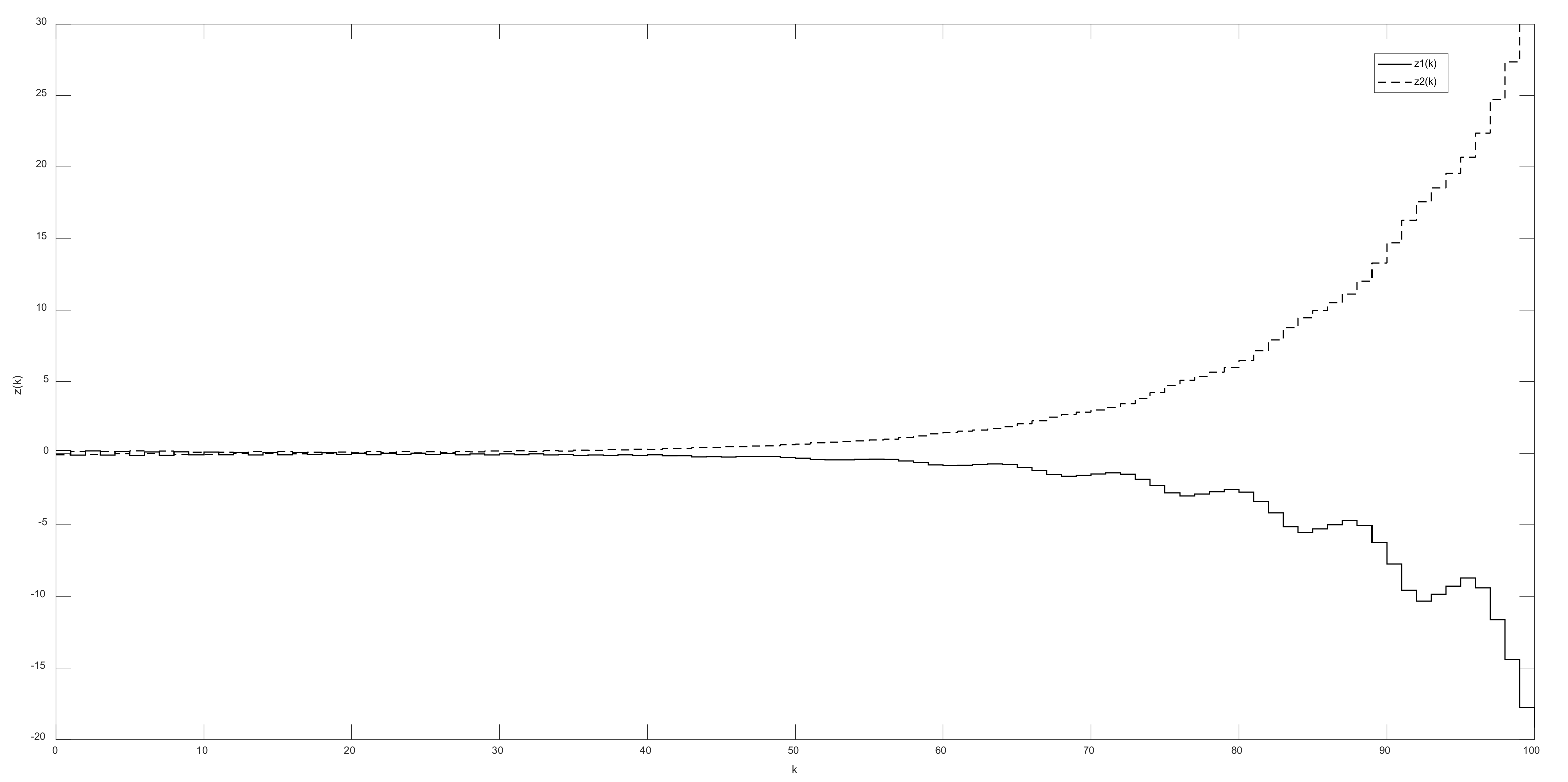
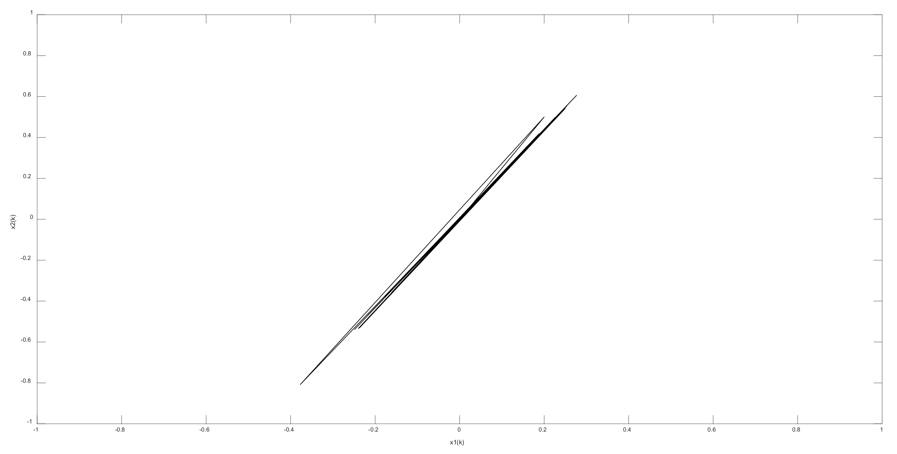
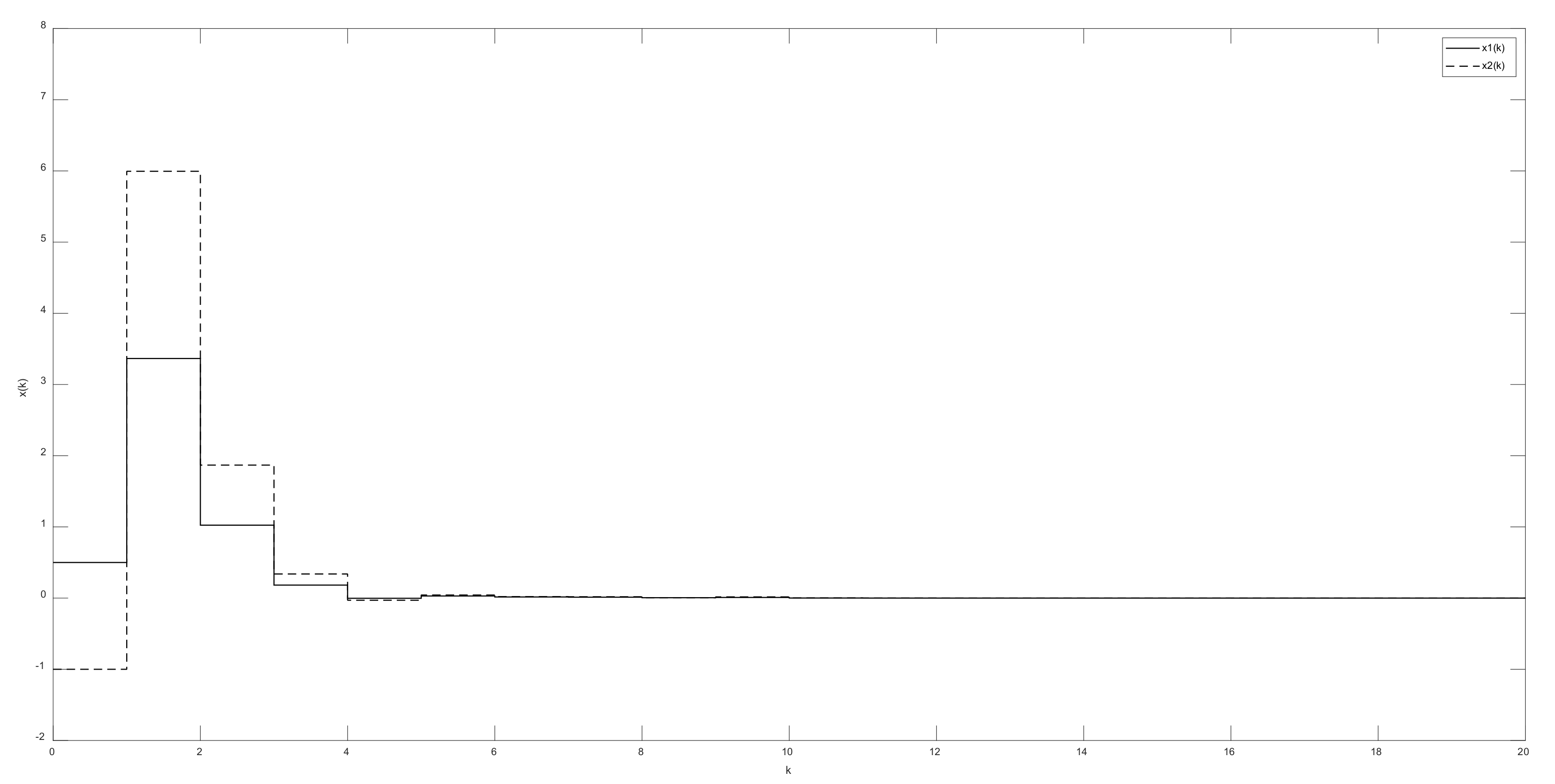
4. Illustrative Examples

Example 1.

Consider the uncertain discrete time-delay system (18) with (19) and the following parameters:

$$\begin{gathered} A_0=\left[\begin{array}{cc}0.4& -0.02\\ -0.3& 0.1\end{array}\right],A_1=\left[\begin{array}{cc}-0.05& 0\\ -0.01& -0.04\end{array}\right],B_{xw}=B_{xu}=\left[\begin{array}{c}0.1\\ 0.5\end{array}\right],A_{z0}=\left[\begin{array}{cc}0.2& 0.1\\ 0& 0.1\end{array}\right], \\ {A}_{z1}=\left[\begin{array}{cc}0.1& -0.1\\ 0.1& 0.2\end{array}\right],B_{zw}=B_{zu}=\left[\begin{array}{c}0.1\\ -0.1\end{array}\right],M_x=\beta ·\left[\begin{array}{cc}0.1& 0\\ 0& 0.2\end{array}\right],M_z=\beta ·\left[\begin{array}{cc}0.2& 0\\ 0& 0.1\end{array}\right], \\ {N}_0=\beta ·\left[\begin{array}{cc}0.1& 0.1\\ 0& 0.1\end{array}\right],N_1=\beta ·\left[\begin{array}{cc}0.1& 0\\ 0.1& 0.1\end{array}\right],N_{2w}=N_{2u}=\beta ·\left[\begin{array}{c}0.1\\ 0\end{array}\right],N_3=\beta ·\left[\begin{array}{cc}0.1& 0\\ 0.1& 0.1\end{array}\right], \\ {N}_4=\beta ·\left[\begin{array}{cc}0.1& 0\\ 0& 0.1\end{array}\right],N_{5w}=N_{5u}=\beta ·\left[\begin{array}{c}0\\ 0.1\end{array}\right],{\Xi }_1={\Xi }_2=0, \\ \overline{\varphi }=\left[{\varphi }^T\left(0\right){\varphi }^T\left(-1\right){\varphi }^T\left(-2\right)\cdots {\varphi }^T\left(-{\tau }_M\right)\right], \\ {\varphi }^T\left(k\right)=\left[1-1\right],k=-{\tau }_M,\cdots ,0. \end{gathered}$$

(26)

We assume that the peak disturbance is constrained by $\overline{w}=1$ and without perturbations ($\beta =0$). Under ${\tau }_m=1$, ${\tau }_M=4$, and $\mathsf{\lambda }=1$, we have $N=4$ and

$$\begin{gathered} E_1=\left[0_{2\times 2}{I}_2{0}_{2\times 2}{0}_{2\times 2}{0}_{2\times 2}\right],E_2=\left[0_{2\times 2}{0}_{2\times 2}{I}_2{0}_{2\times 2}{0}_{2\times 2}\right], \\ {E}_3=\left[0_{2\times 2}{0}_{2\times 2}{0}_{2\times 2}{I}_2{0}_{2\times 2}\right],E_4=\left[0_{2\times 2}{0}_{2\times 2}{0}_{2\times 2}{0}_{2\times 2}{I}_2\right]. \end{gathered}$$

(27)

The stability analysis, switching control, reachable set, and performance of system (18) with (19) and (26) without perturbation ($\beta =0$) and with perturbations ($\beta =1$) are investigated in the following conditions.

Condition (1):

Stability analysis without perturbations, $\beta =0$. With the selection ${\alpha }_0=0.5$, the optimization in (17) of Corollary 1 can be formulated as follows:

Step 1. With ${\delta }_1={\delta }_3={\delta }_4=1000$ and ${\delta }_2=0.55$, a feasible solution can be found.

Step 2. We minimize the value $\overline{\gamma }$; a feasible solution can be found with $\overline{\gamma }=0.1501$.

Step 3. We minimize the value $\alpha$; a feasible solution can be found with $\alpha =$2.6385.

We can conclude that the system (1) with (2), (7), and (26) is asymptotically stable with $H_2$ measure $\alpha =2.6385$ and $H_{\infty }$ performance $\gamma =\sqrt{\overline{\gamma }}=0.3874$, and the reachable set is bounded by hyper-sphere $S\left(a\right)$ with $a=0.55$.

Condition (2):

Stability analysis with perturbations, $\beta =1$. With the selection ${\alpha }_0=0.5$, the optimization in (17) of Corollary 1 can be formulated as follows:

Step 1: With ${\delta }_1={\delta }_3={\delta }_4=1000$ and ${\delta }_2=0.601$, a feasible solution can be found.

Step 2: We minimize the value $\overline{\gamma }$; a feasible solution can be found with $\overline{\gamma }=$0.1728.

Step 3: We minimize the value $\alpha$; a feasible solution can be found with $\alpha =$3.0455.

We can conclude that the system (1) with (2), (7), and (26) is asymptotically stable with $H_2$ measure $\alpha =3.0455$ and $H_{\infty }$ performance $\gamma =\sqrt{\overline{\gamma }}=0.4157$, and the reachable set is bounded by hyper-sphere $S\left(a\right)$ with $a=0.601$.

Condition (3):

Switching control without perturbations,$\beta =0$. With the selection ${\alpha }_{ij}=0.5$, $i,j\in \underset{-}{4}$, the optimization in (23) of Theorem 2 with ${\delta }_2={\delta }_3={\delta }_4=1000$ and ${\delta }_1=0.5296$ in Remark 3 has a feasible solution with $K_i={\check{K}}_i{\check{P}}_{i1}^{-1}$, $i\in \underset{-}{4}$,

$$\begin{gathered} K_1=\left[‒0.3397 0.1445\right],K_2=\left[‒0.4147 0.1839\right], \\ {K}_3=\left[‒0.0206 0.1486\right],K_4=\left[‒0.0568 0.141\right]. \end{gathered}$$

(28a)

By Theorem 2, we can conclude that the system (18) with (7), (19), and (26) is asymptotically stabilizable by the switching control in (20d) with (28a), and the reachable set is bounded by hyper-sphere $S\left(a\right)$ with $a=\underset{i\in N}{\min }{\delta }_i=0.5296$.

Condition (4):

Robust switching control with perturbations, $\beta =1$. With the selection ${\alpha }_{ij}=0.5$, $i,j\in \underset{-}{4}$, the optimization in (23) of Theorem 2 with ${\delta }_2={\delta }_3={\delta }_4=1000$ and ${\delta }_1=0.5773$ in Remark 3 has a feasible solution with $K_i={\check{K}}_i{\check{P}}_{i1}^{-1}$, $i\in \underset{-}{4}$,

$$\begin{gathered} K_1=\left[‒0.2870 0.1557\right],K_2=\left[‒0.3719 0.2025\right], \\ {K}_3=\left[0.2544 0.1125\right],K_4=\left[0.1951 0.971\right]. \end{gathered}$$

(28b)

By Theorem 2, we can conclude that the system (18) with (7), (19), and (26) is asymptotically stabilizable by the switching control in (20d) with (28b), and the reachable set is bounded by hyper-sphere $S\left(a\right)$ with $a=\underset{i\in N}{\min }{\delta }_i=0.5773$.

Condition (5):

Mixed performance switching control without perturbations,$\beta =0$. By Condition (3), Theorem 2, and Corollary 2 with the switching control gains in (28a), we can conclude that the system (18) with (7), (19), and (26) is asymptotically stabilizable with $H_2$ measure $\alpha =3.1908$ and $H_{\infty }$ performance $\gamma =\sqrt{\overline{\gamma }}=0.3841$ by the switching control in (20d) with $K_i$ in (28a), and the reachable set is bounded by hyper-sphere $S\left(a\right)$ with $a=\underset{i\in N}{\min }{\delta }_i=0.5296$.

Condition (6):

Robust mixed performance switching control with perturbations, $\beta =1$. By Condition (4), Theorem 2, and Corollary 2 with the switching control gains in (28b), we can conclude that the system (18) with (7), (19), and (26) is asymptotically stabilizable with $H_2$ measure $\alpha =4.4223$ and $H_{\infty }$ performance $\gamma =\sqrt{\overline{\gamma }}=0.411$ by the switching control in (20d) with $K_i$ in (28a), and the reachable set is bounded by hyper-sphere $S\left(a\right)$ with $a=\underset{i\in N}{\min }{\delta }_i=0.5773$.

With the above conditions (5) and (6), the switching controls in (20d) with (28a) and (28b) can used to improve the reachable set and $H_{\infty }$ performance $\gamma$. The $H_2$ measure $\alpha$ may produce more conservative results with than without switching control. Some comparisons are made in

Table 1. Some comparisons regarding the proposed results of system (1) or (18) with (7) and (28).

Some Comparisons Regarding System (1) or (18) with (7) and (28)
Results	Interval Time-Varying Delay	Conditions	Reachable Set and Performance
[6]	$1\le \tau \left(k\right)\le 4$	No perturbations ($\beta =0$) and no control	$S\left(0.8402\right)$
[4]			$S\left(0.57\right)$
The proposed results in this paper			$S\left(0.55\right)$ $H_2$ measure $\alpha =2.6385$ $H_{\infty }$ performance $\gamma =0.3874$
		$\beta =1$ and no control	$S\left(0.601\right)$ $H_2$ measure $\alpha =3.0455$ $H_{\infty }$ performance $\gamma =0.4157$
		No perturbations ($\beta =0$) Switched control in (20d) with (27a)	$S\left(0.5296\right)$ $H_2$ measure $\alpha =3.1908$ $H_{\infty }$ performance $\gamma =0.3841$
		$\beta =1$ Switched control in (20d) with (27b)	$S\left(0.5773\right)$ $H_2$ measure $\alpha =4.4223$ $H_{\infty }$ performance $\gamma =0.411$

.

Example 2.

Consider the uncertain discrete time-delay system (18) with (19) and the following parameters:

$$\begin{gathered} A_0=\left[\begin{array}{cc}0.9& -0.01\\ -0.2& 1\end{array}\right],A_1=\left[\begin{array}{cc}-0.03& 0\\ -0.02& -0.03\end{array}\right],B_{xw}=B_{xu}=\left[\begin{array}{c}0.2\\ 0.5\end{array}\right],A_{z0}=\left[\begin{array}{cc}0.1& 0.1\\ 0& 0.1\end{array}\right], \\ {A}_{z1}=\left[\begin{array}{cc}0.1& -0.1\\ 0.1& 0.1\end{array}\right],B_{zw}=B_{zu}=\left[\begin{array}{c}0.2\\ -0.1\end{array}\right],M_x=\beta ·\left[\begin{array}{cc}0.01& 0\\ 0& 0.1\end{array}\right],M_z=\beta ·\left[\begin{array}{cc}0.1& 0\\ 0& 0.1\end{array}\right], \\ {N}_0=\beta ·\left[\begin{array}{cc}0.1& 0\\ 0& 0.1\end{array}\right],N_1=\beta ·\left[\begin{array}{cc}0.1& 0.1\\ 0.1& 0.1\end{array}\right],N_{2w}=N_{2u}=\beta ·\left[\begin{array}{c}0.1\\ 0.1\end{array}\right],N_3=\beta ·\left[\begin{array}{cc}0.1& 0.1\\ 0.1& 0.1\end{array}\right], \\ {N}_4=\beta ·\left[\begin{array}{cc}0.1& 0\\ 0& 0.1\end{array}\right],N_{5w}=N_{5u}=\beta ·\left[\begin{array}{c}0\\ 0.1\end{array}\right],{\Xi }_1={\Xi }_2=0, \\ \overline{\varphi }=\left[{\varphi }^T\left(0\right){\varphi }^T\left(-1\right){\varphi }^T\left(-2\right)\cdots {\varphi }^T\left(-{\tau }_M\right)\right],{\varphi }^T\left(k\right)=\left[0.5-1\right],-{\tau }_M,\cdots ,0. \end{gathered}$$

(29)

We assume that the peak disturbance is constrained by $\overline{w}=1$ and without perturbations ($\beta =0$). Under ${\tau }_m=1$, ${\tau }_M=4$, and $\mathsf{\lambda }=1$, we have $N=4$, and $E_i$, $i\in \underset{-}{4}$, are given in (27). With these parameters in (29) and the LMI conditions in Theorem 1 and Corollary 1, we cannot find any feasible solution. Hence, the switching control scheme in (20d) can be considered to stabilize the uncertain discrete system in (18) with (7), (19), (29), and $1\le \tau \left(k\right)\le 4$.

Condition (1):

Mixed performance switching control without perturbations, $\beta =0$. With the selection ${\alpha }_{ij}=0.5$, $i,j\in \underset{-}{4}$, the optimization in (23) of Theorem 2 with ${\delta }_2={\delta }_3={\delta }_4=1000$ and ${\delta }_1=$1.5874 has a feasible solution with $K_i={\check{K}}_i{\check{P}}_{i1}^{-1}$, $i\in \underset{-}{4}$,

$$\begin{gathered} K_1=\left[‒9.5195 6.639\right],K_2=\left[‒9.2945 6.5321\right], \\ {K}_3=\left[‒13.8289 8.8495\right],K_4=\left[‒12.0857 7.9565\right]. \end{gathered}$$

(30)

We can conclude that the system (18) with (7), (19), and (29) is asymptotically stabilizable by the switching control in (20d) with (30), and the reachable set is bounded by hyper-sphere $S\left(a\right)$ with $a=\underset{i\in N}{\min }{\delta }_i=1.5874$. By Corollary 2 with the switching control gains in (30), we can conclude that the system (18) with (7), (19), and (29) is asymptotically stabilizable with $H_2$ measure $\alpha =$93.6876 and $H_{\infty }$ performance $\gamma =\sqrt{\overline{\gamma }}=0.7559$ by the switching control in (20d) with $K_i$ in (30), and the reachable set is bounded by hyper-sphere $S\left(a\right)$ with $a=\underset{i\in \underset{-}{N}}{\min }{\delta }_i=1.5874$.

Condition (2):

Robustmixedperformanceswitchingcontrolwithperturbations,$\beta =1$. With the selection ${\alpha }_{ij}=0.5$, $i,j\in \underset{-}{4}$, the optimization in (23) of Theorem 2 with ${\delta }_2={\delta }_3={\delta }_4=1000$ and ${\delta }_1=$ 1.6362 has a feasible solution with $K_i={\check{K}}_i{\check{P}}_{i1}^{-1}$, $i\in \underset{-}{4}$,

$$\begin{gathered} K_1=\left[‒9.4443 6.5983\right],K_2=\left[‒9.2625 6.5321\right], \\ {K}_3=\left[‒12.4740 8.1607\right],K_4=\left[‒12.2241 8.0382\right]. \end{gathered}$$

(31)

We can conclude that the system (18) with (7), (19), and (29) is asymptotically stabilizable by the switching control in (20d) with (31), and the reachable set is bounded by hyper-sphere $S\left(a\right)$ with $a=\underset{i\in N}{\min }{\delta }_i=1.6362$. By Corollary 2 with the switching control gains in (30), we can conclude that the system (18) with (7), (19), and (29) is asymptotically stabilizable with $H_2$ measure $\alpha =$85.0073 and $H_{\infty }$ performance $\gamma =\sqrt{\overline{\gamma }}=0.7708$ by the switching control in (20d) with $K_i$ in (31), and the reachable set is bounded by hyper-sphere $S\left(a\right)$ with $a=\underset{i\in N}{\min }{\delta }_i=1.6362$.

Under no perturbations, no initial conditions, and the disturbance inputs $w\left(k\right)=1\times {\left(-0.95\right)}^k$ shown in Figure 1, the regulated outputs $z\left(k\right)\in {\Re }^2$ of the discrete system (18), (19), and (29) without control and with switching control (20d) with (30) are shown in Figure 2 and Figure 3, respectively. Figure 3 shows the good disturbance attenuation effect with $H_{\infty }$ performance $\gamma =0.7708$ for switching control (20d) with (30). The state trajectories $x\left(k\right)\in {\Re }^2$ and reachable set with switching control (20d) with (30) are shown in Figure 4 and Figure 5, respectively. Under zero disturbance and initial state function ${\varphi }^T\left(k\right)=\left[0.5-1\right]$, $k=-4,\cdots ,0$, the state trajectories $x\left(k\right)\in {\Re }^2$ and regulated outputs of system (18), (19), and (29) with switching control (20d) with (30) are shown in Figure 6 and Figure 7, respectively. The $H_2$ measure can be observed to be guaranteed in Figure 7. The interval time-varying delay used in this paper is depicted in Figure 8.

With the above conditions (1) and (2), the switching controls in (20d) with (28a) and (28b) can used to improve the reachable set and $H_{\infty }$ performance $\gamma$. The $H_2$ measure $\alpha$ may produce more conservative results with than without switching control. Some comparisons are made in

Table 2. Some comparisons regarding the proposed results of system (1) or (18) with (7) and (29).

Some Comparisons Regarding System (1) or (18) with (7) and (29)
Results	Interval Time-Varying Delay	Conditions	Reachable Set and Performance
[6]	$1\le \tau \left(k\right)\le 4$	No perturbations ($\beta =0$) and no control	Fail
[4]			Fail
The proposed results in this paper		No perturbations ($\beta =0$) Switched control in (20d) with (30)	$S\left(1.5874\right)$ $H_2$ measure $\alpha =93.6876$ $H_{\infty }$ performance $\gamma =0.7559$
		$\beta =1$ Switched control in (20d) with (31)	$S\left(1.6362\right)$ $H_2$ measure $\alpha =85.0073$ $H_{\infty }$ performance $\gamma =0.7708$

5. Conclusions

In this paper, the mixed $H_2$/$H_{\infty }$ performance control and reachable set of uncertain discrete systems with interval time-varying delay and linear fractional perturbations were investigated. Some LMI-based conditions were proposed to guarantee the mixed performance and reachable set of the system under consideration. When the interval time-varying delay has a slow variation condition, the proposed results will be less conservative. Our numerical simulations showed that our proposed method may yield better and more flexible results than those in past research.

References

1. Gu, K.; Kharitonov, V.L.; Chen, J. Stability of Time-Delay Systems; Birkhauser: Boston, MA, USA, 2003. [Google Scholar]
2. Hale, J.K.; Verduyn Lunel, S.M. Introduction to Functional Differential Equations; Springer: New York, NY, USA, 1993. [Google Scholar]
3. Kolmanovskii, V.B.; Myshkis, A. Introduction to the Theory and Applications of Functional Differential Equations; Kluwer Academic Publishs: Dordrecht, The Netherlands, 1999. [Google Scholar]
4. Chen, Y.; Lam, J.; Cui, Y.; Kwok, K.W. Switched systems approach to state bounding for time delay systems. Inf. Sci. 2018, 465, 191–201. [Google Scholar] [CrossRef]
5. Lien, C.H.; Yu, K.W.; Lin, Y.F.; Chung, Y.J.; Chung, L.Y.; Chen, J.D. Exponential stability analysis for uncertain switched neutral systems with interval time-varying state delay. Nonlinear Anal. Hybrid Syst. 2009, 3, 334–342. [Google Scholar] [CrossRef]
6. That, N.D.; Nam, P.T.; Ha, Q.P. Reachable set bounding for linear discrete-time systems with delays and bounded disturbances. J. Optim. Theory Appl. 2013, 157, 96–107. [Google Scholar] [CrossRef]
7. Tunç, C.; Tunç, O.; Wang, Y.; Yao, J.C. Qualitative analyses of differential systems with time-varying delays via Lyapunov–Krasovski approach. Mathematics 2021, 9, 1196. [Google Scholar] [CrossRef]
8. Mahmoud, M.S. Switched Time-Delay Systems; Springer: Boston, MA, USA, 2010. [Google Scholar]
9. Sun, Z.; Ge, S.S. Stability Theory of Switched Dynamical Systems; Springer: London, UK, 2011. [Google Scholar]
10. Baldi, S.; Xiang, W. Reachable set estimation for switched linear systems with dwell-time switching. Nonlinear Anal. Hybrid Syst. 2018, 29, 20–33. [Google Scholar] [CrossRef] [Green Version]
11. Chen, G.; Xiang, G.; Karimi, H.R. Observer-based robust H control for switched stochastic systems with time-varying delay. Abstr. Appl. Anal. 2013, 2013, 320703. [Google Scholar] [CrossRef]
12. Chen, Y.; Lam, J.; Zhang, B. Estimation and synthesis of reachable set for switched linear systems. Automatica 2016, 63, 122–132. [Google Scholar] [CrossRef]
13. Lien, C.H.; Yu, K.W.; Hsieh, J.G.; Chung, L.Y.; Chen, J.D. Simple switching signal design for H performance and control of switched time-delay systems. Nonlinear Anal. Hybrid Syst. 2018, 29, 203–220. [Google Scholar] [CrossRef]
14. Sun, X.M.; Wang, W.; Liu, G.P.; Zhao, J. Stability analysis for linear switched systems with time-varying delay. IEEE Trans. Syst. Man Cybern. B 2008, 38, 528–533. [Google Scholar]
15. Yu, K.W.; Lien, C.H.; Chang, H.C. H analysis and switching control for uncertain discrete switched time-delay systems by discrete Wirtinger inequality. Adv. Differ. Equ. 2017, 2017, 349. [Google Scholar] [CrossRef] [Green Version]
16. Chen, H.; Cheng, J.; Zhong, S.; Yang, J.; Kang, W. Improved results on reachable set bounding for linear systems with discrete and distributed delays. Adv. Differ. Equ. 2015, 2015, 145. [Google Scholar] [CrossRef] [Green Version]
17. Fridman, E.; Shaked, U. On reachable sets for linear systems with delay and bounded peak inputs. Automatica 2003, 39, 2005–2010. [Google Scholar] [CrossRef]
18. Xiao, J.; Xu, F. State bounding estimation for a linear continuous-time singular system with time-varying delay. Adv. Differ. Equ. 2019, 2019, 120. [Google Scholar] [CrossRef]
19. Chang, X.H. Robust nonfragile filtering of fuzzy systems with linear fractional parametric uncertainties. IEEE Trans. Fuzzy Syst. 2012, 20, 1001–1011. [Google Scholar] [CrossRef]
20. Jerbi, H.; Kchaou, M.; Boudjemline, A.; Regaieg, M.A.; Aoun, S.B.; Kouzou, A.L. H and Passive Fuzzy Control for Non-Linear Descriptor Systems with Time-Varying Delay and Sensor Faults. Mathematics 2021, 9, 2203. [Google Scholar] [CrossRef]
21. Lien, C.H.; Hou, Y.Y.; Yu, K.W.; Chang, H.C. Aperiodic sampled-data robust H control of uncertain continuous switched time-delay systems. Int. J. Syst. Sci. 2020, 51, 2005–2024. [Google Scholar] [CrossRef]
22. Du, D. Generalized output feedback controller design for uncertain discrete-time switched systems via switched Lyapunov functions. Nonlinear Analy. Theory Methods Appl. 2006, 65, 2135–2146. [Google Scholar] [CrossRef]
23. Karimi, H.R.; Gao, H. Mixed H2/H output-feedback control of second-order neutral systems with time-varying state and input delays. ISA Trans. 2008, 47, 311–324. [Google Scholar] [CrossRef]
24. Kim, J.H. Robust mixed H2/H control of time-varying delay systems. Int. J. Syst. Sci. 2001, 32, 1345–1351. [Google Scholar] [CrossRef]
25. Lien, C.H.; Yu, K.W.; Chang, H.C. Robust mixed performance switching control for uncertain discrete switched systems with time delay. Int. J. Syst. Sci. 2018, 49, 2144–2154. [Google Scholar] [CrossRef]
26. Li, T.; Guo, L.; Sun, C. Robust stability for neural networks with time-varying delays and linear fractional uncertainties. Neurocomputing 2007, 71, 421–427. [Google Scholar] [CrossRef]
27. Yang, J.; Luo, W.; Li, G.; Zhong, S. Reliable guaranteed cost control for uncertain fuzzy neutral systems. Nonlinear Anal. Hybrid Syst. 2010, 4, 644–658. [Google Scholar] [CrossRef]
28. Boyd, S.P.; El Ghaoui, L.; Feron, E.; Balakrishnan, V. Linear Matrix Inequalities in System and Control Theory; SIAM: Philadelphia, PA, USA, 1994. [Google Scholar]
Figure 1. Disturbance inputs of the system (solid line: w k ).
Mathematics 09 02763 g001
Figure 2. Regulated outputs of the system without control (solid line: z 1 k , dashed line: z 2 k ).
Mathematics 09 02763 g002
Figure 3. Regulated outputs of the system under switching control (20d) with K i in (30) (solid line: z 1 k , dashed line: z 2 k ).
Mathematics 09 02763 g003
Figure 4. State trajectories of the system under switching control (20d) with K i in (30) (solid line: x 1 k , dashed line: x 2 k ) .
Mathematics 09 02763 g004
Figure 5. Reachable set of the system under switching control (20d) with K i in (30).
Mathematics 09 02763 g005
Figure 6. State trajectories for the system without disturbance (solid line: x 1 k , dashed line: x 2 k ).
Mathematics 09 02763 g006
Figure 7. Regulated outputs of the system under switching control (20d) with K i in (30) without disturbance (solid line: z 1 k , dashed line: z 2 k ).
Mathematics 09 02763 g007
Figure 8. Interval time-varying delay.
Mathematics 09 02763 g008