Conceptual Coverage Driven by Essential Concepts: A Formal Concept Analysis Approach

Abstract

Formal concept analysis (FCA) is a mathematical theory that is typically used as a knowledge representation method. The approach starts with an input binary relation specifying a set of objects and attributes, finds the natural groupings (formal concepts) described in the data, and then organizes the concepts in a partial order structure or concept (Galois) lattice. Unfortunately, the total number of concepts in this structure tends to grow exponentially as the size of the data increases. Therefore, there are numerous approaches for selecting a subset of concepts to provide full or partial coverage. In this paper, we rely on the battery of mathematical models offered by FCA to introduce a new greedy algorithm, called Concise, to compute minimal and meaningful subsets of concepts. Thanks to its theoretical properties, the Concise algorithm is shown to avoid the sluggishness of its competitors while offering the ability to mine both partial and full conceptual coverage of formal contexts. Furthermore, experiments on massive datasets also underscore the preservation of the quality of the mined formal concepts through interestingness measures agreed upon by the community.

1. Introduction

With the rapid development of 5G, the Internet of Things (IoT), and artificial intelligence (AI) in recent years, increasing numbers of large datasets are becoming available in a wide variety of communities. In this respect, identifying the cohesive structures in these various datasets facilitates the discovery of valuable hidden patterns. Formal concept analysis (FCA) provides a robust mathematical foundation based on lattice theory for identifying the cohesive structures of a social network [1,2]. In social network analysis, we can model the topological information as a bipartite graph; i.e., a graph with two types of vertices and whose links are only between vertices of different types. Then, by identifying the formal concepts (also known as biclusters [3] or bicliques [4]) from bipartite graphs, the network structure is transformed into a concept form, which indicates the relationships hidden in the data. However, it has often been observed that the overwhelming number of formal concepts is an actual burden for valuable data analysis. Indeed, it is of utmost importance to determine a representative subset from this vast set of formal concepts that can be extracted from even modestly sized formal contexts [5,6,7,8]. Hence, the primary problem in FCA is to find a minimal contextual structure that is concise and maintains thestructural consistency.

For a sizable formal context, the number of formal concepts in a concept (Galois) lattice can be vast, and such complexity is often managed by selecting the most interesting concepts according to a particular metric. This issue was the focus of a myriad of works. Of note, Mouakher and Ben Yahia recently proposed the pioneering QualityCover algorithm [7]. The algorithm was mainly guided by the quality of the extracted association that may be drawn from the intent part of the selected formal concepts. More specifically, the aim was to reduce the number of mined patterns to make them manageable for the end users while preserving the quality of the mined knowledge. The main criticism of this algorithm is the running time, especially when handling large datasets. In addition, the algorithm provides only full conceptual coverage, which is not always needed. In this paper, along the same lines, we introduce the greedy and parametrizable algorithm called Concise. We show that Concise is competitive in terms of running time and complexity. The main broad points of the fresh approach that we introduce are as follows:

• Extraction of full and partial conceptual coverage: Our approach finds a minimal subset of formal concepts that fully or partially cover the relations in the formal context. Partial coverage has received considerably less attention than it deserves. The main conclusion drawn is that partial coverage may be an interesting issue to eliminate the “noise” or outliers from an obtained coverage.
• Scalability: Thanks to the introduced theoretical properties, our approach is shown to be very scalable since it is able to process very large datasets with a reasonable running time.
• Quality of the drawn knowledge: Alongside the compactness feature, the new approach highlights worthy statistics for the interestingness measures of stability, separation, and object uniformity.

The remainder of this paper is organized as follows. First, Section 2 provides background on formal concept analysis, and Section 3 gives a brief overview of related work. Then, in Section 4, we thoroughly describe and illustrate our greedy algorithm, called Concise, for the extraction of optimal full and partial coverage of a formal context. Next, in Section 5, we detail the theoretical complexity of our algorithm. Finally, Section 6 presents the empirical study, and the conclusion and future work are given in Section 7.

2. Basic Settings

Formal concept analysis (FCA) and its mathematical foundations [9] have been used as a theoretical basis for various tasks (e.g., [10,11,12]). In our context, we introduce a new approach for extracting full and partial conceptual coverage based on FCA. Let us recall its basic notions.

Definition 1

(Formal Context). A formal context $\mathcal{K}$ = $(\mathcal{O}$, $\mathcal{I}$, $\mathcal{R})$ consists of two sets $\mathcal{O}$ and $\mathcal{I}$ and a binary(incidence)relation $\mathcal{R}$ between $\mathcal{O}$ and $\mathcal{I}$. The elements of $\mathcal{O}$ are called the objects and the elements of $\mathcal{I}$ are called the attributes of the context. In order to express that an object o is in a relation $\mathcal{R}$ with an attribute i, we write $o\mathcal{R}i$ or (o, i)∈$\mathcal{R}$ and read this as “the object o has the attribute i”.

Example 1.

In the remainder, we consider the formal context $\mathcal{K}$ depicted by

Table 1. An example of formal context.

	a	b	c	d	e	f	g	h
1		×					×
2	×		×				×
3				×	×	×	×	×
4	×			×	×	×	×	×
5	×				×	×	×	×
6		×				×	×
7	×					×	×
8	×				×		×
9	×	×	×	×	×	×	×	×

. A small context can be easily represented by a cross table; i.e., by a rectangular table, the rows of which are headed by the object names and the columns headed by the attribute names. A cross (×) in row o and column i means that the object o has the attribute i. Table 1 illustrates the relationship between a set of patients $\mathcal{O}=\{1,2,3,4,5,6,7,8,9\}$ and a set of symptoms $\mathcal{I}$ = $\{a,b,c,d,e,f,g,h\}$.

Definition 2

(Bipartite Graph). A graph $\mathcal{G}=(\mathcal{N},\mathcal{E})$ is a bipartite graph [13] if there is a bipartition $\{\mathcal{U}\cup \mathcal{V}\}$ of $\mathcal{N}$ such that all edges from $\mathcal{E}$ intersect with all elements of the partition; i.e.,

$$\forall e\in \mathcal{E}:e\cap \mathcal{U}\ne \varnothing \wedge e\cap \mathcal{V}\ne \varnothing$$

It may be noticed that formal contexts are closely related to bipartite graphs, where both objects and attributes are nodes in the graph and edges connect each object with its attributes. This link enables us to employ the whole tool-set of FCA to bipartite graphs and vice versa.

Example 2.

Figure 1 illustrates the formal context depicted in Table 1.

An interesting link between the power sets $\mathcal{P}\left(\mathcal{I}\right)$ and $\mathcal{P}\left(\mathcal{O}\right)$ associated with the set of items $\mathcal{I}$ and the set of objects $\mathcal{O}$ is defined as follows:

Definition 3

(Galois Operators). For a set $A\subseteq \mathcal{O}$ of objects we define:

$$A^{\prime }:=\left\{i\in \mathcal{I}\mid (\forall o\in A),(o,i)\in \mathcal{R}\right\}$$

(1)

(the set of attributes common to the objects in A). Correspondingly, for a set B of attributes, we define

$$B^{\prime }:=\left\{o\in \mathcal{O}\mid (\forall DIFaddbegini\in B),(o,i)\in \mathcal{R}\right\}$$

(2)

(the set of objects which have all attributes in B). The operators ${}^{\prime }$ are known as concept-forming (also known as derivator) operators [9,14].

Definition 4

(Support of a pattern). Let $\mathcal{K}$ = $(\mathcal{O}$, $\mathcal{I}$, $\mathcal{R})$ be a formal context and P be a non-empty pattern. The conjunctive support of a pattern P [15], denoted by Supp(P), is equal to the number of objects/items containing all items/objects of P.

$$Supp\left(P\right)=|P^{\prime }|$$

(3)

Definition 5

(Formal Concept). A formal concept  [9] of the context $\mathcal{K}$ = $(\mathcal{O}$, $\mathcal{I}$, $\mathcal{R})$ is a pair $\langle A,B\rangle$, $B\subseteq \mathcal{I}$, $A^{\prime }=B$ and $B^{\prime }=A$. We call A the extent and B the intent of the concept $\langle A,B\rangle$. $\mathfrak{B}(\mathcal{O},\mathcal{I},\mathcal{R})$ denotes the set of all concepts of the context $\mathcal{K}$ = $(\mathcal{O}$, $\mathcal{I}$, $\mathcal{R})$.

Example 3.

According to Table 1, the set of patients $\left\{169\right\}$(we use a separator-free abbreviated form for the sets, e.g., $\left\{169\right\}$ represents the set of items $\{1,6,9\}$) presents the same symptoms $\left\{bg\right\}$. Thus $\langle 169,bg\rangle$ is a formal concept. However, if we consider $\left\{345\right\}$ and their corresponding symptoms $\left\{efgh\right\}$, we do not obtain a formal concept because ${\left\{efgh\right\}}^{\prime }$$\left\{3459\right\}$≠$\left\{345\right\}$.

Less formally, we can say that a formal concept is a set of objects together with the attributes these objects have in common under the restriction that we cannot add an additional attribute without removing an object and we cannot add an additional object without removing an attribute.

Definition 6

(Pseudoconcept). The pseudoconcept [16] associated with the element $(a,b)$, denoted as PC$(a,b)$, is a binary relation computed by obtaining the Cartesian product of the maximal set of attributes fulfilling the object a and the maximal set of objects having attribute b. Formally,

$$PC(a,b)=\{(o,i)\subseteq \mathcal{R}\mid o\in \{b{\}}^{\prime }\wedge i\in \left\{a\right\}{}^{\prime }\}.$$

(4)

Plainly, PC$(a,b)$ is the union of all the formal concepts containing element $(a,b)$. We also define the size of a given pseudoconcept $PC(a,b)$ as follows:

$$Size\left(PC(a,b)\right)=\frac{\left|PC\right(a,b\left)\right|}{{|\left\{a\right\}}^{\prime }{|\times |\left\{b\right\}}^{\prime }|}$$

(5)

Example 4.

With respect to the formal context shown by Table 1, the pseudoconcept associated with element $(3,h)$ is computed as follows:

$$\begin{array}{cc}\hfill PC(3,h)& =\{(o,i)\subseteq \mathcal{R}\mid o\in {\left\{h\right\}}^{\prime }\wedge i\in {\left\{3\right\}}^{\prime }\}\hfill \\ \hfill & =\left\{\right(o,i)\subseteq \mathcal{R}\mid o\in \{3459\}\wedge i\in \{defgh\left\}\right\}\hfill \\ \hfill & =\left\{\right(3,d),(3,e),(3,f),(3,g),(3,h),(4,d),(4,e),(4,f),(4,g),(4,h),\hfill \\ \hfill & (5,e),(5,f),(5,g),(5,h),(9,d),(9,e),(9,f),(9,g),(9,h)\}\hfill \end{array}$$

The corresponding size of $PC(3,h)$ is computed as follows:

$$\begin{array}{c}\hfill Size\left(PC(3,h)\right)=\frac{\left|PC\right(3,h\left)\right|}{\left|\right\{defgh\left\}\right|\times \left|\right\{3459\left\}\right|}=\frac{19}{20}.\end{array}$$

Definition 7

(Object/Attribute Concept). Let $\mathcal{K}=(\mathcal{O},\mathcal{I},\mathcal{R})$ be a formal context with associated concept (Galois) lattice $\mathfrak{B}(\mathcal{O},\mathcal{I},\mathcal{R})$. An object concept and attribute concept were introduced in [9]. Hence, the following mappings were defined:

$$\gamma \left(o\right):=\langle {\left\{o\right\}}^{″},{\left\{o\right\}}^{\prime }\rangle$$

(6)

where γ relates $\mathcal{O}$ to $\mathfrak{B}(\mathcal{O},\mathcal{I},\mathcal{R})$ and associates each object o with anobject concept$\langle A,B\rangle$ where B is the set of all attributes of o and A is the set of all objects having all the attributes of B.

$$\mu \left(i\right):=\langle {\left\{i\right\}}^{\prime },{\left\{i\right\}}^{″}\rangle$$

(7)

Analogously, μ relates $\mathcal{I}$ to $\mathfrak{B}(\mathcal{O},\mathcal{I},\mathcal{R})$ by associating each attribute set i with anattribute concept$\langle A,B\rangle$ where A is the set of all objects of i and B is the set of all attributes valid for all objects of A.

Example 5.

If we consider the table depicted by

Table 2. Another example formal context.

	a	b	c	d	e
1	×			×
2		×	×
3	×			×
4	×	×	×	×
5	×				×
6	×				×

, we can say that the formal concepts $\langle \mathrm{13,456},a\rangle$, $\langle 24,bc\rangle$, $\langle 134,ad\rangle$, and $\langle 56,ae\rangle$ introduce items $\left\{a\right\}$, $\{b,c\}$, and $\left\{d\right\}$, and finally $\left\{e\right\}$, respectively. Conversely, we can also say that $\langle 134,ad\rangle$, $\langle 24,bc\rangle$, $\langle 4,abcd\rangle$ and $\langle 56,ae\rangle$ introduce objects $\{1,3\}$, $\left\{2\right\}$, $\left\{4\right\}$, and $\{5,6\}$, respectively.

Definition 8

(Full/partial conceptual coverage). Given a formal context $\mathcal{K}=(\mathcal{O},\mathcal{I},\mathcal{R})$ and a threshold δ, a conceptual coverage [17] is defined as a set of formal concepts $C_{\mathcal{K}}=\{C_1,C_2,\dots ,C_n\}$ in the concept (Galois) lattice $\mathfrak{B}(\mathcal{O},\mathcal{I},\mathcal{R})$ [9,14].

The conceptual coverage $C_{\mathcal{K}}$ is said to be full $(\delta =1)$ if any element $(x,y)$ in the context $\mathcal{K}$ is included in at least one concept of $C_{\mathcal{K}}$. However, the conceptual coverage is said to be partial $(\delta <1)$ whenever the number of elements $(x,y)$ in $C_{\mathcal{K}}$ covers δ percent of the formal context $\mathcal{K}$.

Example 6.

If we consider the formal context depicted by Table 1 and $\delta =1$, $C_{\mathcal{K}}$=$\{\langle$169, bg〉, 〈349, defgh〉, 〈29, acg〉, 〈245789, ag〉, 〈345679, fg〉, 〈3459, efgh〉, 〈34589, eg$\rangle \}$ is one full coverage since every element is covered by at least one formal concept.

In the following, we present the most relevant works that address the extraction of the full and partial conceptual coverage of a formal context.

3. Related Work

In the literature, extracting the minimal coverage of formal concepts (i.e., the set covering problem) is not entirely new and has been the subject of several previous works. Some of these approaches focused on covering the entire formal context and are called full-coverage approaches, whereas others called partial-coverage approaches were interested in covering only a subset of the formal context.

3.1. Full-Coverage Approaches

Kcherif et al. [18] introduced a rectangular decomposition approach based on Riguet’s difunctional relation. Indeed, computing this difunctional was reduced to detecting a particular set of elements called isolated points, allowing the determination of the minimal conceptual coverage of a given binary relation. Later, an extended isolated points-based approach was applied on textual data in [19]. The authors proposed an algorithm called MinGenCoverage for covering a formal context (as a formal representation of a text) based on isolated labels. The algorithm studied the connections between minimal generators and isolated points, which reduced the search space and improved its performance. Mouakher and Ben Yahia [7] introduced a new approach based on a greedy algorithm called QualityCover to build a full conceptual coverage. The authors defined a new gain function based on correlation metrics for high-quality coverage. The major drawback of this approach is scalability. Another related work is [20] which investigated the same problem using bipartite graphs. The authors proposed a new algorithm called FastCover which provided a concise conceptual coverage using the graph structure. Later, Elloumi et al. relied on the notion of N-composite isolated points to produce the conceptual coverage progressively and proposed a new approach for conceptual coverage construction based on N-composite isolated points [21]. Belohlavek and Vychodil [22] tackled the same issue by attempting to solve the Boolean factor analysis problem. The authors proposed a greedy approximation algorithm, called GreCond, aiming to find approximately optimal decompositions of binary matrices. In the same trend, Belohlavek and Trnecka [23], via the GreEss algorithm, focused on the same issue. Thus, they proposed an approach for decomposing a binary matrix into a Boolean product of factors. Recently, Tatiana and Martin [24] proposed an MDL-based from-below factorization algorithm called MDLGreCond. The algorithm uses the minimum description length (MDL) principle as a criterion for factor selection and produces a small subset of formal concepts with a low information loss rate.

3.2. Partial-Coverage Approaches

The partial coverage approaches have received less attention from the FCA community. To the best of our knowledge, the GreEss algorithm [23], mentioned in the previous subsection, is one of the most well-known approaches allowing generating partial coverage. However, this problem is usually assimilated to a $\delta$ approximation role mining problem, and it is also proven to be NP-complete [25]. In this case, users and permissions correspond to FCA objects and FCA attributes, respectively, and measuring $\delta$ for a selected subset of concepts uses the coverage ratio c to evaluate role mining algorithms  [25]. Some studies have been proposed by the role mining community [25,26]. In [27], the authors addressed the same issue and presented a novel bottom-up approach called the $\delta$-Approx Important Role Mining approach in which the permissions were classified based on the number of users assigned to. It has been shown that this approach is effective in decreasing the number of roles. Torim et al. [28] proposed three heuristic algorithms using concept chains instead of formal concepts for partial context coverage. Their approach was mainly based on the selection of a subset of the most interesting concepts. This study was extended in [8]. The authors proposed a novel concept chain coverage method to service the use data of a telecommunications company. The idea behind concept chain coverage is to cover the data not with single concepts but with chains of related concepts. Recently, Kristo et al. [29] introduced a greedy algorithm for generating efficient partial coverage. The latter algorithm is a revised version of GreCond [22], and the choice of the selected concept is based on minimizing the cumulative coverage.

In this paper, we revisit the QualityCover algorithm [7] and propose an efficient implementation for full and partial conceptual coverage called Concise.

4. The Concise Algorithm: A Conceptual Coverage Driven by Essential Concepts

In this section, we present the description of the Concise algorithm. First, we explain the importance of the essential concepts. Then, we detail the use of these fundamental elements in the pseudocode of the algorithm.

4.1. Essential Formal Concepts

Essential concepts, also called mandatory concepts (MCs), play a crucial role in data mining as they allow the discovery of regular structures from data based on formal concept analysis (FCA). They qualify as essential because they belong to any conceptual coverage of a formal context [22]. From the relational algebra (RA) perspective, an essential concept contains at least one isolated point, as introduced by Riguet [30]. As a mathematical background, FCA and RA have already been combined and used to discover regularities in data [18]. A formal concept represents the regular atomic structure for decomposing a binary relation. Moreover, the computing of Riguet’s difunctional relation [30] results in a set of isolated points describing invariant structures that could be used for database decomposition and textual feature selection (TFS) [19]. Furthermore, an isolated point belongs to a unique formal concept that exists in any conceptual coverage. Therefore, any FCA-based knowledge discovery process necessarily considers such concepts. Several approaches have been proposed to locate the essential concepts in a formal context to build conceptual coverage. This paper presents alternatives for conceptual coverage construction, and we discuss their main characteristics and features. Nevertheless, finding the most efficient strategy remains a challenging perspective.

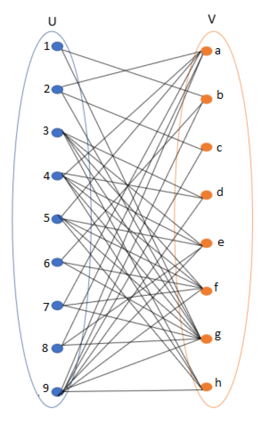
Definition 9

(Isolated Point). Let us consider a formal context $\mathcal{K}$ = $(\mathcal{O},\mathcal{I},\mathcal{R})$. An element $(o,i)\in \mathcal{R}$ is said to be an isolated point if it belongs to only one formal concept.

Definition 10

(Essential Concept). A formal concept is called essential if it contains at least one isolated point.

Theorem 1.

A formal concept $C=\langle A,B\rangle$ is essential if it is both an object concept and an attribute concept.

Proof. 

⇒. Let $\langle A_1,B_1\rangle$ be a formal concept that introduces the objects in a nonempty set $\mathcal{O}$ and the attributes in a nonempty set $\mathcal{I}$. Let $(o,i)\in \mathcal{O}\times \mathcal{I}$. By definition, ${\left\{o\right\}}^{\prime }=B_1$ and ${\left\{i\right\}}^{\prime }=A_1$. Hence, for any formal concept $\langle A_2,B_2\rangle$ such that $o\in A_2$ and $i\in B_2$, we have $A_2\subseteq A_1$ and $B_2\subseteq B_1$. As $\langle A_1,B_1\rangle$ is a formal concept and thus maximal, $A_2=A_1$ and $B_2=B_1$. Consequently, for all $(o,i)\in \mathcal{O}\times \mathcal{I}$, $(o,i)$ only belongs to $\langle A_1,B_1\rangle$, which is consequently essential.

⇐. Let $\langle A_1,B_1\rangle$ be an essential concept and $(o,i)$ be an isolated point that only belongs to $\langle A_1,B_1\rangle$. We find that ${\left\{o\right\}}^{\prime }=B_1$ and ${\left\{i\right\}}^{\prime }=A_1$. This means that $\langle A_1,B_1\rangle$, by definition, introduces both o and i and is thus an object concept and attribute concept.    □

Example 7.

With respect to Table 2, we find the following: $\langle 56,ae\rangle$, $\langle 24,bc\rangle$, and $\langle 134,ad\rangle$ introduce both an object and an attribute and are essential concepts.

Corollary 1.

Let $\mathcal{K}=(\mathcal{O},\mathcal{I},\mathcal{R})$ be a formal context. Let $(o,i)\in \mathcal{R}$ such as $o\in \mathcal{O}$, $i\in \mathcal{I}$. Let $\langle A,B\rangle$ be the associated formal concept to $(o,i)$, where ${\left\{o\right\}}^{″}=A\wedge {\left\{i\right\}}^{″}=B$. The element $(o,i)$ is an isolated point if o is a minimal generator [31] of A and i is a minimal generator of B.

Proof. 

The proof is straightforward since, by definition, a minimal generator is the smallest element for which the closure computation leads to the closed element. Thus, since o and i are minimal generators, which is equivalent to being an object concept and attribute concept, respectively, $(o,i)$ is an isolated point.    □

The following theorem introduces the formal characterization of an isolated point.

Theorem 2.

Let us consider a formal context $\mathcal{K}=(\mathcal{O},\mathcal{I},\mathcal{R})$ and $(o,i)\in \mathcal{R}$. The element $(o,i)$ is an isolated point if ${|\left\{o\right\}}^{″}{|=|\left\{i\right\}}^{\prime }|$.

Proof. 

The proof shows that for an essential formal concept $\langle X,Y\rangle$, an element $(o,i)$ exists such that ${|\left\{o\right\}}^{″}{|=|\left\{i\right\}}^{\prime }|$. Since $o\in X$, then we have ${X\subseteq |\left\{o\right\}}^{″}|$. Moreover, we find ${|\left\{o\right\}}^{″}{|=|\left\{i\right\}}^{\prime }|$, which means that the object exactly generates the extent part X; that is, ${|\left\{o\right\}}^{″}|=X$. In addition, this also means that $i\in Y$ is the only item that appears exactly in the same objects as X. In consequence, i is also a minimal generator of Y.    □

Corollary 2.

Let us consider a formal concept $C=\langle X,Y\rangle$. If $\left|X\right|=1$, then $\langle X,Y\rangle$ is an essential formal concept.

Proof. 

If the extent part is reduced to a singleton, this single object is the object concept of C. Then, the proof that $\exists i\in Y$, such that it is an attribute concept of C—i.e., $(X,i)$ is an isolated point—remains true. Since the cardinality of the extent part of C is equal to 1, it means that this object, say o, fulfills this property, ${\left\{o\right\}}^{\prime }=Y$.    □

Example 8.

According to the formal context given in Table 1, the list of essential concepts can be easily checked: $\{\langle 169,bg\rangle$; $\langle 29,acg\rangle$; $\langle 349,defgh\rangle \}$. If we consider the formal context given by Table 2, all of its formal concepts are essential.

Remark 1.

Let us consider the particular formal context given by

Table 3. A particular formal context with the corresponding formal context of each item.

	a	b	c	d	${|\left\{\mathit{o}\right\}}^{\prime }|$
1	×	×	×		3
2	×			×	2
3		×	×	×	3
4	×	×	×	×	4
$\langle {\left\{i\right\}}^{\prime },{\left\{i\right\}}^{″}\rangle$	$\langle 124,a\rangle$	$\langle 134,bc\rangle$	$\langle 134,bc\rangle$	$\langle 234,d\rangle$

. As this table shows, no essential formal concepts can be mined.

In the following, we provide a formal characterization of the type of formal context, namely the “worst case”, and prove that we cannot mine essential formal concepts from this type of formal context. A “worst case” formal context is defined as follows:

Definition 11.

A “worst case” context is a triplet $\mathcal{K}=(\mathcal{O},\mathcal{I},\mathcal{R})$ where $\mathcal{I}$ is a finite set of items of size n, $\mathcal{O}$ represents a finite set of objects of size $(n+1)$, and $\mathcal{R}$ is a binary (incidence) relation (i.e., $\mathcal{R}$⊆$\mathcal{O}\times \mathcal{I})$. In such a context, each item belongs to n distinct objects. Each object, among the first n objects, contains $(n-1)$ distinct items, and the last object is fulfilled by all items.

Thus, in a “worst case” context, each object concept/attribute concept is equal to its unique minimal generator. Hence, from a “worst case” context of a dimension equal to n×$(n$+$1)$, 2${}^n$ formal concepts can be extracted. Even if the worst case is rarely encountered in practice, “worst case” datasets have been shown to allow the behavior of an algorithm to be scrutinized on extremely sparse concepts and hence to assess its scalability [15].

Table 4. A “worst case” context for $n=4$.

	a	b	c	d
1		×	×	×
2	×		×	×
3	×	×		×
4	×	×	×
5	×	×	×	×

presents an example of a “worst case” dataset for $n=4$.

Corollary 3.

No essential concepts can be extracted from a worst case formal context.

Proof. 

Let us consider a worst case formal context $\mathcal{K}=(\mathcal{O},\mathcal{I},\mathcal{R})$. By constructing a worst case dataset, and with regard to Theorem 2, we have the following assumptions:

• ${\forall o\in \mathcal{O},|\left\{o\right\}}^{″}|=2$
• $\forall i\in \mathcal{I},\left|i\right|=n$

• $\forall (o,i)$, we find always that ${|\left\{o\right\}}^{″}{|\ne |\left\{i\right\}}^{\prime }|$. Thus, no essential concepts can be drawn from a worst case dataset.    □

4.2. Description of the Concise Algorithm

In the following, we present the description and the pseudocode of the Concise algorithm. According to the pseudocode described by Algorithm 1, we start by computing the basic information from the ground set items of the given formal context. Then, this process computes the corresponding formal concept for each item. The different steps followed to obtain minimal conceptual coverage are detailed in the remainder of this section.

Algorithm 1: The Concise algorithm.

The Concise algorithm proceeds according to the following steps:

Step 1: 

Detect the essential concepts

After closing the items through the Compute_Introductory_Closure procedure, the efficient detection of the set of essential formal concepts (if they exist) is conducted by the Compute_Essential_Concepts function. The corresponding pseudocode is provided by Algorithm 2. The algorithm iterates over the seed set of attributes $\mathcal{I}$. In (Lines 4–8) and with regard to Corollary 2, if the cardinality of the extent part is equal to 1, then its induced formal concept is considered an essential concept, and we remove all the covered elements from the formal context. Otherwise, we iterate over the extent part, seeking an object whose support is equal to the cardinality of the intent part (c.f. Lines 12–16). Finally, we run the second and third steps if the essential concepts do not reach the threshold $\delta$ covering the formal context.

Algorithm 2:Compute_Essential_Concepts.

Step 2: 

Compute the size of noncovered elements

For each noncovered element $(o,i)$, we proceed by obtaining its corresponding pseudoconcept through the Get_PseudoConcept function and assessing its size by calling the Compute_Size function (c.f. Lines 10–11). We provide a more straightforward reformulation of the size in the Compute_Size function based on the following corollary.

Corollary 4.

Let us consider the element $(o,i)\in \mathcal{R}$. The size of its corresponding pseudoconcept according to Equation (5) can be rewritten as follows:

$$\mathit{Size}\left(PC(o,i)\right)=\frac{{\sum }_{k\in {\left\{o\right\}}^{\prime }}^{}|{\left\{i\right\}}^{\prime }\cap {\left\{k\right\}}^{\prime }|}{{|\left\{i\right\}}^{\prime }{|\times |\left\{o\right\}}^{\prime }|}=\frac{1}{Supp\left(o\right)}+\frac{{\sum }_{i\ne k\in {\left\{o\right\}}^{\prime }}^{}|{\left\{i\right\}}^{\prime }\cap {\left\{k\right\}}^{\prime }|}{{|\left\{i\right\}}^{\prime }{|\times |\left\{o\right\}}^{\prime }|}.$$

(8)

Example 9.

If we consider the formal context depicted by Table 1, then element $(3,h)$ and its corresponding pseudoconcept $PC(3,h)$ are calculated as

$$\begin{array}{cc}\hfill PC(3,h)& =\{(o,i)\subseteq \mathcal{R}\mid o\in {\left\{h\right\}}^{\prime }\wedge i\in {\left\{3\right\}}^{\prime }\}\hfill \\ \hfill & =\left\{\right(o,i)\subseteq \mathcal{R}\mid o\in \{3459\}\wedge i\in \{defgh\left\}\right\}\hfill \end{array}$$

The size of this pseudoconcept is computed as follows:

$$\begin{array}{cc}\hfill \mathit{Size}\left(PC(3,h)\right)& =\frac{{|\left\{h\right\}}^{\prime }\cap {\left\{d\right\}}^{\prime }{|+|\left\{h\right\}}^{\prime }\cap {\left\{e\right\}}^{\prime }{|+|\left\{h\right\}}^{\prime }\cap {\left\{f\right\}}^{\prime }{|+|\left\{h\right\}}^{\prime }\cap {\left\{g\right\}}^{\prime }{|+|\left\{h\right\}}^{\prime }|}{4\times 5}\hfill \\ \hfill & =\frac{{|\left\{3459\right\}\cap \left\{d\right\}}^{\prime }{|+|\left\{3459\right\}\cap \left\{e\right\}}^{\prime }{|+|\left\{3459\right\}\cap \left\{f\right\}}^{\prime }|}{4\times 5}\hfill \\ \hfill & +\frac{{|\left\{3459\right\}\cap \left\{g\right\}}^{\prime }|+|\left\{3459\right\}|}{4\times 5}=\frac{3+4+4+4+4}{4\times 5}=\frac{19}{20}\hfill \end{array}$$

The following pseudocode given by Algorithm 3 illustrates the Compute_Size function.

Algorithm 3:Compute_Size.

Step 3: 

Greedily cover the remaining concepts

We repeat this algorithm step when the fixed threshold $\delta$ of covered elements (c.f. Line 14) is not reached. Then, for each uncovered element, we call the Calculate_Best_FC function (c.f. Line 17) to obtain the best candidate to add to the concept coverage. This best candidate is selected according to a quality metric. In the Calculate_Best_FC function, we use the bond measure [32], and the chosen concept is the concept that maximizes this measure. This correlation measure computes the ratio between the conjunctive support and the disjunctive support. In [7], it was shown that this metric results in formal concepts with high quality. The bond measure of a nonempty pattern $I\subseteq \mathcal{I}$ is defined as follows:

$$Bond\left(I\right)=\frac{Supp(\wedge I)}{Supp(\vee I)}.$$

If we consider the formal concept $C=\langle X,Y\rangle$, the formula of the bond can be expressed as follows:

$$Bond\left(Y\right)=\frac{\mid X\mid }{max\left\{Supp\right(o)\mid o\in X\}}.$$

(9)

Equation (9) shows that for a formal concept $C=\langle X,Y\rangle$ such that $\left|Y\right|=1$, we have $Bond\left(C\right)>Bond\left(C^{\prime }\right)$ s.t. $C^{\prime }\ne C$ and $C^{\prime }\in PC(o,Y)\forall o\in X$.

Therefore, if the cardinality of the intent part is equal to 1, then it is the best formal concept, in terms of the bond metric, from all the formal concepts included in the pseudoconcept induced by element $(o,i)$.

Algorithm 4 describes the pseudocode of the Calculate_Best_FC function. As outlined by Line 3, we have to explore ${|\left\{o\right\}}^{\prime }|$ formal concepts exactly. Indeed, it is useless to explore all the formal concepts obtained by combining the seed attributes. From them, we will return the best concept in terms of the bond measure. We do not need to generate the formal concepts since we can decide on their extent. Then, we assess the bond metric value of each generated concept using Equation (9) (c.f. Line 7). The formal concept having the highest bond value is the returned $BestFc$ (c.f. Line 10).

Algorithm 4:Calculate_BestFC.

Example 10.

In this example, we illustrate the different phases of theConcisealgorithm for building minimal conceptual coverage. Let us consider the formal context $\mathcal{K}$ given by Table 1 with a threshold δ = 1. The procedure of the algorithm is depicted in

Table 5. The procedure of the Concise algorithm ($\delta$ = 1) on the formal context given by Table 1.

Iteration	Element	Size	BestFC	Removed from $\mathcal{K}$
Iteration 1	$(1,b)$	1	$\langle 169,bg\rangle$	$(1,b),(1,g),(6,b),(6,g),(9,b),(9,g)$
Iteration 2	$(2,c)$	1	$\langle 29,acg\rangle$	$(2,a),(2,c),(2,g),(9,a),(9,c)$
Iteration 3	$(3,d)$	1	$\langle 349,defgh\rangle$	$(3,d),(3,e),(3,f),(3,g),(3,h),(4,d),(4,e),(4,f),$$(4,g),(4,h),(9,d),(9,e),(9,f),(9,h)$
Iteration 4	$(5,h)$	$\frac{19}{20}$	$\langle 3459,efgh\rangle$	$(5,e),(5,f),(5,g),(5,h)$
Iteration 5	$(8,e)$	$\frac{14}{15}$	$\langle \mathrm{34,589},eg\rangle$	$(8,e),(8,g)$
Iteration 6	$(7,a)$	$\frac{16}{18}$	$\langle \mathrm{245,789},ag\rangle$	$(4,a),(5,a),(7,a),(7,g),(8,a)$
Iteration 7	$(7,f)$	$\frac{16}{18}$	$\langle \mathrm{345,679},fg\rangle$	$(6,f),(7,f)$

.

Step 1: During this step, we first call the Compute_Introductory_Closure procedure, and we obtain

Table 6. The formal context given by Table 1 with additional information.

	a	b	c	d	e	f	g	h	${|\left\{\mathit{o}\right\}}^{\prime }|$
1		×					×		2
2	×		×				×		3
3				×	×	×	×	×	5
4	×			×	×	×	×	×	6
5	×				×	×	×	×	5
6		×				×	×		3
7	×					×	×		3
8	×				×		×		3
9	×	×	×	×	×	×	×	×	8
${\left\{i\right\}}^{\prime }$	245,789	169	29	349	34,589	345,679	123,456,789	3459
${\left\{i\right\}}^{″}$	$ag$	$bg$	$acg$	$defgh$	$eg$	$fg$	g	$efgh$

. Then, we invoke the Compute_Essential_Concepts function, and we find that $(1,b)$, $(2,c)$, $(3,d)$ are isolated points. Thus, we have three essential formal concepts and $C_{\mathcal{K}}=\{\langle 169,bg\rangle ,\langle 29,acg\rangle ,\langle 349,defgh\rangle \}$. Since $\mathcal{K}$ does not fully cover $(\delta$ = $1)$, we proceed to the second step.

Step 2: In this step, we compute the pseudoconcept of elements in the formal concept by invoking the Get_PseudoConcept function. Next, the size of each pseudoconcept is assessed through the Compute_Size function. Then, the elements are sorted in decreasing order via the Sort_Elements procedure.

Step 3: The different outputs obtained during this step are also detailed in Table 5. After sorting the elements, we find that $(3,h)$ and $(5,h)$ are ranked first with a size value equal to $\frac{19}{20}$. Since element $(3,h)$ has already been covered by an essential concept, the best formal concept is $\langle 3459,efgh\rangle$. Thus, we update the list of concept coverage as follows: ${\mathcal{C}}_{\mathcal{K}}=\{\langle 169,bg\rangle$, $\langle 29,acg\rangle$, $\langle 349,defgh\rangle$, $\langle 3459,efgh\rangle \}$. All the elements covered by this list of formal concepts are removed from the initial list. Then, element $(8,e)$ with a size value equal to $\frac{14}{15}$ comes into play, and the formal concept $\langle 34589,eg\rangle$ is added to $C_{\mathcal{K}}$. Then, element $(7,a)$ with a size value equal to $\frac{16}{18}$ comes to the top. Consequently, the formal concept $\langle 245789,ag\rangle$ is added to $C_{\mathcal{K}}$, and the latter becomes equal to ${\mathcal{C}}_{\mathcal{K}}=\{\langle 169,bg\rangle$, $\langle 29,acg\rangle$, $\langle 349,defgh\rangle$, $\langle 3459,efgh\rangle$, $\langle 34589,eg\rangle$, and $\langle 245789,ag\rangle \}$. After removing the covered elements, we find on the top of the remaining elements the couple $(7,f)$(as shown by Table 5). The best concept obtainable from the latter is $\langle 345679,fg\rangle$. Thanks to the latter formal concept, all the elements of the formal context are covered, and the final cover of 7 formal concepts is as follows: ${\mathcal{C}}_{\mathcal{K}}=\{\langle 169,bg\rangle$, $\langle 29,acg\rangle$, $\langle 349,defgh\rangle$, $\langle 3459,efgh\rangle$, $\langle 34589,eg\rangle$, $\langle 245789,ag\rangle$, $\langle 345679,fg\rangle \}$.

5. Theoretical Complexity

We now derive an upper bound of the worst-case time complexity of the Concise algorithm. First, let us denote n, m, and k as the numbers of objects, items, and entries, respectively, with × of the input formal context $\mathcal{K}$. To simplify the analysis, we assume that $max(n,m)\le k$, which is a reasonable condition. Moreover, computing ${\left\{o\right\}}^{\prime }$${\left\{i\right\}}^{\prime }$ takes $O\left(m\right)$ and $O\left(n\right)$ time, respectively. Therefore, the complexity of the Compute_Introductory_Closure procedure is estimated by $n\times O\left(n\right)$. The complexity of the Compute_Essential_Concepts function is $n\times \left(O\right(n)+O(m\left)\right)$. Then, the Get_PseudoConcept and the Compute_Size functions can be performed in $O(n·m)$ time in the worst case. The cost of these functions in the loop (Lines $8-11$) is $n\times O(n·m)$. We have chosen the Quicksort algorithm to sort elements $(o,i)$ of the formal context with respect to the size of the associated pseudoconcepts. This sort has a complexity of $O(n·log(n\left)\right)$ according to [33]. The number of elements in the formal context is equal to k. Thus, there are k possible iterations in the case of full coverage, i.e., $(\delta =1)$. The Calculate_Best_FC function takes $n\times \left(O\right(n)+O(m\left)\right)$ in the worst case. In summary, we can say that the theoretical complexity of the Concise algorithm is polynomial, which is equal to $O\left(k^2\right)$.

6. Experimental Evaluation

In this section, we present our results, showing the efficiency of our proposed algorithm. The solution was implemented and executed on a machine with 32 cores, 64 GB of memory and an Ubuntu Linux operating system. The CPUs are modern and have the AVX-512 instructions available, which can provide more than 10-fold increases in speed in some data processing tasks.

6.1. Benchmark Datasets

In this study, we used some benchmark datasets for experimental investigations of the performance and robustness of our proposed algorithm. As shown in

Table 7. The benchmark datasets ordered by the number of formal concepts.

Dataset	# Objects	# Attributes	# Concepts
Apj	2044	1164	797
DBLP	6980	19	2494
Americas-small	3477	1587	2763
DNA	4590	392	4482
Breast-cancer	699	110	9860
Paleo	501	139	10,224
Houses-votes	435	18	10,642
Spect-test	187	23	14,532
Americas-large	3485	10,127	36,990
Tic-tac-toe	958	30	59,504
Mushroom	8124	119	238,710
Soybean-large	307	133	806,030
Dermatology	366	130	1,484,088
Chess	3196	76	930,851,336
Dual-matching-40	1,048,576	40	3,486,784,401
Ac-90k	4322	337	6,801,048,023

, we considered the Apj and Americas-small datasets. The remaining datasets were furnished by the UC Irvine Machine Learning Database Repository [34]. The table presents the number of objects, the number of attributes, and the number of all formal concepts that may be drawn from the dataset using the Lcm algorithm [35] for each dataset. The datasets are listed in increasing order with regard to the number of formal concepts.

6.2. Performance of the Concise Algorithm

In the following, we evaluate the Concise algorithm. In the first step, we compare the minimal coverage (or compacity) with the GreEss. In fact, according to [7], the latter generates the best coverages in terms of compacity. Then, we assess the quality of full and partial converges using different metrics.

Definition 12

(Stress). Stress measures the conciseness of the presentation of a matrix (two-mode data) and can be seen as a purity function that compares the values in a matrix with their neighbors. The stress measures used here are computed as the sum of squared distances of each matrix entry from its adjacent entries. In [36], Niermann defined two types of neighborhoods for an n × m matrix $X=\left(x_{ij}\right)$:

• The Moore neighborhood (M Stress) comprises the (at most) eight adjacent entries. The local stress measure for element x${}_{ij}$ is defined as

  $$M_{ij}=\sum _{k=max(1,i-1)}^{min(n,i+1)}\sum _{l=max(1,j-1)}^{min(m,j+1)}{(x_{ij}-x_{kl})}^2.$$

  (10)
• The Neumann neighborhood (N Stress) comprises the (at most) four adjacent entries resulting in the local stress of x${}_{ij}$:

  $$N_{ij}=\sum _{k=max(1,i-1)}^{min(n,i+1)}{(x_{ij}-x_{kj})}^2+\sum _{l=max(1,j-1)}^{min(m,j+1)}{(x_{ij}-x_{il})}^2.$$

  (11)

As depicted by

Table 8. Comparison between Concise and GreEss algorithms on the criterion of the coverage minimality. (–) means that we were unable to obtain a result after 48 h.

Dataset	# Concepts	N Stress	M Stress	Concise	GreEss
Apj	797	0.003	0.002	474	453
DBLP	2494	0.196	0.414	19	19
Americas-small	2763	0.008	0.024	217	178
DNA	4482	0.013	0.034	377	372
Breast-cancer	9860	0.152	0.329	92	107
Paleo	10,224	0.075	0.160	144	145
Houses-votes	10,642	0.432	0.909	18	27
Spect-test	14,532	0.377	0.797	24	26
Americas-large	36,990	0.013	0.029	636	–
Tic-tac-toe	59,504	0.394	0.931	29	32
Mushroom	238,710	0.249	0.566	110	105
Soybean-large	806,030	0.327	0.795	103	126
Dermatology	1,484,088	0.342	0.773	128	158
Chess	930,851,336	0.461	1.258	72	113
Dual-matching-40	1,048,576	0.397	1.120	40	–
Ac-90k	6,801,048,023	0.025	0.065	37	–

, the Concise algorithm gives equal or more compact coverages than the GreEss algorithm on 12 out of 16 datasets. Furthermore, for the Soybean-large and Dermatology datasets, Concise outputs 103 and 128 formal concepts, respectively, while GreEss flags 126 and 158 formal concepts, respectively. A close look at Table 8 reveals that Concise performs better than GreEss (except with the Mushroom dataset) when N stress and M stress are higher. Although the GreEss algorithm outperforms Concise for some datasets, the latter could not provide results for Americas-large, Dual-matching-40, and Ac-90k datasets.

Comparison between the Full and Partial Coverage of the Concise Algorithm

The principal added value of the Concise algorithm is that it provides full and partial coverage of formal concepts using a threshold $\delta$. We evaluate the obtained coverage regarding the number of concepts, quality metrics, and running time below.

The impact of the variation of $\delta$ on the number of concepts obtained by the Concise algorithm is shown in Figure 2 and

Table 9. The number of concepts of the Concise algorithm with different thresholds.

Datasets	Threshold $\mathit{\delta }$
	100%	90%	80%	70%	60%	50%
Apj	774	321	239	188	156	140
DBLP	19	15	12	10	8	6
Americas-small	217	52	44	42	42	42
DNA	377	208	158	124	100	82
Breast-cancer	92	51	33	21	14	10
Paleo	144	108	89	76	66	56
Houses-votes	18	16	14	12	10	8
Spect-test	24	19	16	13	11	9
Americas-large	636	214	182	172	169	168
Tic-tac-toe	29	25	21	18	15	12
Mushroom	110	47	32	23	15	10
Soybean-large	103	58	43	33	26	19
Dermatology	128	67	47	35	27	21
Chess	72	40	30	23	18	13
Dual-matching-40	40	36	32	28	24	20
Ac-90k	37	1	1	1	1	1

. Figure 2 shows that the number of concepts decreases drastically when switching from full coverage $(\delta =1)$ to partial coverage $(\delta =0.9)$. For example, the Apj dataset is completely covered by 774 concepts, while only 321 concepts are needed to cover 90%. This difference is smaller between the different thresholds of the partial coverages. The Americas-large dataset is covered by 182 concepts when $\delta =0.8$, and only 10 concepts are omitted when $\delta =0.7$. The number of concepts remains the same for the Americas-small dataset from the threshold $\delta =0.7$. The Ac-90k dataset represents a particular case because the first found concept covers approximately 90% of the formal context.

In the following, we evaluate the Concise algorithm in terms of quality. Several measures for concept interestingness were recently reviewed by Kuznetsov et al. [37]. In this study, we use the two most common measures, which are stability and separation [28]. Then, we propose a new measure called object uniformity.

Definition 13

(Stability). Stability seems to be the most widely used metric in the FCA community and is applied in numerous applications [38]; e.g., biclustering and the detection of scientific subcommunities, among others. Jay et al. [39] also showed that

$$\sigma \left(\langle A,B\rangle \right)=\frac{\left|\right\{X\subseteq As.t.X^{\prime }=B\left\}\right|}{2^{\left|A\right|}}$$

(12)

We can simplify Equation (12) as follows:

$$\sigma \left(\langle A,B\rangle \right)=\frac{\left|\right\{X\subseteq As.t.Supp\left(X\right)=\mid B\mid \left\}\right|}{2^{\left|A\right|}}.$$

(13)

The higher the stability index of a concept is, the lower the influence that any single object has on its intent. The concepts with high stability are more stable with regard to the random removal of the objects.

Theorem 3.

If $\langle A,B\rangle$ is an essential formal concept, then $\sigma (\langle A,B\rangle )$ is equal to $\frac{{\sum }_{i=1}^k{2}^{\mid A\mid -k}}{2^{\mid X\mid }}$, where k represents for the number of “isolated” elements of A.

Corollary 5.

If $k=1$, then $\sigma (\langle A,B\rangle )=0.5$.

Proof. 

If $k=1$, then $\frac{{\sum }_{i=1}^k{2}^{\mid A\mid -k}}{2^{\mid A\mid }}$ = $\frac{2^{\mid A\mid -1}}{2^{\mid A\mid }}=\frac{1}{2}$ □

Example 11.

Given the formal context shown in Table 2, the stability of the essential formal concept $C=\langle 134,ad\rangle$ is equal to: $\sigma \left(C\right)=\frac{2^2+2^1}{2^3}=\frac{6}{8}$.

In our experiments, we used the Dfsp algorithm [40] to compute the stability of the obtained coverage. This method is considered an efficient algorithm for computing the exact stability.

Table 10. The stability of the Concise algorithm with different thresholds.

Datasets	Threshold $\mathit{\delta }$ (Stability)
	100%	90%	80%	70%	60%	50%
Apj	0.889	0.756	0.724	0.6754	0.643	0.608
DBLP	0.645	0.650	0.689	0.670	0.672	0.675
Americas-small	0.598	0.765	0.777	0.779	0.779	0.779
DNA	0.675	0.712	0.754	0.761	0.789	0.795
Breast-cancer	0.814	0.852	0.869	0.872	0.876	0.879
Paleo	0.548	0.578	0.579	0.584	0.589	0.591
Houses-votes	0.593	0.575	0.552	0.483	0.454	0.367
Spect-test	0.611	0.706	0.777	0.817	0.919	0.984
Americas-large	0.784	0.789	0.794	0.798	0.801	0.804
Tic-tac-toe	0.945	0.942	0.935	0.924	0.978	0.980
Mushroom	0.551	0.588	0.607	0.623	0.652	0.662
Soybean-large	0.448	0.512	0.532	0.543	0.587	0.589
Dermatology	0.304	0.356	0.369	0.378	0.382	0.391
Chess	0.090	0.138	0.153	0.165	0.169	0.189
Dual-matching-40	0.099	0.099	0.099	0.099	0.099	0.099
Ac-90k	0.082	0.148	0.148	0.148	0.148	0.148

shows that the Concise algorithm obtains excellent stability values, especially on the Apj, Breast-cancer, and Tic-tac-toe datasets, where the stability is higher than $0.8$. Moreover, we should also mention that for most of the datasets, the stability of the coverage is better for partial coverage. For example, the stability for the Americas-small dataset ranges from $0.598$ for $\delta =1$ to $0.779$ for $\delta =0.5$. However, Concise obtains bad results on the Chess, Dual-matching-40, and Ac-90k datasets, even with lower thresholds, and does not exceed the rate of $0.189$.

Definition 14

(Separation). The separation metric [41] is meant to describe how well a concept sorts out the objects it covers from other objects and how well it sorts out the attributes it covers from other attributes of the context. Thus, this metric characterizes how specific the relationship between the objects and attributes of the concept is concerning the formal context. For example, the separation index of the formal concept $\langle A,B\rangle$ is defined as follows:

$$\mathfrak{s}\left(\langle A,B\rangle \right)=\frac{\mid A\mid \times \mid B\mid }{{\sum }_{a\in A}\mid {\left\{a\right\}}^{\prime }\mid +{\sum }_{b\in B}\mid {\left\{b\right\}}^{\prime }\mid -\mid A\mid \times \mid B\mid }.$$

(14)

The higher the separation index of a concept, the smaller the number of similar concepts in the formal context. It is defined as the ratio between the area covered by the concept and the total area covered by its objects and attributes.

The results of the separation metric are described in

Table 11. The separation of the Concise algorithm with different thresholds.

Datasets	Threshold $\mathit{\delta }$ (Separation)
	100%	90%	80%	70%	60%	50%
Apj	0.448	0.479	0.458	0.437	0.425	0.420
DBLP	0.309	0.315	0.306	0.317	0.319	0.318
Americas-small	0.067	0.110	0.096	0.077	0.077	0.077
DNA	0.075	0.082	0.088	0.091	0.089	0.087
Breast-cancer	0.097	0.105	0.107	0.103	0.100	0.100
Paleo	0.084	0.084	0.083	0.083	0.081	0.080
Houses-votes	0.109	0.109	0.109	0.109	0.109	0.109
Spect-test	0.131	0.092	0.094	0.092	0.093	0.094
Americas-large	0.083	0.090	0.073	0.058	0.053	0.051
Tic-tac-toe	0.100	0.100	0.100	0.100	0.100	0.100
Mushroom	0.080	0.116	0.121	0.121	0.127	0.149
Soybean-large	0.068	0.066	0.069	0.068	0.078	0.090
Dermatology	0.055	0.055	0.045	0.048	0.054	0.055
Chess	0.060	0.068	0.068	0.067	0.070	0.080
Dual-matching-40	0.050	0.050	0.050	0.050	0.050	0.050
Ac-90k	0.695	0.918	0.918	0.918	0.918	0.918

, which shows that the best separation rate is not always obtained with the same threshold for the different datasets. For example, considering the Apj Americas-small Paleo and Americas-large datasets, the separation is better when $\delta =0.9$. However, for the DBLP, DNA, Mushroom, Soybean-large, and Chess datasets, the maximum separation is obtained with thresholds equal to $0.6$ and $0.5$, respectively. Note that varying the threshold does not affect the separation value for the House-vote, Tic-tac-toe, and Dual-matching-40 datasets.

In the following, we introduce a new quality metric of formal concepts called object uniformity.

Definition 15

(Object Uniformity). We know that the intent part is the maximal set of attributes located at the intersection of all the objects of the extent part. If we consider each object of the extent part, we would like to assess to what extent the pseudoconcept is different from the formal concept $\langle X,Y\rangle$. Please note that all of these pseudoconcepts share the same extent part. To assess such uniformity or cohesion, we introduce the following metric called object uniformity. If we consider the formal concept $C=\langle X,Y\rangle$, then we define the following metric:

$$Q1\left(C\right)=\frac{{\sum }_{o\in X}\frac{\left|X\right|\times \left|Y\right|}{\left|X\right|\times |o^{\prime }|}}{\left|X\right|}$$

(15)

Example 12.

Let us consider the formal concept $C_1=\langle 13456,a\rangle$ extracted from the formal context given by Table 2. Then, as shown by

Table 12. Computing the object uniformity of $C_1$.

$(\mathit{X},1^{\prime })$	$(\mathit{X},3^{\prime })$	$(\mathit{X},4^{\prime })$	$(\mathit{X},5^{\prime })$	$(\mathit{X},6^{\prime })$
$(13456\times ad)$	$\langle 13456\times ad\rangle$	$\langle 13456\times abcd\rangle$	$\langle 13456\times ae\rangle$	$\langle 13456\times ae\rangle$

, we have:

$$Q1\left(C_1\right)=\frac{\frac{5\times 1}{5\times 2}+\frac{5\times 1}{5\times 2}+\frac{5\times 1}{5\times 4}+\frac{5\times 1}{5\times 2}+\frac{5\times 1}{5\times 2}}{5}=0.45$$

If we also consider the formal concept $C_2=\langle 134,ad\rangle$, then we have according to

Table 13. Computing the object uniformity of $C_2$.

$(\mathit{X},1^{\prime })$	$(\mathit{X},3^{\prime })$	$(\mathit{X},4^{\prime })$
$\langle 134\times ad\rangle$	$\langle 134\times ad\rangle$	$\langle 134\times abcd\rangle$

:

$$Q1\left(C_2\right)=\frac{\frac{3\times 2}{3\times 2}+\frac{3\times 2}{3\times 2}+\frac{3\times 2}{3\times 4}}{3}=0.83$$

Table 14. The object uniformity metric of the Concise algorithm with different thresholds.

Datasets	Threshold $\mathit{\delta }$ (Object Uniformity)
	100%	90%	80%	70%	60%	50%
Apj	0.809	0.864	0.874	0.872	0.887	0.893
DBLP	0.407	0.416	0.395	0.407	0.409	0.404
Americas-small	0.533	0.616	0.635	0.621	0.626	0.626
DNA	0.206	0.219	0.221	0.227	0.216	0.212
Breast-cancer	0.124	0.110	0.112	0.105	0.100	0.100
Paleo	0.137	0.138	0.136	0.136	0.132	0.129
Houses-votes	0.113	0.113	0.113	0.112	0.112	0.113
Spect-test	0.156	0.114	0.118	0.116	0.117	0.119
Americas-large	0.520	0.861	0.918	0.933	0.940	0.942
Tic-tac-toe	0.100	0.100	0.100	0.100	0.100	0.100
Mushroom	0.375	0.234	0.204	0.191	0.220	0.287
Soybean-large	0.155	0.115	0.113	0.120	0.144	0.156
Dermatology	0.193	0.104	0.092	0.111	0.135	0.156
Chess	0.139	0.107	0.116	0.127	0.137	0.173
Dual-matching-40	0.050	0.050	0.050	0.050	0.050	0.050
Ac-90k	0.919	0.918	0.918	0.918	0.918	0.918

shows the obtained results of the object uniformity with the different thresholds. Similar to the separation metric, there is no fixed threshold that gives the best results for all the datasets. For example, better results are obtained on the Apj, Americas-large, Soybean, and Chess datasets with a threshold equal to $0.5$. Conversely, better results are obtained on the Breast-cancer, Paleo, Spect-test, Mushroom, and Dermatology datasets with full coverage. It is also important to mention that, on average, there is no significant difference between the obtained results when varying the thresholds. For instance, this difference is equal to $0.001$ on the House-vote and Ac-90k datasets.

Table 15. The running time of the Concise algorithm with different thresholds.

Datasets	Threshold $\mathit{\delta }$ (Running Time (s))
	100%	90%	80%	70%	60%	50%
Apj	0.901	0.500	0.301	0.201	0.201	0.101
DBLP	0.101	0.101	0.100	0.100	0.100	0.100
Americas-small	1.903	0.501	0.401	0.401	0.401	0.401
DNA	0.201	0.200	0.100	0.100	0.100	0.100
Breast-cancer	0.100	0.100	0.100	0.100	0.100	0.100
Paleo	0.101	0.100	0.100	0.100	0.100	0.100
Houses-votes	0.101	0.100	0.100	0.100	0.100	0.100
Spect-test	0.100	0.100	0.100	0.100	0.100	0.100
Americas-large	74.421	14.830	11.722	10.822	10.520	10.316
Tic-tac-toe	0.100	0.100	0.100	0.100	0.100	0.100
Mushroom	0.301	0.200	0.200	0.200	0.200	0.200
Soybean-large	0.100	0.100	0.100	0.100	0.100	0.100
Dermatology	0.100	0.100	0.100	0.100	0.100	0.100
Chess	0.100	0.100	0.100	0.100	0.100	0.100
Dual-matching-40	1010.290	1011.750	1010.020	1009.970	1010.260	1010.001
Ac-90k	0.902	0.601	0.601	0.601	0.601	0.601

shows that the proposed algorithm is very efficient and provides excellent results with all thresholds. For example, the proposed algorithm can process 636 and 474 concepts in $0.52$ and $0.809$ s, respectively, on the Americas-large and Apj datasets. Furthermore, the proposed algorithm has the highest running time on the Dual-matching-40 dataset among all datasets, and the dataset was handled in $1011.790$ s in the worst case. Moreover, it is essential to point out that the GreEss algorithm was unable to handle the same dataset within 48 h. We did not compare the running times of the two algorithms because they were not implemented using the same programming language. The efficiency of the Concise algorithm is due to us using the C++ language and parallelism paradigm in implementation. The source code is publicly available at https://github.com/AmiraMouakher/Concise (accessed on 15 September 2021).

7. Conclusions and Perspectives

This paper proposed a greedy approximation algorithm, called Concise, to find a minimal subset of formal concepts that fully or partially cover the formal context’s relations. The proposed method avoids computing the entire set of formal concepts associated with a given formal context. Moreover, the Concise algorithm yielded high quality for both full and partial coverage in a reasonable running time, even for large datasets. In the near future, we plan to pay close attention to the following issues:

• Shallow embedding: From “Boolean matrix factorization,” the presented concise coverage leads to the establishment of a gainful approach for unveiling the smallest set of hidden factors, also known as shallow embedding, in contrast to the deep approach learned by deep learning-based techniques. The most important question to answer would be to find the optimal coverage value—i.e., to maximize the conciseness—and maximize the pertinence of the factors by removing the noisy ones.
• Scalability for big data bipartite graphs: The growth of many real-world datasets has taken the world by storm, and the community has realized that any “centralized” option would be simply pointless in the very short term. In this respect, we can start to implement a new version of Concise on top of the big data frameworks Apache Spark and Graphs to handle very large streaming bipartite graphs.

References

1. Hao, F.; Min, G.; Pei, Z.; Park, D.S.; Yang, L.T. K-Clique Community Detection in Social Networks Based on Formal Concept Analysis. IEEE Syst. J. 2017, 11, 250–259. [Google Scholar] [CrossRef]
2. Hao, F.; Pei, Z.; Yang, L.T. Diversified top-k maximal clique detection in Social Internet of Things. Future Gener. Comput. Syst. 2020, 107, 408–417. [Google Scholar] [CrossRef]
3. Jin, Y.; Murali, T.; Ramakrishnan, N. Compositional mining of multirelational biological datasets. ACM Trans. Knowl. Discov. Data 2008, 2, 1–35. [Google Scholar] [CrossRef]
4. Dawande, M.; Keskinocak, P.; Swaminathan, J.M.; Tayur, S. On Bipartite and Multipartite Clique Problems. J. Algorithms 2001, 41, 388–403. [Google Scholar] [CrossRef] [Green Version]
5. Torim, A. Formal Concepts in the Theory of Monotone Systems; TUT Press: Tallinn, Estonia, 2009. [Google Scholar]
6. Kuznetsov, S.O.; Makhalova, T.P. Concept Interestingness Measures: A Comparative Study; CLA: Clermont-Ferrand, France, 2015; Volume 1466, pp. 59–72. [Google Scholar]
7. Mouakher, A.; Ben Yahia, S. QualityCover: Efficient binary relation coverage guided by induced knowledge quality. Inf. Sci. 2016, 355–356, 58–73. [Google Scholar] [CrossRef]
8. Torim, A.; Ben Yahia, S.; Raun, K. Concise Description of Telecom Service Use Through Concept Chains. In Proceedings of the 11th International Conference on Management of Digital EcoSystems, Limassol, Cyprus, 12–14 November 2019; pp. 181–186. [Google Scholar]
9. Ganter, B.; Wille, R. Formal Concept Analysis: Mathematical Foundations, 1st ed.; Springer: Berlin/Heidelberg, Germany, 1999; p. 284. [Google Scholar]
10. Kovács, L. Concept Lattice-Based Classification in NLP. Proceedings 2020, 63, 48. [Google Scholar] [CrossRef]
11. Gmati, H.; Mouakher, A.; Gonzalez-Pardo, A.; Camacho, D. A new algorithm for communities detection in social networks with node attributes. J. Ambient. Intell. Humaniz. Comput. 2018, 1–13. [Google Scholar] [CrossRef]
12. Kim, H. Developing a Product Knowledge Graph of Consumer Electronics to Manage Sustainable Product Information. Sustainability 2021, 13, 1722. [Google Scholar] [CrossRef]
13. Asratian, A.S.; Denley, T.M.J.; Häggkvist, R. Bipartite Graphs and Their Applications; Cambridge University Press: New York, NY, USA, 1998. [Google Scholar]
14. Barbut, M.; Monjardet, B. Ordre et Classification. Algèbre et Combinatoire; Hachette, Tome II: Paris, France, 1970. [Google Scholar]
15. Yahia, S.B.; Hamrouni, T.; Nguifo, E.M. Frequent closed itemset based algorithms: A thorough structural and analytical survey. SIGKDD Explor. 2006, 8, 93–104. [Google Scholar] [CrossRef]
16. Jaoua, A. Pseudo-conceptual text and web structuring. In Proceedings of the Third conceptual Structures Tool Interoperability Workshop (CS-TIW 2008), Toulouse, France, 7 July 2008; Volume 352, pp. 22–32. [Google Scholar]
17. Jaoua, A.; Beaulieu, J.M.; Belkhiter, N.; Deshernais, J.; Reguig, M. Optimal rectangular decomposition of a finite binary relation. In Proceedings of the 6th SIAM Conference on Discrete Mathematics, Vancouver, BC, Cananda, 1992. [Google Scholar]
18. Khchérif, R.; Gammoudi, M.M.; Jaoua, A. Using difunctional relations in information organization. Inf. Sci. 2000, 125, 153–166. [Google Scholar] [CrossRef]
19. Elloumi, S.; Ferjani, F.; Jaoua, A. Using minimal generators for composite isolated point extraction and conceptual binary relation coverage: Application for extracting relevant textual features. Inf. Sci. 2016, 336, 129–144. [Google Scholar] [CrossRef]
20. Gmati, H.; Mouakher, A. Fast and Compact Cover Extraction from Big Formal Contexts. In Proceedings of the 27th IEEE International Conference on Enabling Technologies: Infrastructure for Collaborative Enterprises, WETICE 2018, Paris, France, 27–29 June 2018; pp. 209–212. [Google Scholar]
21. Elloumi, S.; Yahia, S.B.; Ja’am, J.A. Using Mandatory Concepts for Knowledge Discovery and Data Structuring. In Proceedings of the 30th International Conference on Database and Expert Systems Applications, DEXA 2019, Linz, Austria, 26–29 August 2019; Volume 11707, pp. 362–375. [Google Scholar] [CrossRef]
22. Belohlavek, R.; Vychodil, V. Discovery of optimal factors in binary data via a novel method of matrix decomposition. J. Comput. Syst. Sci. 2010, 76, 3–20. [Google Scholar] [CrossRef] [Green Version]
23. Belohlavek, R.; Trnecka, M. From-below approximations in Boolean matrix factorization: Geometry and new algorithm. J. Comput. Syst. Sci. 2015, 81, 1678–1697. [Google Scholar] [CrossRef] [Green Version]
24. Tatiana, M.; Martin, T. From-below Boolean matrix factorization algorithm based on MDL. Adv. Data Anal. Classif. 2021, 15, 37–56. [Google Scholar]
25. Molloy, I.; Li, N.; Li, T.; Mao, Z.; Wang, Q.; Lobo, J. Evaluating role mining algorithms. In Proceedings of the 14th ACM Symposium on Access Control Models and Technologies, Stresa, Italy, 3–5 June 2009; pp. 95–104. [Google Scholar]
26. Vaidya, J.; Atluri, V.; Guo, Q. The role mining problem: Finding a minimal descriptive set of roles. In Proceedings of the 12th ACM Symposium on Access Control Models and Technologies, Antipolis, France, 20–22 June 2007; pp. 175–184. [Google Scholar]
27. Pan, N.; Zhu, Z.; He, L.; Sun, L.; Su, H. Mining approximate roles under important assignment. In Proceedings of the 2nd IEEE International Conference on Computer and Communications (ICCC), Chengdu, China, 14–17 October 2016; pp. 1319–1324. [Google Scholar] [CrossRef]
28. Torim, A.; Mets, M.; Raun, K. Covering Concept Lattices with Concept Chains. In Proceedings of the Graph-Based Representation and Reasoning 24th International Conference on Conceptual Structures, ICCS 2019, Marburg, Germany, 1–4 July 2019; Volume 11530, pp. 190–203. [Google Scholar] [CrossRef]
29. Raun, K.; Torim, A.; Yahia, S.B. GC and Other Methods for Full and Partial Context Coverage. In Proceedings of the 25th International Conference on Knowledge-Based and Intelligent Information and Engineering Systems, Szczecin, Poland, 8–10 September 2021; pp. 1–10. [Google Scholar]
30. Riguet, J. Relations binaires, fermetures et correspondances de Galois. Bull. Soc. Math. France 1948, 76, 114–155. [Google Scholar] [CrossRef] [Green Version]
31. Bastide, Y.; Taouil, R.; Pasquier, N.; Stumme, G.; Lakhal, L. Mining Frequent Patterns with Counting Inference. SIGKDD Explor. Newsl. 2000, 2, 66–75. [Google Scholar] [CrossRef] [Green Version]
32. Omiecinski, E.R. Alternative interest measures for mining associations in databases. IEEE Trans. Knowl. Data Eng. 2003, 15, 57–69. [Google Scholar] [CrossRef] [Green Version]
33. Skiena, S. The Algorithm Design Manual; Springer: London, UK, 2009. [Google Scholar]
34. Dua, D.; Graff, C. UCI Machine Learning Repository, University of California, Irvine, School of Information and Computer Sciences. 2017. Available online: http://archive.ics.uci.edu/ml (accessed on 15 September 2021).
35. Uno, T.; Asai, T.; Uchida, Y.; Arimura, H. An efficient algorithm for enumerating closed patterns in transaction databases. In Proceedings of the 7th International Conference Discovery Science (DS 2004), Padova, Italy, 2–5 October 2004; pp. 16–31. [Google Scholar]
36. Niermann, S. Optimizing the Ordering of Tables with Evolutionary Computation. Am. Stat. 2005, 59, 41–46. [Google Scholar] [CrossRef]
37. Kuznetsov, S.O.; Makhalova, T.P. On interestingness measures of formal concepts. Inf. Sci. 2018, 442–443, 202–219. [Google Scholar] [CrossRef] [Green Version]
38. Buzmakov, A.; Kuznetsov, S.O.; Napoli, A. Is Concept Stability a Measure for Pattern Selection? Procedia Comput. Sci. 2014, 31, 918–927. [Google Scholar] [CrossRef]
39. Jay, N.; Kohler, F.; Napoli, A. Analysis of Social Communities with Iceberg and Stability-Based Concept Lattices. In Proceedings of the 6th International Conference(ICFCA), Montreal, QC, Canada, 25–28 February 2008; pp. 258–272. [Google Scholar]
40. Mouakher, A.; Yahia, S.B. On the efficient stability computation for the selection of interesting formal concepts. Inf. Sci. 2019, 472, 15–34. [Google Scholar] [CrossRef]
41. Klimushkin, M.; Obiedkov, S.A.; Roth, C. Approaches to the Selection of Relevant Concepts in the Case of Noisy Data. In Proceedings of the 8th International Conference (ICFCA), Agadir, Morocco, 15–18 March 2010; Volume 5986, pp. 255–266. [Google Scholar]
Figure 1. The bipartite graph associated with the formal context depicted in Table 1.
Mathematics 09 02694 g001
Figure 2. The impact of the variation of δ on the number of concepts generated by the Concise algorithm.
Mathematics 09 02694 g002