Coordinated Control of Single-Phase End-Users for Phase Load Balancing in Active Electric Distribution Networks

Abstract

In the paper, a coordinated control methodology of single-phase (1-P) end-users switching operations on the phases of an active electric distribution network (AEDN) has been proposed to obtain a minimum unbalance degree at the coupling common point (CCP) level with the main distribution system. The phase load balancing (PLB) process considers the smart devices that switch the 1-P end-users (consumers and prosumers) from one phase to another to compensate for the phase load unbalance. The proposed methodology has been tested successfully in an AEDN belonging to a Romanian Distribution Network Operator (DNO) containing 114 end-users (104 consumers/10 prosumers) integrated into the Smart Metering System (SMS). The optimal solution leads to a value of the objective function by 1.00, represented by the unbalance factor (UF), which could be identified with the ideal target. A comparative analysis was conducted considering other possible PLB cases (the consumer-level PLB and prosumer-level PLB), obtaining similar values of the UF (1.027 vs. 1.028), slightly higher than in the hybrid-level PLB. Additionally, the significant technical benefits were quantified through an energy-saving of 58.73% and decreasing the phase voltage unbalance rate by 91% compared to the initial case (without PLB). These results emphasized the positive impact of the proposed coordinated control methodology on the PLB process and evidenced its effectiveness and applicability in the AEDNs.

1. Introduction

We are currently witnessing an accelerated transformation of the electricity distribution sector, and the main component of this irreversible process is the development of electric distribution networks (EDNs). Thus, the classical electric distribution networks must support a radical conversion from the passive to the active area. The volatile character of renewable energy, the high growth of the active consumers (named prosumers), and electric mobility represent the main challenges for the Distribution Network Operators (DNOs) [1].

The active electric distribution networks (AEDNs) results in the modernization of the classical EDNs through innovative solutions that lead to network automation, and turn it into a system that can integrate with other private and public systems into a connected smart grid [2].

The Clean Energy for All Europeans legislative package [3] asserts that consumers will represent the core of the transition through the AEDNs. More and more consumers will actively participate in the energy market, producing energy for self-consumption and injecting the surpluses into the network. Additionally, the storage systems can help the consumers to adapt their demand to obtain maximum benefits following the prices or other incentives.

Digital networks, the Internet of Things, electric mobility, distributed generation, and energy efficiency are challenges that involve significant changes in the AEDNs. All these challenges identify with the digital “revolution” that involves two-way communication that allows analysis and transmission of high amounts of data and coordination in real-time all devices integrated into the network. The digitalization process represents the future of AEDNs, which must be flexible, efficient, and reliable to ensure the continuity of the energy supply at the end-users [4].

In this context, the planning and operation activities have changed to be increasingly complex. The AEDNs must efficiently integrate all types and categories of the energy sources and end-users to cover all their actions and requests. Among the main characteristics of the AEDNs can be highlighted: presence of all generation sources and storage systems, integration of the smart metering system (SMS), consideration of the conditions for the bidirectional energy flows, the flexibility to changes in the structure of the topology and end-users, ensuring the power quality, and securing the data communication systems [5,6].

Through the optimal operation and planning activities carried out by the DNOs, the AEDNs have lower power losses, allow remote operations when failures occur (detection being quicker), fast restoration of electricity supply, and can also provide the absorption of energy from prosumers. Electric vehicles can be charged from the grid and could inject energy into the grid when the sale of electricity would be profitable. The smart meters installed at the end-users allow real-time communications capable of “self-repair” and ensure rapid recovery from power outages, facilitate market operations, and provide the consumer with the opportunity to choose and be informed.

As presented, the AEDNs integrate a high number of 1-P consumers, with a dynamic variation of the demand, and 1-P prosumers with different generation technologies, connected to the three phases, so that the phase currents are no longer equal, leading to an unbalance, see Figure 1.

Figure 2 presents the effects of the current unbalance represented by exceeding the admissible limits of the phase-neutral and phase-phase voltages, the difficulties in the voltage control (through the taps of the MV/LV transformer), and the possibility to propagate the unbalance in the MV network of the DNO can be identified [7,8].

A strong linkage between the current and voltage unbalances can be emphasized, with many situations in which one type of unbalance leads to the other.

To attenuate these effects and to optimally operate the AEDNs, the DNOs apply measures that involve load compensation, network reconfiguration, and phase swapping of the 1-P end-users. The first two measures have excellent results in the MV networks [9,10,11,12]. A mathematical model based on the phase and sequence components of the current in the phase load balancing (PLB), used to improve the power factor and eliminate the neutral current, has been proposed in [9]. In [10], Qudah et al. studied and compared the performance of a power system equipped with a PV generator having the FACTS devices integrated. Gebru et al., in [11], performed a restructuration of a network and an integration of the switched capacitor bank based on the optimal allocation and size switchable capacitor banks and selection of the optimal structure of the network. The approach presented in [12] considered an adaptive solution called modified sequential switch opening and exchange, tested in MATLAB and MANPOWER professional software. The third, associated with the PLB process, can lead to significant technical and economic benefits in the LV AEDNs, especially if the single-phase end-users (consumers and prosumers) have installed Smart Switching Devices (SSDs) to swap the connection phase so as to minimize the current unbalance [13,14,15]. Shahnia et al. [13] proposed a distributed intelligent residential load transfer scheme to transfer the residential consumers from one phase to another to minimize the voltage unbalances along the feeder. A residential load transfer device, integrated into the low voltage distribution network, has been proposed by Bao and Ke in [14] to solve the PLB problem. An efficient PLB algorithm that can be implemented in the low voltage distribution networks, working in the real-time and off-line operation modes, was proposed in [15].

This paper concentrates on the phase swapping measure through an original centralized control methodology of the SSDs installed to all 1-P end-users to provide a fast PLB process in the AEDNs. The DNOs can have the control capability of SSDs due to the advanced technologies which greatly increase the communication interface (CI) between end-user and network. The CIs communicate with a control module (CM) from the common coupling point (CCP) with the distribution system (usually the electric distribution substation, EDS), which manages the 1-P end-users by proper instructions and controls the SSDs, see Figure 3.

1.1. Related Literature

In recent years, the increase in the small-scale local renewable generation sources has led to a new electricity supply infrastructure. According to this innovative concept, the electricity generation is achieved through small-size power units located near consumers or even through consumers themselves (prosumers) and connected to the network, witnessing a transition from traditional passive networks to AEDNs. The PLB is a significant technical problem that must be solved by the DNOs, representing, also, a necessity to operate the AEDNs optimally. Most of the approaches presented in the literature in the last years use classical consumer-level balancing. The representative solutions based on the phase-swapping devices are proposed in [16,17,18,19]. Liu et al. proposed in [16] a method to control phase-reconfiguration devices based on their measurable data and controller. Another PLB system connected to the three phases of the network is proposed in [17], containing hardware with a micro-controller and fast switching relays. A discrete genetic algorithm has been proposed in [18] to distribute customers on the phases of the EDNs, taking into account the assumption that DSO has a limitation for the PLB process. Grigoras et al. presented in [19] a bi-level methodology to solve the PLB problem based on a clustering-based selection criterion of the consumers to optimal placement of the switching devices.

Additionally, the approaches presented in [20,21] formulate the PLB problem as a multi-objective optimization problem that minimizes the neutral current at the desired points of the circuit, the energy losses, and the number of reconnected elements. Singh et al. used the dependency voltage-load to solve the PLB problem in a classical radial distribution network considering Particle Swarm Optimization [22]. The combinatorial optimization, together with fuzzy logic and Newton–Raphson, has been used in [23] by Siti et al. to identify the solution associated with the PLB problem. A control methodology based on a load–electricity transfer index has been proposed [24], including an analysis of three-phase unbalanced control measures.

Of course, there are many other references, but they differ only through the used PLB algorithm that could lead to real-time PLB solutions. With the occurrence of prosumers, the solutions considered their integration in the PLB process. A control strategy of three-phase prosumers which integrates the interfaces provided by the grid-interactive inverters to control the current injections on each phase represents the base of the solution proposed in [25] to compensate for the current unbalance. Reference [26] presented a similar concept applied to single-phase prosumers. As the strategy did not consider the locations of the prosumers in the AEDN, the probability of some imbalances in certain areas could be high. Blaud et al. performed in [27] a study based on a modelling of the multi-energy systems and an advanced economic model predictive control to identify the optimal solution of the PLB problem. Another study examined the capability of a multi-prosumer node containing the small-size generation units, loads, and storage from two-energy carriers to participate in a PLB process. The analysis performed in [28] by Mieński et al. considering a 3-P prosumer had as purpose determination of the optimal operating profiles associated with a generation system containing an energy storage unit to participate in the PLB process. The issue of dynamic phase balancing in an AEDN has been treated in [29], proposing the modified shuffled frog leaping algorithm to minimize the power loss and improve the current unbalance.

The research from [30] pointed out the characteristics of the LV AEDNs regarding the technical requirements for connection and the power quality associated with the integration of the prosumers without analysing the PLB problem. A solution based on the controllers for the PV generation systems has been proposed in [31] and tested in a distribution system with looped feeders.

The approach proposed in [32] by Charalambous et al. solved two problems simultaneously regarding the power factor compensation and the current unbalances using advanced functionalities enabled by grid-tied inverters of photovoltaics and energy storage systems. An electronic device controls both reactive power and active power flow on the phases according to the measured loading conditions in the CCP. Ciontea and Iov investigated the influence of load data on power quality studies focusing on load imbalance level and voltage quality in a low voltage EDN [33]. In [34], Kwaśny and Zieliński proposed a power electronic AC/DC converter together with a multi resonant control algorithm for prosumer applications in a four-wire topology with a DC bus, which couple the converter to a renewable energy source and energy storage. The solution proposed in [35] considered a system for dynamic control of the RMS value and phase angle of the voltage source against the phase voltage of the LV grid, simultaneous with the current phase angle issued by the power source against voltage. Volosciuc and Dragosin proposed in [36] an algorithm that coordinates the operation of data centres and distributed energy resources to reduce current unbalance and improve reliability and efficiency. The authors used a modified IEEE distribution test feeder to test the proposed algorithm.

Table 1. A comparative state-of-the-art of the proposed PLB approaches.

References	Implementation Level of the PLB Solution		Testing	Implementation Possibility
	Consumer	Prosumers		Real-Time	Offline
[16,18,21,22,23,24,33]	X	-	Test EDN	-	X
[17]	X	-	Laboratory configuration	-	X
[18,20]	X	-	Laboratory configuration	X	-
[19]	X	-	Real EDN	X	X
[29]	X	-	Real EDN	X	-
[25,26]	-	X	Real AEDN	X	X
[28,32]	-	X	Laboratory configuration	X	-
[30,31]	-	X	Real AEDN	-	X
[34,35]	-	X	Simulation	-	X

presents a summary of the references with an emphasis on the implementation level of the solution: consumer/prosumers, testing network type (EDN/AEDN), balancing procedure (manual/remote control), implementation mode (real-time/offline), and objective proposed.

1.2. Our Contributions

Although many studies analysed the PLB problem in the classic EDNs or AEDNs, the perspectives developing a general methodology applied, regardless of the end-user type (consumer-level, prosumer-level, or mixed), have not yet been exploited. In this context, the authors proposed a new methodology based on the centralized control of the SSDs to identify PLB solutions regardless of the type, structure, and participation degree (through the availability or unavailability of the SSDs) of the end-users (consumer or prosumer). From the literature review, the methodology would represent the first approach that ensures the flexibility of the PLB process by the possible combinations between absorbed and injected currents by the consumers and prosumers in the three phases. The main contributions of the proposed methodology refer to the following:

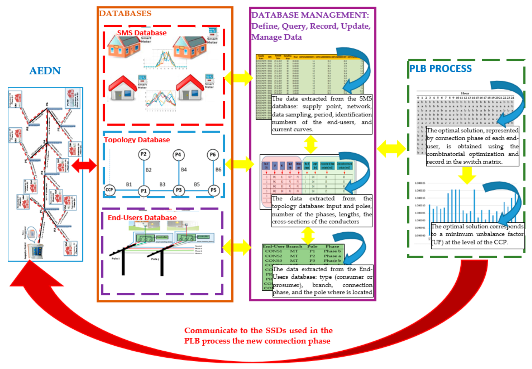
• Implementing a procedure to real-time work for the simultaneous query of three different databases (Topology Database, SMS Database, and End-Users Database) of the DNO for uploading the necessary input data in the PLB process. This procedure allows fast data processing.
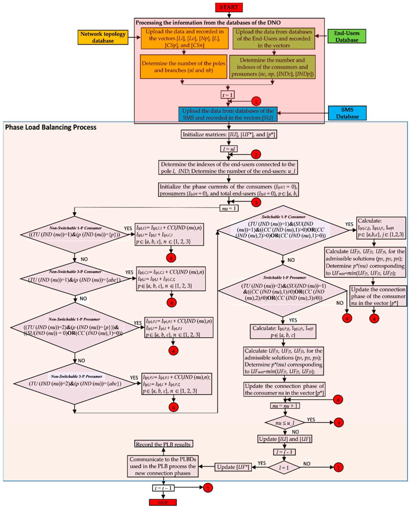
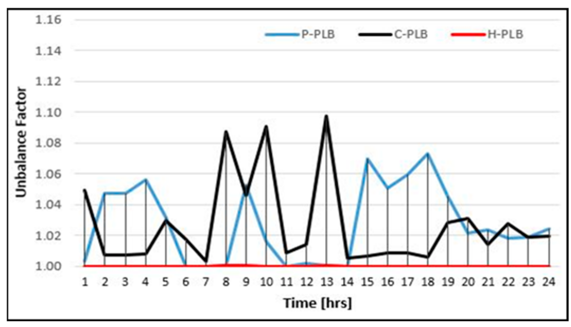
• Proposing an original PLB algorithm applied for other possible PLB cases encountered in the AEDNs: consumer-level (C-PLB), prosumer-level (P-PLB), or hybrid-level (H-PLB) for all 1-P end-users (prosumers and consumers), running regardless of the status of the SSDs (available or unavailable) and the participation degree of the end-users (depending on the absorbed/injected current, equal or different to 0, and the 1-P end-user being considered in the PLB process).
• Conducting a complex study where all possible PLB cases represented by C-PLB, P-PLB, and H-PLB to confirm the accuracy of the proposed methodology, regardless of the structure and participation degree of the end-users.

The methodology can produce meaningful benefits in the AEDNs that integrate a high-speed data communication infrastructure and a master controller in the CCP, having the functions associated with high data acquisition and processing speed.

1.3. Paper Organization

The structure of the paper includes the following sections: Section 2 introduces details regarding each stage from the framework of the proposed methodology; Section 3 presents a complex study performed in a real AEDN from Romania to highlight the accuracy of the methodology in the three possible scenarios (cases) represented by 1-P consumer-level PLB (C-PLB), 1-P prosumer-level PLB (P-PLB), and the hybrid-level (H-PLB); and Section 4 contains the conclusions, also emphasizing future work.

2. Methodology

The proposed methodology allows the coordinated control of the switching devices installed to all 1-P end-users connected to three-phase four-wire AEDN to perform a fast PLB process. It always leads to the best PLB solutions considering the availability or temporary unavailability of the SSDs and the participation degree of the end-users, according to the value of absorbed/injected current (equal or different to 0). Figure 4 presents the flowchart associated with the proposed methodology.

All required information in the PLB process is uploaded from three databases available at the level of the DNO (Topology Database, SMS Database, and End-Users Database). These refer to the topology, identified through the technical and location characteristics of the main elements (poles and conductors) associated with the analysed AEDN, the current profiles of the end-users provided by smart meters identified through the identification numbers, and the end-users regarding the type (consumer or prosumer), the connection phase, and where the pole is located.

The PLB process is based only on the phase swapping of the 1-P consumers and prosumers. For each pole, the optimal local solution, represented by the connection phase of each end-user (consumer/prosumer), is identified with the help of combinatorial optimization. The objective is to minimize the hourly unbalance factor, starting with the end poles and stopping with the EDS, subject to the constraints referring to the phase currents and the number of the end-users connected. Finally, the communication module transmits the new connection phases to the SSDs used in the PLB process. The following paragraphs detail each stage.

2.1. Database Management

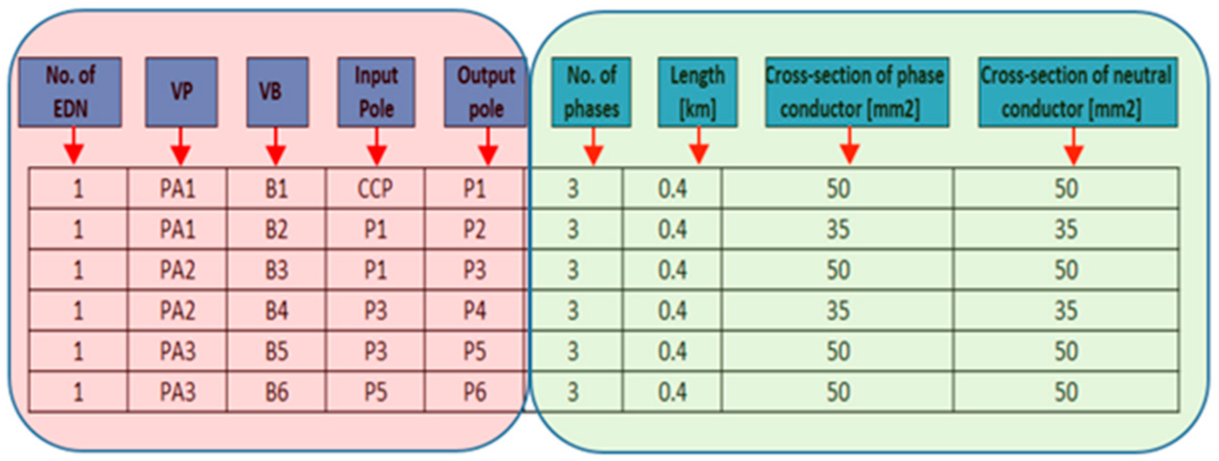
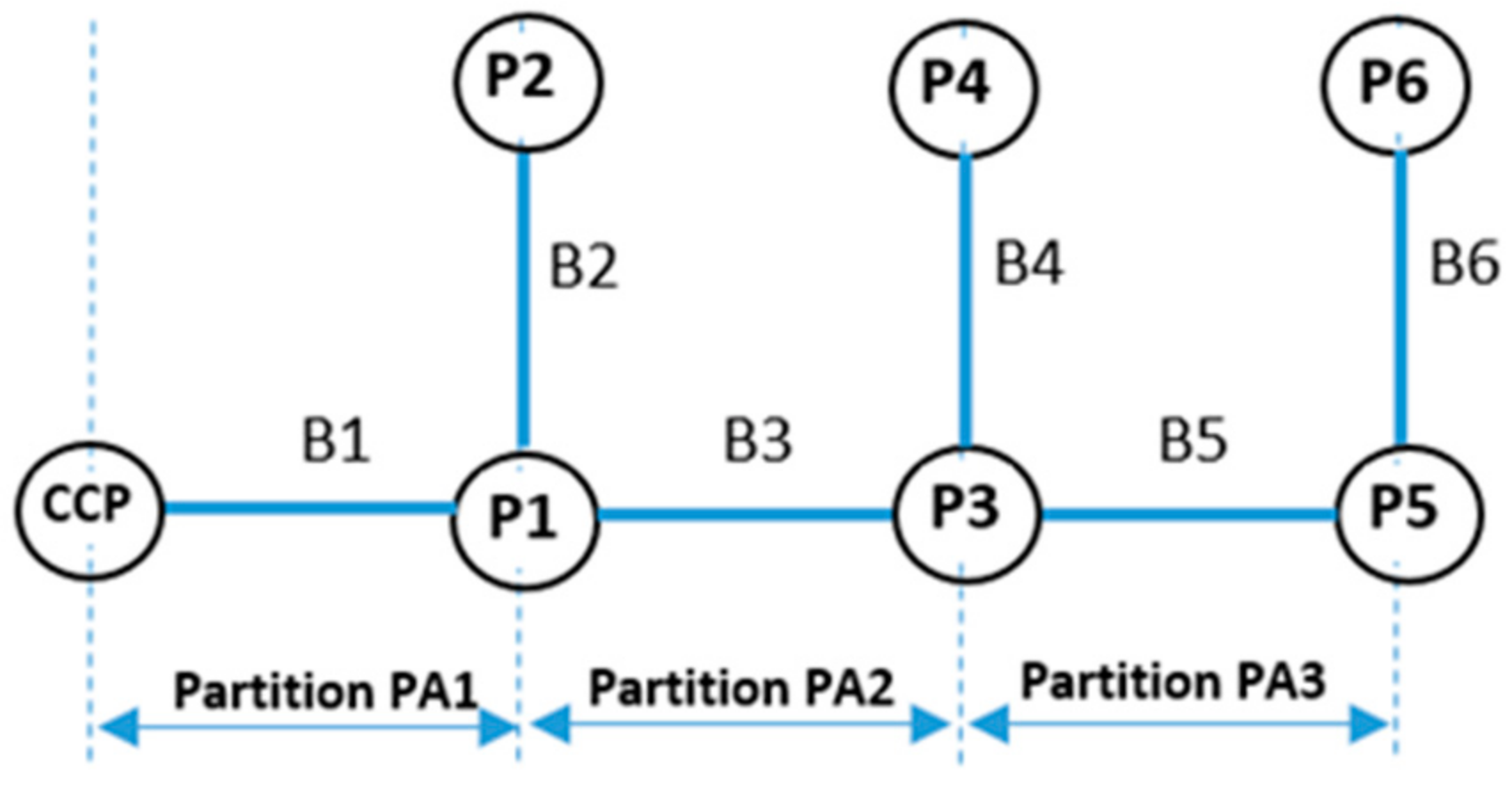
2.1.1. Topology Database

Let there be a radial (tree) AEDN, with Nl poles, nb branches, and a single bus-slack (representing the common coupling point (CCP) with the network operated by the DNO). Under these conditions, nb − Nl + 1 = 0, and accordingly, nb = Nl − 1.

The topology of the AEDN must be recognized quickly, such that the PLB process takes place in real-time. The proposed methodology used the algorithm proposed in [37] based on two vectors which participate in recognizing the topology: the first vector, [VP], having as elements the number of sections from each partition of the AEDN, and a second vector, [VB], containing the name of sections belonging to each partition placed in ascending order. As an example, the topology sequence of the proposed methodology containing details on the recognition process associated with an AEDN with seven poles, including the one on which the EDS is mounted (representing the CCP), and six sections, see Figure 5, based on the vectors [VP] and [VB], to which is added the information from the DNO’s database regarding the length, number of the phases, and the cross-section of the conductors (phase and neutral). Figure 6 contains the topology sequence attached to the AEDN with seven poles.

The elements of the vector [VP] are associated with the partitions PA1, PA2, and PA3. Based on these, the vector [VB] is built, containing the elements B1 and B2 (assigned to partition PA1), B3 and B4 (assigned to partition PA2), and B5 and B6 (assigned to partition PA3). Additionally, the End-Users database is accessed for each AEDN.

The data uploaded from the topology database are stored in the following input vectors used by the PLB algorithm:

[Li]—the input pole of each branch, size (nbx1);

[Lo]—the output pole of each branch, size (nbx1);

[Np]—the number of the phases between each two poles, size (nbx1);

[L]—the length between each two poles, size (nbx1);

[CSp]—the cross-section of the phase conductors between each two poles, size (nbx1);

[CSn]—the cross-section of the neutral conductor between each two poles, size (nbx1).

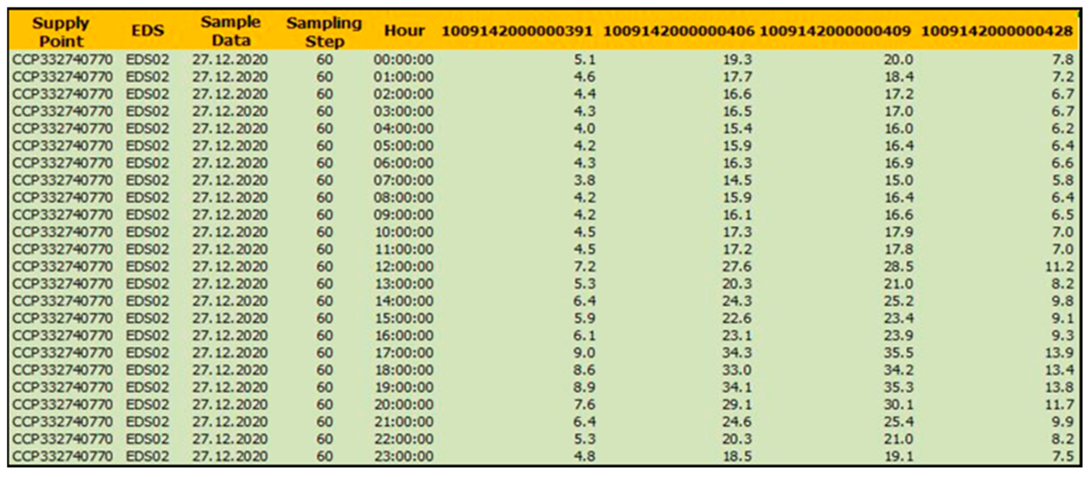
2.1.2. SMS and End-Users Database

The second stage targets establishing the linkage with the database of the DNO attached to the SMS that contains the information regarding the values of the absorbed/injected currents by the consumers and prosumers. Figure 7 presents, as an example, a data sequence uploaded from the SMS database containing the following fields: Supply Point (associated with the identification number of the smart meter installed in the EDS), EDS (the name of the electric distribution substation which supplies the AEDN), Sample Data (the period queried by the decision maker), Sampling Step (15, 30, or 60 min), Hour (the time of data recording), “1009142000000391” (the identification number of the smart meter installed at an end-user).

The signification of each record is described below:

• Supply Point is associated with each EDS through the identification number of the data concentrator having as principal function to collect the data read from the smart meters installed at the end-users allocated to the EDS. This point represents the link with the electric distribution network operated at the medium voltage by the DNO.
• EDS record allows the decision maker to locate the EDS in the network based on its name. Additionally, the information offers the opportunity to identify extremely fast the supplied HV/MV electric substation.
• Sampling Step has a significant influence on data processing. The sampling step of the load curve can be programmable between 5 and 60 min (the normative values being 5, 15, 30, and 60 min). The data sampling of the smart meters installed by the DNOs to the end-users is 60 min in most cases.
• Hour contains the information corresponding to the time with individual hour, minute, and second components (hh:mm:ss) of the recording the value of the load (current or power).
• The next columns record the loads (current or power) transmitted by each smart meter recognized through an identification number in the database (for example, 1009142000000391).

The query considers the filters associated with the Supply Point and Sample Data fields and, depending on Sampling Step (in this case, 60 min), accesses the values of the currents from the smart meters, identified through the identification numbers attached to the analysed AEDN, sending them to the data processing module.

Additionally, the information attached to each end-user regarding the type (consumer or prosumer), the connection phase, and the pole is uploaded from the end-users database using the identification number of the smart meter assigned in the SMS database.

Recording the information for the PLB process is completed in the following vector data structures:

[ID]—the identification number of the smart meter associated with the end-users, size (Nux1);

[SU]—the status of the PLB devices (value 0 (Off) and value 1 (On)), size (Nux1);

[CC]—the hourly phase currents of the end-users, size (Nux1);

[TU]—the type of the end-users (1—consumers and 2—prosumers), size (Nux1);

[p]—the connection phases of the end-users (a, b, and c, for the 1-P end-users, and abc, for the 3-P end-users), size (Nux1);

[Nl]—the poles where are assigned the end-users, size (Nux1);

Within the above, nb is the number of the branches from the AEDN, and Nu signifies the number of the end-users (consumers and prosumers).

2.2. The PLB Mathematical Model

The proposed PLB algorithm can be used only for the phase swapping of the 1-P consumers and prosumers connected to a radial AEDN. It aims to minimize the hourly unbalance factor (UF) at the level of each pole, starting with the end poles and stopping with the EDS, subject to the constraints referring to the phase currents and the number of the end-users connected. The necessary data used in the PLB process are extracted from the input vectors, and their significance inside the algorithm is the following:

P, prosumer; C, consumer; U, end-user;

T, the analysed time interval (in our case study, T = 24 h);

p, the connection phase of the end-users to the AEDN, p ∈ {a, b, c};

n_p—the number of the phases (in the AEDNs with four-wires, n_p = 3);

N_l, the number of the poles from the AEDN, also including the pole where the electric distribution substation (EDS) is mounted;

N_C,_l the number of the consumers connected to the pole l, l ∈{1, …, N_l};

N_P,l, the number of the prosumers connected to pole l, l ∈{1, …, N_l};

N_U,l, the total number of the end-users (prosumers and consumers) connected to pole l, l ∈{1, …, N_l};

I^(t)_{p},l, the phase currents absorbed/injected by the end-users U_l, U_l ∈ {1,…, N_U,l} at the level of the pole l, l ∈{1, …, N_l}, at the hour t, t ∈ {1,…,T};

I^(t)_m,l, the mean, m, of the phase currents absorbed/injected by the end-users U_l, U_l ∈ {1,…, N_U,l} at the level of the pole l, l ∈{1, …, N_l}, at the hour t, t ∈ {1,…,T};

I^(t)_{p},C,l, the phase currents absorbed by the consumers C_l, C ∈ {1,…, N_C,l}, connected to the pole l, l ∈{1, …, N_l}, at the hour t, t ∈ {1,…,T};

I^(t)_{p},P,l, the phase currents injected/absorbed by the prosumers P_l, P_l ∈ {1,…, N_P,l}, connected to pole l, l ∈{1, …, N_l}, at the hour t, t = 1,…,T;

I^(t)_{p},P,(l+1), the phase currents aggregated at the pole (l+1) downstream by the pole l, l ∈{1, …, N_l}, at the hour t, t = 1,…,T (for the end poles the value is 0).

The variables α^(t)_{p},l, having the value 1 or 0, have been defined to determine if the 1-P end-user (prosumer or consumer) is or is not connected on the phase p, at the hour t.

The objective function has the expression,

$$\min (U{F}_l^{(t)})=\min \left(\frac{{\displaystyle \sum _{p\in \{a,b,c\}}{\left(\frac{I_{\left\{p\right\},l}^{(t)}}{I_{m,l}^{(t)}}\right)}^2}}{n_p}\right)(\forall )t\in \{1,\dots ,T\},(\forall )l\in \{1,\dots ,N_l\}$$

(1)

where

$$I_{m,l}^{(t)}=\frac{{\displaystyle \sum _{p\in \{a,b,c\}}{I}_{\left\{p\right\},l}^{(t)}}}{n_p}(\forall )t\in \{1,\dots ,T\},(\forall )l\in \{1,\dots ,N_l\}$$

(2)

Additionally, the constraints referring to the phase currents and the number of the end-users connected are the following:

$$I_{\left\{p\right\},l}^{(t)}=I_{\left\{p\right\},C,l}^{(t)}+I_{\left\{p\right\},P,l}^{(t)}+I_{\left\{p\right\},(l-1)}^{(t)},(\forall )t\in \{1,\dots ,T\},(\forall )l\in \{1,\dots ,N_l\},p\in \{a,b,c\}$$

(3)

$$I_{\left\{p\right\},C,l}^{(t)}={\displaystyle \sum _{i=1}^{N_{\left\{p\right\},C,l}^{(t)}}{\alpha }_{\left\{p\right\},l,i}^{(t)}\cdot }{I}_{C,l,i}^{(t)},(\forall )t\in \{1,\dots ,T\},(\forall )l\in \{1,\dots ,N_l\},p\in \{a,b,c\}$$

(4)

$$I_{\left\{p\right\},P,l}^{(t)}={\displaystyle \sum _{j=1}^{N_{\left\{p\right\},P,l}^{(t)}}{\alpha }_{\left\{p\right\}.l,j}^{(t)}\cdot }{I}_{P,l,j}^{(t)},(\forall )t\in \{1,\dots ,T\},(\forall )l\in \{1,\dots ,N_l\},p\in \{a,b,c\}$$

(5)

$$N_{C,l}={\displaystyle \sum _{p\in \{a,b,c\}}{N}_{\left\{p\right\},C,l}^{(t)},}(\forall )t\in \{1,\dots ,T\},(\forall )l\in \{1,\dots ,N_l\}$$

(6)

$$N_{P,l}={\displaystyle \sum _{p\in \{a,b,c\}}{N}_{\left\{p\right\},P,l}^{(t)},}(\forall )t\in \{1,\dots ,T\},(\forall )l\in \{1,\dots ,N_l\}$$

(7)

$$N_{U,l}=N_{C,l}+N_{P,l},(\forall )l\in \{1,\dots ,N_l\}$$

(8)

The decision variables for the optimization process are represented by the variables α^(t)_{p},l, which can have the values 1 or 0, indicating if the 1-P end-users can or cannot connect to a phase. The minimization of the hourly unbalance factor (UF) at the level of each pole (also including the EDS) represents the aim of the optimization process subject to the constraints referring to the phase currents and the end-users connected, see relation 1. Thus, the balance of the phase currents at the level of each pole l, l ∈ {1, …, Nl}, from the AEDN at the hour t, t ∈ {1, …, T}, must be fulfilled such that the currents of the prosumers, I^(t)_{p},P,l, the consumers, I^(t)_{p},C,l, and the current flow downstream by the pole l must be equal with the current flow upstream by the pole l, I^(t)_{p},P,(l+1), see relation 3. Additionally, the current of consumers on each phase, I^(t)_{p},C,l, must be equal with the sum of the currents absorbed by the consumers connected on the phase based on the decision making represented by the variable α^(t)_{p},l, see relation 4. The same constraint has applied the prosumers, see relation 5. Regarding the end-users connected, the total number of the consumers on the three phases, p ∈ {a, b, c}, at each pole l, l ∈ {1, …, N_l}, at the hour t, t ∈ {1, …, T}, must be equal with the one identified in the database, N_C,l, see relation 6. A similar constrain has been imposed on the prosumers, where the total number of the prosumers connected on the three phases, p ∈ {a, b, c}, at each pole l, l ∈ {1, …, N_l}, at the hour t, t ∈ {1, …, T}, must be equal with the one identified in the database, N_P,l, see relation 7. Finally, the number of prosumers and consumers must be the same as the total number of end-users connected at each pole l, l ∈ {1, …, N_l}, see relation 8.

For a pole l, l = {1, …, N_l}, the optimal local solution [p*], represented by connection phase of each end-user (consumer/prosumer), is obtained using the combinatorial optimization [38]. Formally, a combinatorial optimization problem associated with the PLB process refers to a set of possibilities to which the objective given by the relation (1) is associated. An embodiment of the PLB problem is the pair (A, UF) in which A is a finite set and UF: A → ℤ is some function. The aim is to identify a solution [p*] included in set A that minimizes the UF at the level of the EDS. Thus, the elements of set A represent admissible solution UF is the objective function, and [p*] is the optimal solution of the PLB problem. The set A includes a small number of the elements (only three combinations associated with each end-user), and as such, the optimal solution results from listing all these solutions. The complete enumeration operation has been used to determine the optimal solution considering that the number of the admissible solutions is small, as can be seen in

Table 2. The admissible solutions associated with the phase swapping of the consumer/prosumers.

Consumer/Prosumer Type	Initial Positions	Final Positions
1-P type	a b c	b/c/a c/a/b a/b/c

.

Table 3. The implementation procedure of the proposed PLB methodology.

Stage 1. Identifying the topology of the AEDN

Upload the data from the topology database and recorded in the vectors [L], [CS], [Np], [Li], and [Lo]. → Determine from the vector [Li] the number of the poles: nl = length(Li)+1; → Determine from the vector [Li] the number of the branches: nb = length(Li).

Stage 2. Identifying the topology of the AEDN Querying the databases of the DNO (SMS and End-Users)

Upload the data from databases of End-Users and recorded in the vectors [Nl], [p], [ID], and [TU]. → Determine from the vector [TU] the following information: − the indexes of the consumers: INDc = find([TU] = 1); − the number of the consumers: nc = length([INDc]); − the indexes of the prosumers: INDp = find(TU = 2); − the number of the prosumers: np = length(INDp); for each hour t = 1: T → Upload the data from databases of the SMS and recorded in the vectors [SU] and [CC].

Stage 3. The PLB process implemented to the level of each pole:

→ Initialization of the matrix corresponding to the total phase currents of the end-users connected at each pole, [IU], having the size (nlx3), the vectors referring to the unbalance factor at the level of the EDS, [UF*], and the optimal connection phase of the end-users, [p*], with the size (Tx1). → Set the index of the pole (starting with the end poles, in descending order): l = nl; → while(l ≥ 1) and (l ≤ nl); − Determine the indexes of the end-users connected to the pole l: IND = find ([Nl] = l); − Determine the number of the end-users: u_l = length ([IND]); − Initialize the total phase currents corresponding to: consumers: IaCl = 0, IbCl = 0, IcCl = 0; prosumers: IaPl = 0, IbPl = 0, IcPl = 0; end-users: Ial = 0, Ibl = 0, Icl = 0; − Set index of the end-users: nu = 0; − while nu≤ u_l Increase index of the end-users: nu = nu+1; case Non-Switchable 1-P Consumer (the end-user nu is a consumer having the SSD with the status Off or the hourly absorbed phase current with the null value).     • if ((TU (IND (nu)) = 1) AND (p (IND (nu)) = {a})) AND ((SU(IND (nu)) = 0) OR (CC (IND (nu),1) = 0));            Update the total current of the consumers on the phase a: IaCl = IaCl + CC (IND (nu),1);            Calculate the total current on the phase a: Ial = Ial + IaCl;     • if ((TU (IND (nu)) = 1) AND (p (IND (nu)) = {b})) AND ((SU(IND (nu)) = 0) OR (CC (IND (nu), 2) = 0));         Update the total current of the consumers on the phase b: IbCl = IbCl + CC (IND (nu),2);         Calculate the total current on the phase b: Ibl = Ibl + IbCl;     • if ((TU (IND (nu)) = 1) AND (p (IND (nu)) = {c})) AND ((SU(IND (nu)) = 0) OR (CC (IND (nu), 3) = 0));         Update the total current of the consumers on the phase c: IcCl = IcCl + CC (IND (nu),3);         Calculate the total current on the phase c: Icl = Icl + IcCl; case Non-Switchable 3-P Consumer (the end-user nu is a 3-P consumer).     • if (TU (IND (nu)) = 1) AND (p (IND (nu)) = {abc}):         Update the total current of the consumers on all phases:         IaCl = IaCl + CC (IND (nu),1); IbCl = IbCl + CC (IND (nu),2); IcCl = IcCl + CC (IND (nu),3).         Calculate the total current on all phases:         Ial = Ial + IaCl; Ibl = Ibl + IbCl; Icl = Icl + IcCl. case Non-Switchable 1-P Prosumer (the end-user nu is a prosumer having the SSD with the status Off or the hourly injected/absorbed phase current with the null value).∙     • if ((TU (IND (nu)) = 2) AND (p (IND (nu)) = {a})) AND ((SU(IND (nu)) = 0) OR (CC (IND (nu),1) = 0));         Update the total current of the prosumers on the phase a: IaPl = IaPl + CC (IND (nu),1);         Calculate the total current on the phase a: Ial = Ial + IaPl;     • if ((TU (IND (nu)) = 2) AND (p (IND (nu)) = {b})) AND ((SU(IND (nu)) = 0) OR (CC (IND (nu), 2) = 0));            Update the total current of the prosumers on the phase b: IbPl = IbPl + CC (IND (nu),2);            Calculate the total current on the phase b: Ibl = Ibl + IbPl;     • if ((TU (IND (nu)) = 2) AND (p (IND (nu)) = {c})) AND ((SU(IND (nu)) = 0) OR (CC (IND (nu), 3) = 0));            Update the total current of the prosumers on the phase c: IcPl = IcPl + CC (IND (nu),3);            Calculate the total current on the phase c: Icl = Icl + IcPl. case Non-Switchable 3-P Prosumer (the end-user nu is a 3-P prosumer).     • if (TU (IND (nu)) = 2) AND (p (IND (nu)) = {abc})         Update the total current of the prosumers on all phases:         IaPl = IaPl + CC (IND (nu),1); IbPl = IbPl + CC (IND (nu),2); IcPl = IcPl + CC (IND (nu),3).         Calculate the total current on all phases:           Ial = Ial + IaPl; Ibl = Ibl + IbPl; Icl = Icl + IcPl. case Switchable 1-P Consumer (the end-user nu is a consumer having the SSD with the status On and the hourly absorbed phase current with the positive value).     • if (TU (IND (nu)) = 1) AND (SU(IND (nu)) = 1) AND ((CC (IND (nu),1) > 0) OR (CC (IND (nu),2) > 0)         OR (CC (IND (nu),1) > 0));      Identification of the optimal connection solution of the consumer nu using the combinatorial optimization:          Admissible solution 1–connection on the phase a           Determine the feasible phase currents: IaCf1 = IaCl + CC (IND (nu),1); IbCf1 = IbCl; IcCf1 = IcCl;           Determine the feasible total phase currents: Ialf1 = Ial + IaCf1; Iblf1 = Ibl+ IbCf1; Iclf1 = Icl+ IcCf1;           Determine the mean of the phase currents, Imlf1 (formula (2));           Determine the UFf1 (formula (1)).          Admissible solution 2–connection on the phase b              Determine the feasible phase currents: IaCf2 = IaCl; IbCf2 = Ibcl + CC (IND (nu), 2); IcCf2 = IcCl;              Determine the feasible total phase currents: Ialf2 = Ial + IaCf2; Iblf2 = Ibl+ IbCf2; Iclf2 = Icl+ IcCf2;              Determine the mean of the phase currents, Imlf2 (formula (2));              Determine the UFf2 (formula (1)).          Admissible solution 3–connection on the phase c              Determine the feasible phase currents: IaCf3 = IaCl; IbCf3 = IbCl; Iccf3 = IcCl + CC (IND (nu), 3);              Determine the feasible total phase currents: Ialf3 = Ial + IaCf3; Iblf3 = Ibl+ IbCf3; Iclf3 = Icl+ IcCf3;              Determine the mean of the phase currents, Imlf3 (formula (2));              Determine the UFf3 (formula (1)).          Calculate the optimal solution that leads to the minimization of the UF: UFmin = min (UFf1, UFf2, UFf3);              if Optimal solution = Admissible solution 1              Update the vector [p*]: p* (IND (nu)) = {a};              Update the total phase currents of consumers: IaCl = IaCf1; IbCl = IbCf1; IcCl = IcCf1;              Update the total phase currents of the end-users: Ial = Ialf1; Ibl = Iblf1; Icl = Iclf1.              if Optimal solution = Admissible solution 2           Update the vector [p*]: p* (IND (nu)) = {b};           Update the total phase currents of consumers: IaCl = IaCf2; IbCl = IbCf2; IcCl = IcCf2;           Update the total phase currents of the end-users: Ial = Ialf2; Ibl = Iblf2; Icl = Iclf2.              if Optimal solution = Admissible solution 2           Update the vector [p*]: p* (IND (nu)) = {c};           Update the total phase currents of prosumers: IaCl = IaCf3; IbCl = IbC3; IcCl = IcCf3;           Update the total phase currents of the end-users: Ial = Ialf3; Ibl = Iblf3; Icl = Iclf3. case Switchable 1-P Prosumer (the end-user nu is a prosumer having the SSD with the status On and the hourly absorbed/injected phase current with the different value by 0).     • if (TU (IND (nu)) = 2) AND (SU(IND (nu)) = 1) AND ((CC (IND (nu),1) ≠ 0) OR (CC (IND (nu),2) ≠0) OR         (CC (IND (nu),3) ≠0)).        Identification of the optimal connection solution of the prosumer nu using the combinatorial optimization:           Admissible solution 1–connection on the phase a         Determine the feasible phase currents: IaPf1 = IaPl + CC (IND (nu),1); IbPf1 = IbPl; IcPf1 = IcPl;         Determine the feasible total phase currents: Ialf1 = Ial + IaPf1; Iblf1 = Ibl+ IbPf1; Iclf1 = Icl+ IcPf1;         Determine the mean of the phase currents, Imlf1 (formula (2));         Determine the UFf1 (formula (1)).         Admissible solution 2–connection on the phase b           Determine the feasible phase currents: IaPf2 = IaPl; IbPf2 = IbPl + CC (IND (nu), 2); IcPf2 = IcPl;           Determine the feasible total phase currents: Ialf2 = Ial + IaPf2; Iblf2 = Ibl+ IbPf2; Iclf2 = Icl+ IcPf2;           Determine the mean of the phase currents, Imlf2 (formula (2));           Determine the UFf2 (formula (1)).        Admissible solution 3–connection on the phase c            Determine the feasible phase currents: IaPf3 = IaPl; IbPf3 = IbPl; IcPf3 = IcPl + CC (IND (nu), 3);            Determine the feasible total phase currents: Ialf3 = Ial + IaPf3; Iblf3 = Ibl+ IbPf3; Iclf3 = Icl+ IcPf3;       Determine the mean of the phase currents, Imlf3 (formula (2));            Determine the UFf3 (formula (1)).         Calculate the optimal solution that leads to the minimization of the UF: UFmin = min (UFf1, UFf2, UFf3);            if Optimal solution = Admissible solution 1             Update the vector [p*]: p* (IND (nu)) = {a};             Update the total phase currents of prosumers: IaPl = IaPf1; IbPl = Ibpf1; IcPl = IcPf1;             Update the total phase currents of the end-users: Ial = Ialf1; Ibl = Iblf1; Icl = Iclf1.            if Optimal solution = Admissible solution 2         Update the vector [p*]: p* (IND (nu)) = {b};         Update the total phase currents of prosumers: IaPl = IaPf2; IbPl = IbPf2; IcPl = IcPf2;         Update the total phase currents of the end-users: Ial = Ialf2; Ibl = Iblf2; Icl = Iclf2.            if Optimal solution = Admissible solution 3         Update the vector [p*]: p* (IND (nu)) = {c};         Update the total phase currents of prosumers: IaPl = IaPf3; IbPl = IbPf3; IcPl = IcPf3;         Update the total phase currents of the end-users: Ial = Ialf3; Ibl = Iblf3; Icl = Iclf3.     • Update the matrix [IU]: IU (l, 1) = Ial, IU (l, 2) = Ibl, and IU (l, 3) = Icl;     • Update the vector [UF]: UF(l) = UFmin;   − Decrease index of the pole: l = l − 1; → Update the vector [UF*]: UF*(t) = UF(1); → Communicate to the PLBDs used in the PLB process the new connection phases; → Record the PLB results in matrix [PA]; Increase the index of hour: t = t + 1; Print the results.

details the stages of the implementation procedure, and Figure 8 presents the flowchart of the proposed centralized control methodology.

The procedure can be used for all strategies applied in an AEDN: 1-P consumer-level (C-PLB), 1-P prosumer-level (P-PLB), and hybrid-level (H-PLB) for all 1-P end-users (prosumers and consumers). Additionally, the procedure runs regardless of the status of the SSDs (On/Off) and the absorbed/injected current (equal/different to 0), the 1-P end-user (prosumer or consumer) being considered in the PLB process or not.

As the 3-P prosumers and consumers can be also connected to the AEDNs, the algorithm must consider their presence and, accordingly, are treated as non-switchable 1-P prosumers/consumers, without affecting the PLB process. Regarding the 3-P prosumers, they should be equipped with special complex devices based on tracking the values of phase currents and modifying the injection for balancing at the level of the pole or area.

Regarding the resiliency of the proposed coordinated control system, we referred to a clear definition from [39], formulated by Shan et al., “resiliency is defined as the ability to rebound quickly to the original state given an interruption in the electric power grid”. The proposed system can carry out its task in the face of adversity, providing required capabilities despite excessive switching operations that can cause disruptions at some end-users or various phase outages due to the faults in the AEDN.

3. Case Study

The proposed methodology has been tested on a LV AEDN belonging to a Romanian DNO with 114 end-users integrated into the Smart Metering System (SMS), including 104 consumers (103 single-phase/1 three-phase) and 10 single-phase prosumers, during a day when the peak load has been recorded. The prosumers have PV panels with the installed power of 1.5, 3, and 5 kW, without storage systems. The common coupling point (CCP) with the network operated by the DNO is on the low voltage busbar (0.4 kV) of the electric distribution substation.

Figure 9 presents the topology of the AEDN, and details of the technical characteristics can be seen in the Supplementary File Additional Data of the Topology.

Table 4. The topology data associated with the analysed AEDN.

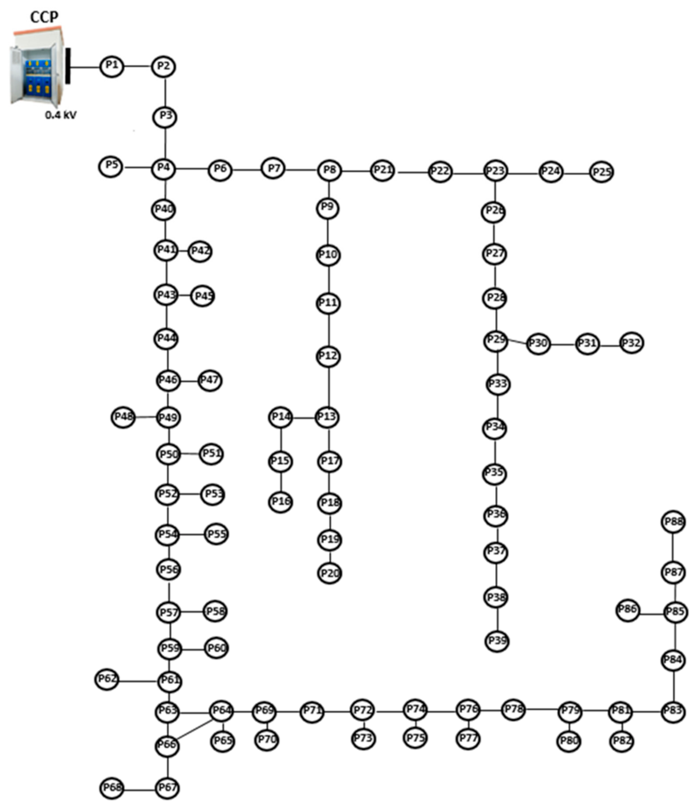
AEDN	Number of Poles	Pole i	Pole j	Length (km)	Cross-Section (mm2)		Consumers/ Prosumers
					Phase	Neutral
Main trunk (MT)	53	CCP	P5	0.20	3 × 50	50	5
		P5	P66	1.08	3 × 50	50	28/7
		P66	P88	0.80	3 × 50	50	19/1
		P66	P68	0.08	1 × 16	25	1
Lateral branch (LB)	35	P5	P13	0.32	3 × 35	35	11
		P13	P20	0.28	1 × 35	35	6
		P8	P32	0.48	3 × 35	35	22/2
		P29	P39	0.28	1 × 25	25	12

synthesizes the information on the number of consumers/prosumers, the length, and cross-sections of the main trunk (MT)/lateral branch (LB).

The AEDN has a main trunk characterized by a total length of 2.16 km, containing 53 poles to which 61 end-users (53 consumers/8 prosumers) are connected. A single lateral branch leaves from the pole P5 having 1.36 km and 53 end-users (51 consumers/2 prosumers) connected at 35 poles. Additionally, the wires of the main trunk have a cross-section of 50 mm², unlike the lateral branch with a cross-section of 35 mm². An uneven allocation of the end-users was observed both on the main trunk and the lateral branch, see

Table 5. Location and connected phase (initial situation) of the end-users in the AEDN.

End-User	Branch	Pole	Phase	End-User	Branch	Pole	Phase	End-User	Branch	Pole	Phase
CONS1	MT	P1	Phase b	CONS83	MT	P63	Phase b	CONS21	LB	P20	Phase c
CONS2	MT	P2	Phase a	CONS84	MT	P65	Phase b	CONS22	LB	P20	Phase c
CONS3	MT	P3	Phase b	CONS85	MT	P68	Phase b	CONS23	LB	P21	Phase b
CONS4	MT	P4	Phase b	CONS86	MT	P70	Phase b	CONS24	LB	P21	Phase c
CONS5	MT	P5	Phase b	CONS87	MT	P71	Phase a	CONS25	LB	P22	Phase c
PROS3	MT	P40	Phase b	CONS88	MT	P71	Phase b	CONS26	LB	P22	Phase c
PROS4	MT	P40	Phase b	CONS89	MT	P71	Phase b	CONS27	LB	P23	Phase c
CONS57	MT	P41	Phase a	CONS90	MT	P71	Phase b	CONS28	LB	P23	Phase c
CONS58	MT	P41	Phase b	CONS91	MT	P72	Phase b	CONS29	LB	P24	Phase c
CONS59	MT	P41	Phase b	CONS92	MT	P73	Phase b	CONS30	LB	P25	Phase c
CONS60	MT	P42	Phase b	CONS93	MT	P75	Phase b	CONS31	LB	P26	Phase c
CONS61	MT	P42	Phase b	CONS94	MT	P75	Phase b	CONS32	LB	P26	Phase c
CONS62	MT	P43	Phase c	CONS95	MT	P76	Phase a	CONS33	LB	P26	Phase c
CONS63	MT	P45	Phase b	CONS96	MT	P77	Phase b	CONS34	LB	P26	Phase c
PROS5	MT	P45	Phase b	CONS97	MT	P80	Phase b	CONS35	LB	P27	Phase c
CONS64	MT	P46	Phase b	CONS98	MT	P80	Phase b	CONS36	LB	P27	Phase c
CONS65	MT	P47	Phase b	PROS10	MT	P81	Phase b	CONS37	LB	P27	Phase a
CONS66	MT	P47	Phase b	CONS99	MT	P82	Phase b	CONS38	LB	P28	Phase a
CONS67	MT	P47	Phase b	CONS100	MT	P82	Phase b	CONS39	LB	P28	Phase c
PROS6	MT	P47	Phase b	CONS101	MT	P85	Phase b	CONS40	LB	P28	Phase c
PROS7	MT	P47	Phase b	CONS012	MT	P86	Phase b	CONS41	LB	P30	Phase c
CONS68	MT	P48	Phase b	CONS103	MT	P86	Phase b	PROS1	LB	P30	Phase a
PROS8	MT	P51	Phase a	CONS104	MT	P88	Phase b	PROS2	LB	P30	Phase c
CONS69	MT	P52	Phase b	CONS6	LB	P6	Phase b	CONS42	LB	P31	Phase c
CONS70	MT	P52	Phase b	CONS7	LB	P6	Phase c	CONS43	LB	P32	Phase c
CONS71	MT	P53	Phase b	CONS8	LB	P7	Phase c	CONS44	LB	P32	Phase c
CONS72	MT	P55	Phase c	CONS9	LB	P8	Phase b	CONS45	LB	P33	Phase c
CONS73	MT	P56	Phase a	CONS10	LB	P9	Phase c	CONS46	LB	P33	Phase c
CONS74	MT	P58	Phase b	CONS11	LB	P10	Phase abc	CONS47	LB	P34	Phase c
CONS75	MT	P59	Phase a	CONS12	LB	P11	Phase c	CONS48	LB	P35	Phase c
CONS76	MT	P59	Phase b	CONS13	LB	P11	Phase c	CONS49	LB	P36	Phase c
PROS9	MT	P59	Phase b	CONS14	LB	P12	Phase a	CONS50	LB	P36	Phase c
CONS77	MT	P60	Phase b	CONS15	LB	P13	Phase a	CONS51	LB	P37	Phase c
CONS78	MT	P60	Phase b	CONS16	LB	P13	Phase a	CONS52	LB	P37	Phase b
CONS79	MT	P61	Phase b	CONS17	LB	P16	Phase a	CONS53	LB	P38	Phase c
CONS80	MT	P61	Phase b	CONS18	LB	P16	Phase a	CONS54	LB	P38	Phase c
CONS81	MT	P62	Phase a	CONS19	LB	P19	Phase c	CONS55	LB	P38	Phase c
CONS82	MT	P62	Phase b	CONS20	LB	P19	Phase c	CONS56	LB	P39	Phase c

MT—Main trunk; LB—Lateral Branch; CONS—consumer; and PROS—prosumer.

and Figure 10. Most of the end-users connected at the poles from the main trunk are connected on phase b (83.6%) and a smaller number on phases a (13.1%) and c (3.3%). The lateral branch has a similar situation, with a high allocation on phase c (75.5%) and a discrete presence on phases a (15.1%) and b (7.5%). Only one three-phase end-user (1.9%) from the consumers’ category, connected on the lateral branch, has been identified in the AEDN.

The proposed methodology has been tested in this AEDN to demonstrate efficiency for the most complex topologies. The average length of an EDN is by 1.2 km, having 30 poles, to which about 60 consumers are connected [40,41]. The topology data associated with the analysed AEDN (total length, number of the poles, and end-users) far exceed these average values.

All data were recorded in the input vectors having the size (1x Nc), where Nc represents the number of the end-users: [P] (number of the pole), [p] (allocated phase), [L] (length of each section), [Ct] (conductor type, single-phase or three-phase), [CSp] (cross-section of the phase conductor), and [CSn] (cross-section of the neutral conductor). The elements of the vectors [L], [Ct], [CSp], and [CSn] refer to the information of the section between two poles of the main trunk or lateral branch. Additionally, the vectors allow the decision maker to know the detailed topology of the analysed AEDN.

Additional data referring to the hourly current of the consumers and the injected/absorbed current of the prosumers are known in real-time. The processing module queried the SMS’ database and uploaded the recorded values of each end-user from the analysed AEDN in the vectors [IC], for the consumers, and [IP], for the prosumers. The current profiles are available in the Supplementary File End-Users’ Current Profiles.

After uploading the data, the next step has been initialized to obtain the aggregate value of the phase powers at the CCP level and calculate the unbalance factor. Figure 11 and Figure 12 show the hourly values of the aggregated phase currents and the UF at the CCP level in the initial case, without PLB (W-PLB). Inverse current flows from AEDN to CCP on phases a and b, at hours H9 and H10, respectively, and phase a at hour H13, have been recorded, which means that prosumers have higher current injections than the demands of consumers connected on these phases. Additionally, high differences between the phase currents recorded at each hour, leading to values of the UF at every hour over the target accepted by the DNO (UF = 1.1, corresponding to a degree of current unbalance of 10%), represented in red in the figure. The maximum values of the UF have been recorded at the hours H8 and H13 (1.87 and 1.86), and the average value reached 1.30.

In these conditions, the steps to establish a phase load balancing in the analysed AEDN, having as objective obtaining the hourly UFs below the target value imposed by the DNO (1.1) at the CCP level, have been completed. The poles located at the end of the network represent the points where the algorithm initialized, and the last point corresponds to the CCP, where the UF must have the minimum value subject to the constraints (2)–(8). The aggregation of the injected/absorbed currents is investigated in each point, identified through a pole, and the locally optimal solution corresponds to the combination associated with the phase allocations of the end-users that leads to the minimum value of the UF. Each solution is recorded in the matrix [PA] on the column assigned to the hour when the PLB process is ongoing and the row corresponding to each end-user allocated to the pole. All elements associated with matrix [PA] are available in the Supplementary File Switching Operation Matrix. Figure 13 presents the switching operations of the SSDs installed to the end-users in the analysed period (24 h).

The analysis of the optimal solutions associated with the connection phase at each hour and recorded in the matrix [PA], revealed that each SSD installed at the end-users connected at the poles on the main trunk had, on average, 13 switching operations (Figure 13a), and 16 for each SSD on the lateral branch (Figure 13b), highlighted with the red line.

From all consumers, the maximum number of switching operations (20) has been performed by CONS35 (pole P27, on the lateral branch). The prosumers PROS1 (pole P30), on the lateral branch, PROS3 (pole P40), PROS4 (pole P40), and PROS 7 (pole P47) on the main trunk had the maximum number of the switching operations (16). These switching operations can be easily supported due to the high reliability associated with the components of the SSDs.

The number of end-users who participated in the PLB process at each hour was different. The maximum number has been recorded at the hour H16 (90 end-users) and the minimum at the hour H3 (31 end-users). The participation degree at the PLB process was an average of 60% (68 end-users) per hour, see Figure 14 (red line).

Figure 15 presents the value of the objective function represented by the minimum value of the UF at the CCP level on the LV side. The average value of the UF is 1.000043. In the following, the value of UF will be considered equal with 1.00 in the H-PLB case.

The highest values of the UF belong to the hours H8, H9, and H13 (same hours as in the unbalance case), but these are smaller, close by 1.00 (the ideal values). Compared with the unbalance case, the phase currents at the level of the CCP are very close, and there are no inverse current flows from the AEDN to the CCP (see Figure 16). Additionally, the absorbed phase currents from the CCP at the hour H9 have the smallest values, close to 0, with a balance of the injected/absorbed currents in the network.

The algorithm has been implemented in Matlab2016, the time computing obtained for the optimal solution was 1.13 s corresponding to 24 h. The performance is better than that obtained with the heuristic algorithm based on the phase swapping at the pole level (HA-PSPL) [15], the genetic algorithm based on the phase swapping at the substation level (AG-PSSL) [42], and particle swarm optimization algorithm based on the phase swapping at the substation level (PSO-PSSL) [43], where an EDN having the same topology has been used (see

Table 6. The performance of the PLB algorithms based computational times.

No.	PLB Algorithms	Computational Times [Seconds]
1	H-PLBA (Proposed)	1.13
2	HA-PSPL [15]	1.26
4	AG-PSSL [42]	291
3	PSO-PSSL [43]	348

). The same technical characteristics have been considered for the computer (Intel Core i7 processor, 3.10 GHz, 4GB RAM) to perform this comparison.

The other two PLB cases (frequently encountered in the EDNs), applied to the consumer-level (PLB-C) and prosumer-level (PLB-P), have been analysed and compared with the H-PLB case, see Figure 17. An analysis of the results led to the following observations regarding the hourly values of the UF. In the P-PLB procedure, two-time intervals, H1–H5 and H15–H24, have been identified, where the UF had the higher average values (1.037 and 1.04, respectively). Additionally, a small average value of 1.008 has been obtained in the time interval H6–H14. In the C-PLB procedure, the results were the opposite. The UF had the higher values in the time interval H6–H14 (1.041) and smaller values (1.02 and 1.017) in the other two intervals (H1–H5 and H15–H24).

Figure 18 shows the average value of the UF in the three analysed PLB cases. The P-PLB and C-PLB cases recorded similar values of the UF (1.028 vs. 1.027), which were higher than in the H-PLB. However, they were below 1.1 (target imposed by the DNO) with approximately 0.07, emphasizing the effectiveness of the proposed PLB algorithm in these two extreme cases. These positive effects were reflected on the values of the phase currents at the level of the CCP.

Figure 19 and Figure 20 detail the results where the time intervals above highlighted can be better observed. There is still an inverse current flow in all phases at the hour H10 in the P-PLB case, but the values are smaller than in the unbalanced case (W-PLB). These current flows did not record in the C-PLB case due to the high number of combinations associated with the consumers. The optimal solutions, characterized through a balance between the injected/absorbed currents by the prosumers and consumers, led to the small phase load unbalances in the C-PLB case.

Table 7. The hourly phase currents and the unbalance factor calculated for all analysed cases *, in (kW).

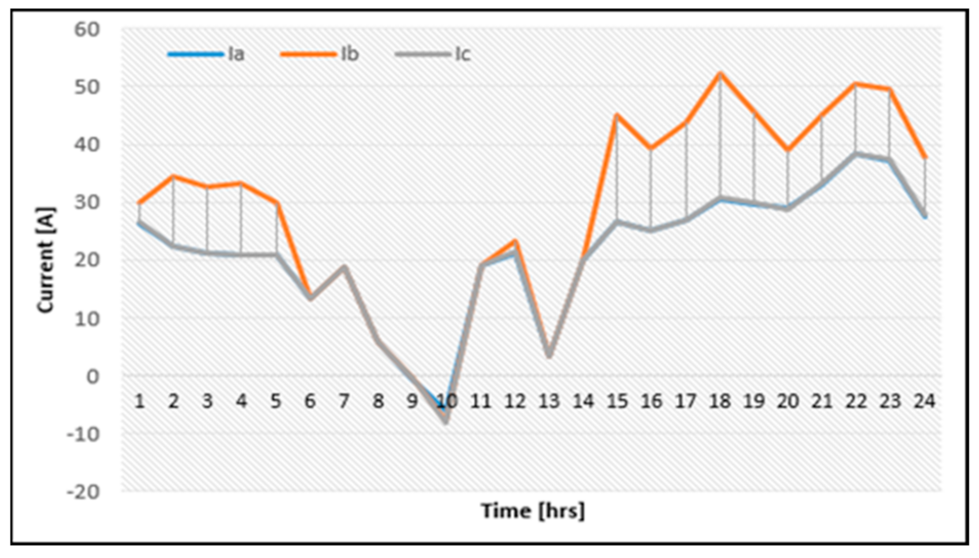
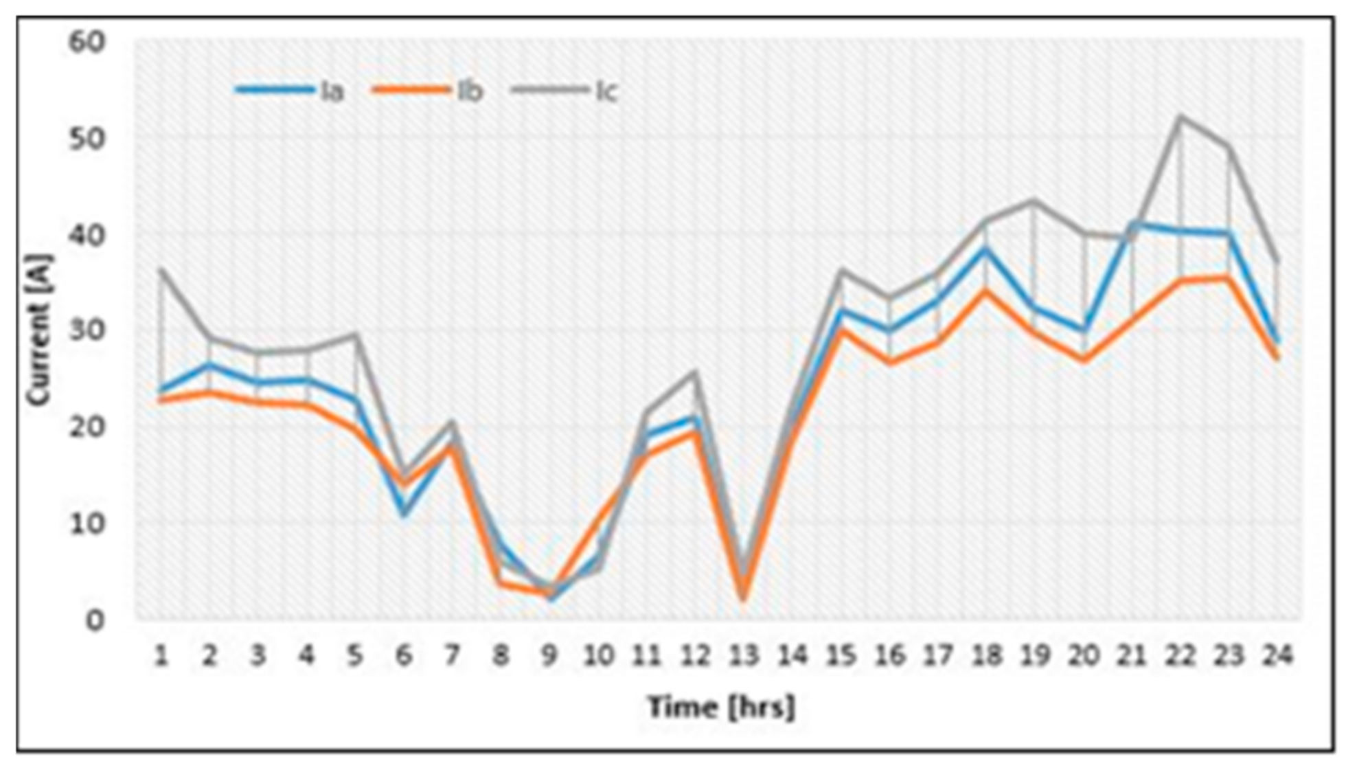
Hour	W-PLB				P-PLB				C-PLB				H-PLB
	Ia	Ib	Ic	UF	Ia	Ib	Ic	UF	Ia	Ib	Ic	UF	Ia	Ib	Ic	UF
H1	14.75	48.48	19.44	1.29	26.36	29.86	26.46	1.003	23.69	22.78	36.20	1.049	27.68	27.51	27.47	1.00001
H2	13.99	46.35	18.61	1.29	22.26	34.44	22.25	1.048	26.27	23.56	29.11	1.007	26.42	26.24	26.29	1.00001
H3	13.22	43.63	17.70	1.29	20.99	32.52	21.04	1.048	24.57	22.34	27.63	1.008	24.96	24.78	24.81	1.00001
H4	13.35	44.21	17.42	1.30	20.79	33.37	20.81	1.056	24.91	22.28	27.79	1.008	25.09	24.94	24.95	1.00001
H5	12.76	41.49	17.60	1.27	20.93	29.99	20.92	1.032	22.71	19.65	29.49	1.029	23.95	23.86	24.04	1.00001
H6	6.49	19.18	14.24	1.15	13.32	13.24	13.35	1.000	10.90	13.91	15.09	1.018	13.28	13.38	13.25	1.00002
H7	11.84	27.22	17.21	1.12	18.81	18.66	18.80	1.000	18.25	17.73	20.30	1.003	18.81	18.64	18.83	1.00002
H8	3.97	−0.38	13.73	1.87	5.81	5.87	5.64	1.000	7.80	3.63	5.88	1.087	5.64	5.81	5.87	1.00028
H9	−1.41	−11.89	12.12	1.35	−0.50	−0.28	−0.39	1.052	2.14	2.59	3.55	1.046	0.31	0.31	0.30	1.00026
H10	−8.24	−23.45	9.54	1.25	−6.06	−7.99	−8.10	1.016	6.51	10.43	5.21	1.090	7.36	7.37	7.41	1.00001
H11	8.65	30.45	18.25	1.22	19.16	19.08	19.12	1.000	19.00	17.04	21.32	1.008	19.15	19.06	19.15	1.00000
H12	10.59	37.93	17.34	1.28	21.16	23.35	21.36	1.002	20.85	19.48	25.54	1.014	21.90	22.03	21.94	1.00001
H13	−2.81	0.84	11.79	1.86	3.26	3.20	3.36	1.000	2.97	2.20	4.65	1.097	3.27	3.21	3.35	1.00030
H14	8.62	32.81	18.05	1.25	19.78	19.84	19.86	1.000	19.54	18.29	21.65	1.005	19.82	19.79	19.86	1.00000
H15	17.25	58.91	21.88	1.33	26.55	44.87	26.62	1.070	31.91	29.97	36.16	1.006	32.80	32.62	32.61	1.00001
H16	15.64	52.93	21.03	1.30	25.01	39.38	25.21	1.051	29.83	26.50	33.26	1.009	29.83	29.89	29.87	1.00000
H17	17.48	58.20	22.08	1.31	26.93	43.85	26.98	1.060	33.13	28.67	35.96	1.008	32.71	32.54	32.51	1.00001
H18	21.50	66.45	25.74	1.29	30.60	52.35	30.74	1.073	38.49	34.04	41.16	1.006	37.94	37.96	37.80	1.00000
H19	21.27	58.94	25.08	1.23	29.72	45.66	29.91	1.045	32.27	29.74	43.28	1.028	35.19	34.98	35.12	1.00001
H20	21.23	51.61	23.72	1.18	28.91	38.88	28.77	1.022	29.83	26.74	39.98	1.031	32.11	32.25	32.20	1.00000
H21	25.60	58.45	27.01	1.17	32.91	45.02	33.13	1.023	40.88	30.87	39.32	1.014	36.86	37.18	37.03	1.00001
H22	27.62	68.09	31.47	1.19	38.28	50.47	38.43	1.018	40.18	35.07	51.94	1.028	42.56	42.24	42.38	1.00001
H23	24.77	68.72	30.58	1.22	37.30	49.44	37.33	1.019	39.93	35.23	48.90	1.019	41.25	41.23	41.58	1.00002
H24	17.09	52.92	23.12	1.25	27.59	37.86	27.67	1.024	29.00	27.08	37.05	1.019	30.91	30.99	31.22	1.00002

* W-PLB: without PLB; P-PLB: prosumer-level PLB; C-PLB: consumer-level PLB; and H-PLB: hybrid-level PLB.

contains details regarding the hourly values of the phase currents and UF at the level of the CCP obtained in all analysed cases: without PLB (W-PLB), P-PLB, C-PLB, and H-PLB.

In the final stage, the quantification of the technical benefits obtained after applying the PLB algorithm has been achieved through energy savings and the phase voltage unbalance rate at the end poles (P88 and P39). The energy-saving has been calculated based on the following formula:

$$E{S}_{PLB}=\left|\frac{\Delta W_{W-PLB}-\Delta W_{PLB}}{\Delta W_{W-PLB}}\right|\cdot 100,[\%]$$

(9)

where ΔW_PLB represents the energy losses calculated after the application of the PLB algorithm for the cases P-PLB, C-PLB, and H-PLB, and ΔW_W-PLB relates to the energy losses calculated for the initial situation, without PLB (W-PLB).

The energy losses have been calculated with an efficient steady-state algorithm based on the forward/backward sweep procedure proposed in [37] for the balanced and unbalanced AEDNs with four wires.

Table 8. Comparison between the technical indicators of the AEDN in the analysed cases.

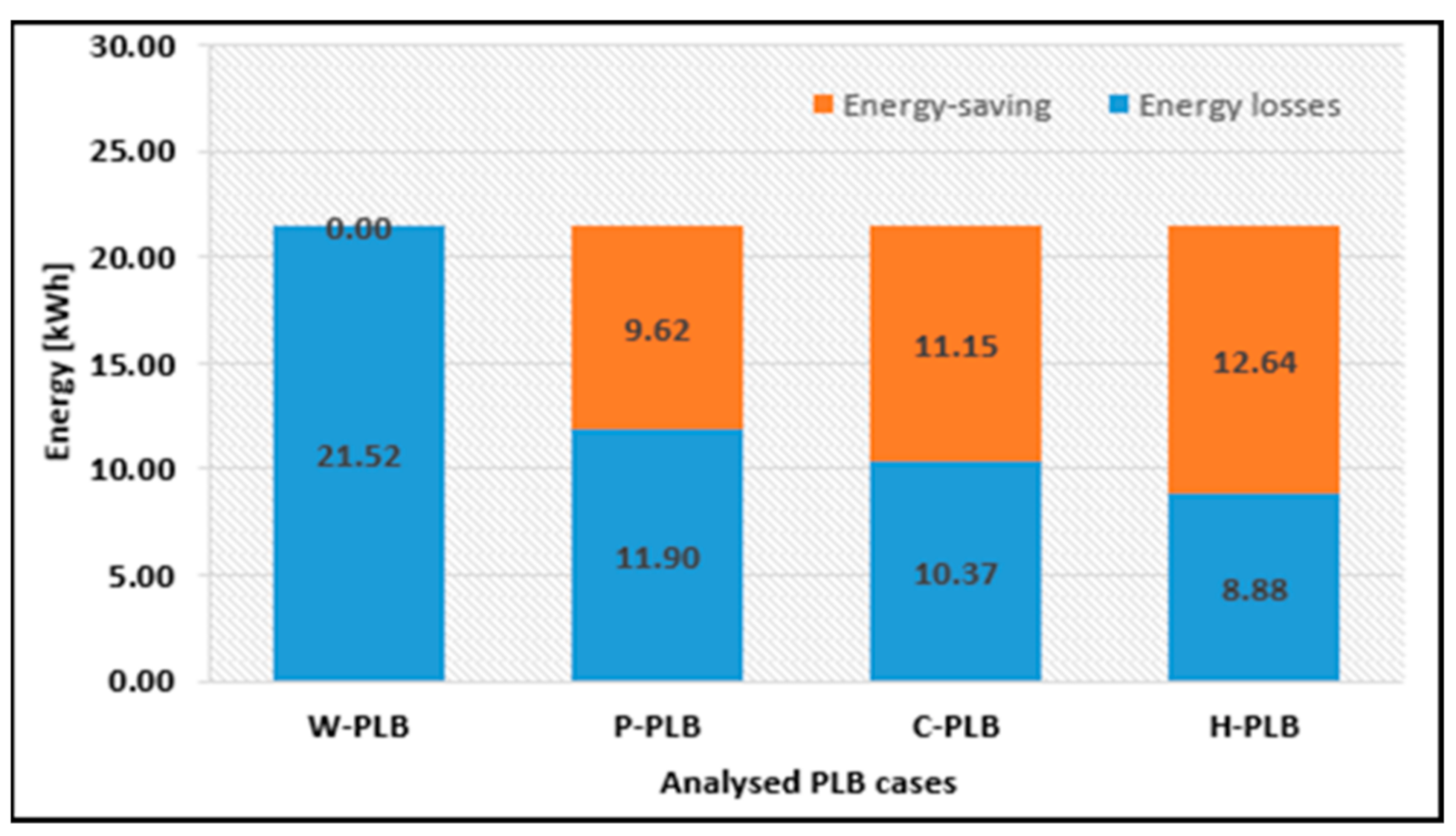
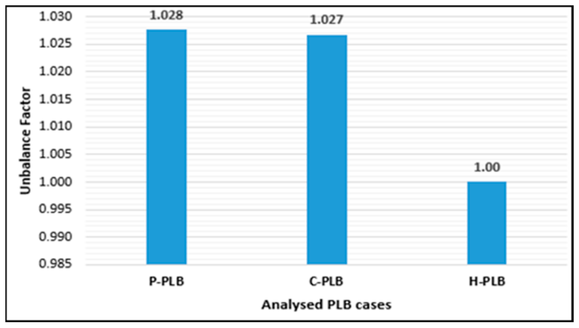
Case	UFav	ΔW (kWh)	ESPLB
			(kWh)	(%)
W-PLB	1.260	21.52	-	-
P-PLB	1.028	11.90	9.62	44.70
C-PLB	1.027	10.37	11.15	51.82
H–PLB	1.000	8.88	12.64	58.73

and Figure 21 present a comparison between the PLB algorithm considering the average value of the unbalance factor (UF_av), the energy losses (ΔW), and energy-saving (ES_PLB). The highest benefits have been recorded using the proposed H-PLB algorithm quantified through an energy-saving of 12.64 kWh in an analysed interval (24 h), representing 58.73% of the energy losses calculated in the initial situation (without PLB). The value is higher than the C-PLB algorithm by 6.91%, and by 14.03% compared with the P-PLB algorithm.

Table 9. The hourly total power losses calculated for all analysed cases, in (kW).

Hour	PLB Cases				Hour	PLB Cases
	W-PLB	P-PLB	C-PLB	H-PLB		W-PLB	P-PLB	C-PLB	H-PLB
H1	0.89	0.46	0.44	0.37	H13	0.19	0.18	0.15	0.10
H2	0.81	0.43	0.37	0.32	H14	0.50	0.27	0.29	0.22
H3	0.72	0.37	0.33	0.29	H15	1.28	0.67	0.56	0.49
H4	0.73	0.38	0.33	0.29	H16	1.05	0.55	0.48	0.42
H5	0.66	0.34	0.31	0.27	H17	1.26	0.67	0.56	0.50
H6	0.23	0.11	0.16	0.10	H18	1.69	0.91	0.75	0.67
H7	0.40	0.19	0.24	0.18	H19	1.40	0.75	0.64	0.57
H8	0.20	0.19	0.14	0.09	H20	1.14	0.59	0.55	0.49
H9	0.27	0.33	0.15	0.10	H21	1.50	0.79	0.72	0.65
H10	0.42	0.52	0.22	0.18	H22	2.03	1.04	0.98	0.87
H11	0.47	0.33	0.29	0.21	H23	1.99	0.99	0.91	0.83
H12	0.58	0.28	0.30	0.23	H24	1.12	0.56	0.51	0.45

contains details on the hourly total power losses calculated for all analysed cases.

The phase voltage unbalance rate (PVUR) has been evaluated according to the IEEE definition [44,45],

$$PVUR=\frac{\Delta V_{\max }}{V_{av}}\cdot 100,[\%]$$

(10)

where V_av is the average value of the phase voltage, and ΔV_max represents the maximum voltage deviation from the average value of the phase voltage.

Figure 22 and

Table 10. The average values of the PVUR calculated at the level of each pole from in the analysed cases, in (%).

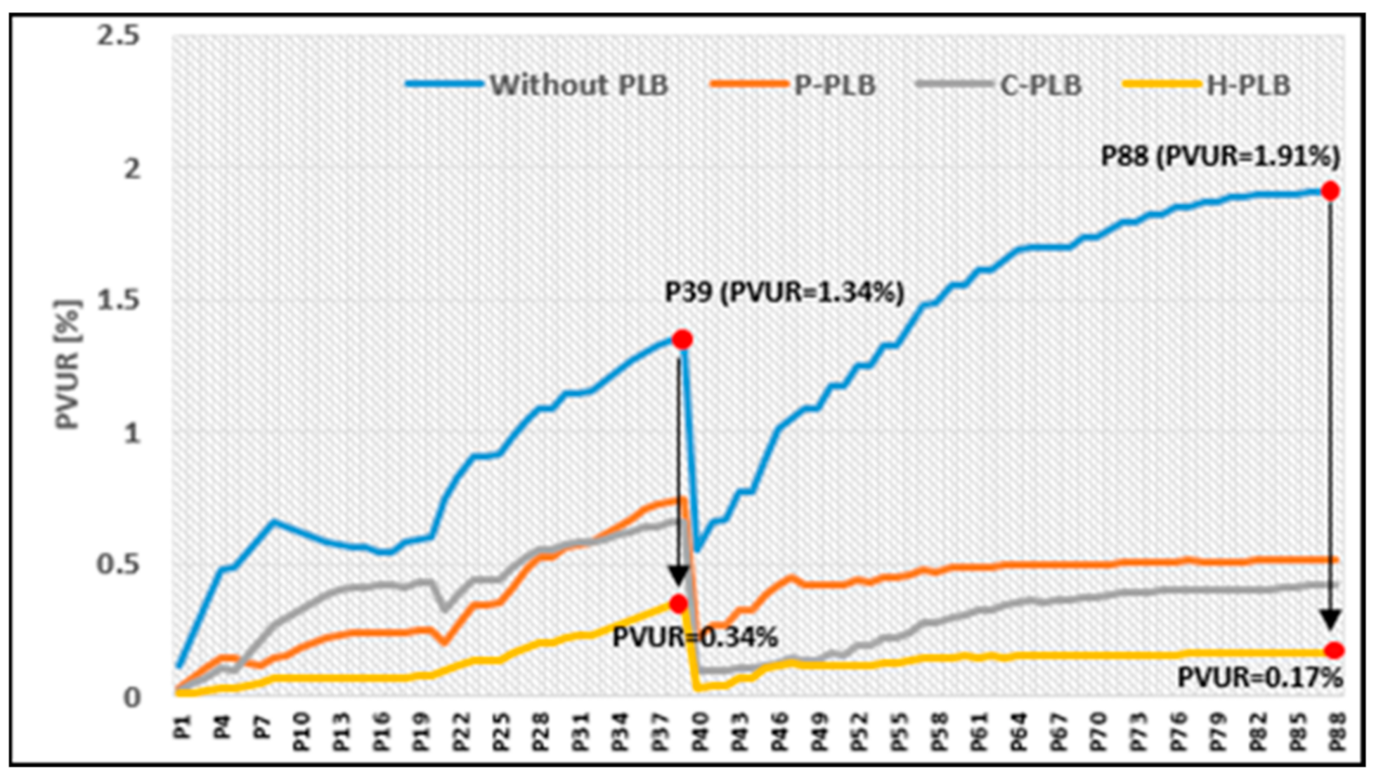
Pole	PLB Cases				Pole	PLB Cases
	W-PLB	P-PLB	C-PLB	H-PLB		W-PLB	P-PLB	C-PLB	H-PLB
P1	0.11	0.03	0.02	0.01	P45	0.90	0.38	0.12	0.10
P2	0.23	0.07	0.05	0.01	P46	1.01	0.42	0.13	0.11
P3	0.34	0.10	0.07	0.02	P47	1.05	0.45	0.14	0.12
P4	0.48	0.15	0.10	0.03	P48	1.09	0.42	0.14	0.11
P5	0.48	0.15	0.10	0.03	P49	1.09	0.42	0.14	0.11
P6	0.54	0.12	0.15	0.04	P50	1.17	0.42	0.16	0.11
P7	0.60	0.11	0.21	0.05	P51	1.17	0.42	0.16	0.11
P8	0.66	0.14	0.27	0.07	P52	1.25	0.44	0.19	0.12
P9	0.64	0.16	0.30	0.07	P53	1.25	0.43	0.19	0.12
P10	0.62	0.18	0.33	0.07	P54	1.32	0.45	0.22	0.12
P11	0.61	0.20	0.36	0.07	P55	1.32	0.45	0.22	0.12
P12	0.58	0.22	0.38	0.07	P56	1.40	0.46	0.24	0.13
P13	0.57	0.23	0.40	0.07	P57	1.48	0.47	0.27	0.14
P14	0.56	0.24	0.41	0.07	P58	1.49	0.47	0.28	0.14
P15	0.56	0.24	0.41	0.07	P59	1.55	0.49	0.30	0.15
P16	0.55	0.24	0.42	0.07	P60	1.56	0.49	0.30	0.15
P17	0.55	0.24	0.42	0.07	P61	1.61	0.49	0.32	0.15
P18	0.58	0.24	0.42	0.07	P62	1.61	0.49	0.32	0.15
P19	0.60	0.25	0.43	0.08	P63	1.65	0.49	0.34	0.15
P20	0.60	0.25	0.43	0.08	P64	1.69	0.50	0.36	0.15
P21	0.74	0.20	0.33	0.09	P65	1.69	0.50	0.36	0.15
P22	0.83	0.27	0.38	0.11	P66	1.69	0.50	0.36	0.15
P23	0.91	0.35	0.44	0.14	P67	1.70	0.50	0.36	0.15
P24	0.91	0.35	0.44	0.14	P68	1.70	0.50	0.36	0.15
P25	0.91	0.35	0.44	0.14	P69	1.73	0.50	0.37	0.15
P26	0.98	0.41	0.49	0.16	P70	1.73	0.50	0.37	0.15
P27	1.04	0.47	0.52	0.18	P71	1.77	0.50	0.38	0.15
P28	1.09	0.52	0.55	0.20	P72	1.79	0.50	0.39	0.15
P29	1.09	0.52	0.55	0.20	P73	1.79	0.50	0.39	0.15
P30	1.14	0.57	0.57	0.22	P74	1.82	0.51	0.39	0.16
P31	1.15	0.57	0.58	0.23	P75	1.82	0.51	0.40	0.16
P32	1.15	0.58	0.58	0.23	P76	1.84	0.51	0.40	0.16
P33	1.19	0.61	0.60	0.25	P77	1.85	0.51	0.40	0.16
P34	1.23	0.64	0.61	0.27	P78	1.86	0.51	0.40	0.16
P35	1.26	0.67	0.62	0.29	P79	1.86	0.51	0.40	0.16
P36	1.30	0.70	0.64	0.31	P80	1.88	0.51	0.40	0.16
P37	1.33	0.73	0.64	0.33	P81	1.89	0.51	0.40	0.16
P38	1.34	0.74	0.66	0.34	P82	1.89	0.51	0.41	0.17
P39	1.34	0.74	0.66	0.34	P83	1.89	0.51	0.41	0.17
P40	0.55	0.22	0.10	0.03	P84	1.90	0.51	0.41	0.17
P41	0.66	0.27	0.10	0.04	P85	1.90	0.51	0.41	0.17
P42	0.67	0.27	0.10	0.04	P86	1.90	0.51	0.42	0.17
P43	0.78	0.33	0.11	0.07	P87	1.90	0.51	0.42	0.17
P44	0.78	0.33	0.11	0.07	P88	1.91	0.51	0.42	0.17

present the average value of the PVUR in the analysed interval (24 h) at the level of each pole.

The highest decrease in the PVUR has been obtained in the case of the H-PLB algorithm. The PUVR has been improved from 1.34% to 0.34%, and from 1.91% to 0.17%, respectively, at the level of the end poles, P39 and P88.

4. Conclusions

The AEDNs integrate a high number of 1-P consumers, with a dynamic variation of the demand, and 1-P prosumers with different generation technologies, connected to the three phases, so that the phase currents are no longer equal, leading to current unbalance. Their effects can conduct to the inefficient network utilization, higher losses, higher neutral current, exceeding the allowable limits of the phase-neutral and phase-phase voltages, or difficulties in the voltage control.

The paper concentrated on the phase swapping measure, proposing an original centralized control methodology of the SSDs installed to all 1-P end-users to provide a fast PLB process in the AEDNs. The control of SSDs is achieved through a communication interface between the end-user and the network. The methodology allows the real-time query simultaneous of three different databases (Topology Database, SMS Database, and End-Users Database) of the DNO uploading the input data for a fast algorithm applied for all cases encountered in the PLB process (consumer-level, prosumer-level, or hybrid-level for all end-users) and the participation degree (depending on the absorbed/injected current, equal or different to 0, the 1-P end-user is or not considered in the PLB process). The 3-P prosumers and consumers were treated as the non-switchable end-users.

The methodology has been tested using an LV AEDN belonging to a Romanian DNO with 114 end-users integrated into the Smart Metering System during the day when the peak load has been recorded. The topology data (total length, number of the poles, and end-users) far exceed the average values associated with the AEDNs.

The performance associated with the time computing in the case of a full participation degree from the end-users (hybrid-level PLB) was better than that obtained in reference [15] (1.13 versus 1.26 s), where a similar heuristic PLB algorithm has been used and ran on an EDN having a similar topology. The UF at the level of the CCP has been improved, from 1.30 (unbalanced case, without PLB) to 1.00004. Additionally, the results have been compared with other possible PLB cases (the consumer-level PLB and prosumer-level PLB), obtaining similar values of the UF (1.028 vs. 1.027), slightly higher than in the hybrid-level PLB. However, all PLB cases lead to an unbalance degree below 1.1 (the target imposed by the DNO). Evaluation of the technical benefits highlighted the significant energy savings between 44.7% (the case of the prosumer-level PLB) and 58.73% (the case of the hybrid-level PLB). Additionally, the phase voltage unbalance rate decreased significantly, from the maximum value of 1.91% to 0.17% (the case of the hybrid-level PLB), 0.42% (the case of the consumer-level PLB), and 0.51% (the case of the prosumer-level PLB), at the level of the final pole. All results emphasized the effectiveness of the proposed control methodology.

However, their implementation in the AEDNs could be limited by the data communication infrastructure (it must have a high-speed), the master controller from the CCP (having the functions associated with high data acquisition and processing speed), and the 3-P branching for each 1-P end-user.

The authors’ future work will focus on the extension of the methodology, which considers the storage (or load flexibility) in the PLB process depending on various control configurations. The main objective is to include as many advanced technologies as possible to participate in the PLB process.

References

- Baker, P. Challenges Facing Distribution System Operators in a Decarbonised Power System. Regulatory Assistance Project. 2020. Available online: https://www.raponline.org/wp-content/uploads/2020/05/rap-baker-dso-challenges-june-2020-final.pdf (accessed on 7 September 2021).
- Liu, J.; Gao, H.; Ma, Z.; Li, Y. Review and prospect of active distribution system planning. J. Mod. Power Syst. Clean Energy 2015, 3, 457–467. [Google Scholar] [CrossRef] [Green Version]
- European Commission. Clean Energy for All Europeans Package. Available online: https://ec.europa.eu/energy/topics/energy-strategy/clean-energy-all-europeans_en (accessed on 18 November 2020).
- Internal Energy Agency. Digitalization & Energy. October 2017. Available online: https://iea.blob.core.windows.net/assets/b1e6600c-4e40-4d9c-809d-1d1724c763d5/DigitalizationandEnergy3.pdf (accessed on 7 September 2021).
- Li, R.; Wang, W.; Chen, Z.; Jiang, J.; Zhang, W. A Review of Optimal Planning Active Distribution System: Models, Methods, and Future Researches. Energies 2017, 10, 1715. [Google Scholar] [CrossRef] [Green Version]
- Mishra, D.K.; Ghadi, M.J.; Azizivahed, A.; Li, L.; Zhang, J. A review on resilience studies in active distribution systems. Renew. Sustain. Energy Rev. 2021, 135, 110201. [Google Scholar] [CrossRef]
- Beharrysingh, S. Phase Unbalance on Low-Voltage Electricity Networks and Its Mitigation Using Static Balancers. Ph.D. Thesis, Loughborough University, Loughborough, UK, 2014. Available online: https://dspace.lboro.ac.uk/dspace-jspui/handle/2134/16252 (accessed on 7 September 2021).
- Toader, C.; Porumb, R.; Bulac, C.; Tristiu, I. A perspective on current unbalance in low voltage distribution networks. In Proceedings of the 2015 9th International Symposium on Advanced Topics in Electrical Engineering (ATEE), Bucharest, Romania, 7–9 May 2015; pp. 741–746. [Google Scholar]
- Ojo, A.; Awodele, K.; Sebitosi, A. Load Compensation in a Three-Phase Four Wire Distribution System Considering Unbalance, Neutral Current Elimination and Power Factor Improvement. In Proceedings of the 2019 Southern African Universities Power Engineering Conference/Robotics and Mechatronics/Pattern Recognition Association of South Africa (SAUPEC/RobMech/PRASA), Bloemfontein, South Africa, 28–30 January 2019; pp. 389–394. [Google Scholar]
- Qudah, M.; Abu Elhaija, W.; Widyan, M. Performance analysis of different series compensation schemes of SMIB power system incorporating PV generator. Int. Trans. Electr. Energy Syst. 2021, 31, e12699. [Google Scholar] [CrossRef]
- Gebru, Y.; Bitew, D.; Aberie, H.; Gizaw, K. Performance enhancement of radial distribution system using simultaneous network reconfiguration and switched capacitor bank placement. Cogent Eng. 2021, 8, 1897929. [Google Scholar] [CrossRef]
- Vai, V.; Suk, S.; Lorm, R.; Chhlonh, C.; Eng, S.; Bun, L. Optimal Reconfiguration in Distribution Systems with Distributed Generations Based on Modified Sequential Switch Opening and Exchange. Appl. Sci. 2021, 11, 2146. [Google Scholar] [CrossRef]
- Shahnia, F.; Wolfs, P.; Ghosh, A. Voltage Unbalance Reduction in Low Voltage Feeders by Dynamic Switching of Residential Customers Among Three Phases. IEEE Trans. Smart Grid 2014, 5, 1318–1327. [Google Scholar] [CrossRef] [Green Version]
- Bao, G.; Ke, S. Load Transfer Device for Solving a Three-Phase Unbalance Problem Under a Low-Voltage Distribution Network. Energies 2019, 12, 2842. [Google Scholar] [CrossRef] [Green Version]
- Grigoraș, G.; Neagu, B.-C.; Gavrilaș, M.; Triștiu, I.; Bulac, C. Optimal Phase Load Balancing in Low Voltage Distribution Networks Using a Smart Meter Data-Based Algorithm. Mathematics 2020, 8, 549. [Google Scholar] [CrossRef] [Green Version]
- Liu, B.; Meng, K.; Dong, Z.Y.; Wong, P.K.C.; Li, X. Load Balancing in Low-Voltage Distribution Network via Phase Reconfiguration: An Efficient Sensitivity-Based Approach. IEEE Trans. Power Deliv. 2021, 36, 2174–2185. [Google Scholar] [CrossRef]
- Haq, S.U.; Arif, B.; Khan, A.; Ahmed, J. Automatic three phase load balancing system by using fast switching relay in three phase distribution system. In Proceedings of the 2018 1st International Conference on Power, Energy and Smart Grid (ICPESG), Mirpur Azad Kashmir, Pakistan, 9–10 April 2018; pp. 1–6. [Google Scholar]
- Homaee, O.; Najafi, A.; Dehghanian, M.; Attar, M.; Falaghi, H. A practical approach for distribution network load balancing by optimal re-phasing of single phase customers using discrete genetic algorithm. Int. Trans. Electr. Energy Syst. 2019, 29, e2834. [Google Scholar] [CrossRef]
- Grigoraș, G.; Neagu, B.-C.; Scarlatache, F.; Noroc, L.; Chelaru, E. Bi-Level Phase Load Balancing Methodology with Clustering-Based Consumers’ Selection Criterion for Switching Device Placement in Low Voltage Distribution Networks. Mathematics 2021, 9, 542. [Google Scholar] [CrossRef]
- Sureshkumar, R.; Maithili, P. Three Phase Load Balancing And Energy Loss Reduction In Distribution Network Using Labiew. Int. J. Pure Appl. Math. 2017, 116, 181–189. [Google Scholar]
- Abril, I.P. Multi-objective optimization of the balancing of phases in primary distribution circuits. Int. J. Electr. Power Energy Syst. 2016, 82, 420–428. [Google Scholar] [CrossRef]
- Singh, D.; Misra, R.K.; Mishra, S. Distribution system feeder re-phasing considering voltage-dependency of loads. Int. J. Electr. Power Energy Syst. 2016, 76, 107–119. [Google Scholar] [CrossRef]
- Siti, W.M.; Jimoh, A.; Nicolae, D. Distribution network phase load balancing as a combinatorial optimization problem using fuzzy logic and Newton–Raphson. Electr. Power Syst. Res. 2011, 81, 1079–1087. [Google Scholar] [CrossRef]
- Pan, J.; Liu, J.; Chen, X.; Zhong, K. Three-phase unbalanced load control based on load–electricity transfer index. Energy Rep. 2021, 7, 312–318. [Google Scholar] [CrossRef]
- Caldognetto, T.; Tenti, P.; Mattavelli, P.; Buso, S.; Brandao, D. Cooperative compensation of unwanted current terms in low-voltage microgrids by distributed power-based control. In Proceedings of the 2015 IEEE 13th Brazilian Power Electronics Conference and 1st Southern Power Electronics Conference (COBEP/SPEC), Fortaleza, Brazil, 29 November–2 December 2015; pp. 1–7. [Google Scholar]
- Brandao, D.I.; Caldognetto, T.; Marafão, F.; Simoes, M.G.; Pomilio, J.A.; Tenti, P. Centralized Control of Distributed Single-Phase Inverters Arbitrarily Connected to Three-Phase Four-Wire Microgrids. IEEE Trans. Smart Grid 2017, 8, 437–446. [Google Scholar] [CrossRef] [Green Version]
- Blaud, P.C.; Haurant, P.; Claveau, F.; Lacarrière, B.; Chevrel, P.; Mouraud, A. Modelling and control of multi-energy systems through Multi-Prosumer Node and Economic Model Predictive Control. Int. J. Electr. Power Energy Syst. 2020, 118, 105778. [Google Scholar] [CrossRef]
- Mieński, R.; Urbanek, P.; Wasiak, I. Using Energy Storage Inverters of Prosumer Installations for Voltage Control in Low-Voltage Distribution Networks. Energies 2021, 14, 1121. [Google Scholar] [CrossRef]
- Soltani, S.; Rashidinejad, M.; Abdollahi, A. Dynamic phase balancing in the smart distribution networks. Int. J. Electr. Power Energy Syst. 2017, 93, 374–383. [Google Scholar] [CrossRef]
- Wang, W.; Yu, N. Phase Balancing in Power Distribution Network with Data Center. ACM Sigmetrics Perform. Eval. Rev. 2017, 45, 64–69. [Google Scholar] [CrossRef]
- Chen, C.-S.; Tsai, C.-T.; Lin, C.-H.; Hsieh, W.-L.; Ku, T.-T. Loading Balance of Distribution Feeders With Loop Power Controllers Considering Photovoltaic Generation. IEEE Trans. Power Syst. 2011, 26, 1762–1768. [Google Scholar] [CrossRef]
- Charalambous, A.; Hadjidemetriou, L.; Zacharia, L.; Bintoudi, A.D.; Tsolakis, A.C.; Tzovaras, D.; Kyriakides, E. Phase Balancing and Reactive Power Support Services for Microgrids. Appl. Sci. 2019, 9, 5067. [Google Scholar] [CrossRef] [Green Version]
- Ciontea, C.; Iov, F. A Study of Load Imbalance Influence on Power Quality Assessment for Distribution Networks. Electricity 2021, 2, 77–90. [Google Scholar] [CrossRef]
- Kwaśny, L.; Zieliński, D. Control of a Four-wire Hybrid Prosumer Converter for Balancing Utility Grids. Power Electron. Drives 2021, 6, 1–11. [Google Scholar]
- Drabek, T.; Dybowski, P. Control of prosumer voltage sources in distribution grids. In Proceedings of the 2020 12th International Conference and Exhibition on Electrical Power Quality and Utilisation (EPQU), Cracow, Poland, 14–15 September 2020; pp. 1–6. [Google Scholar]
- Volosciuc, S.D.; Dragosin, M.E. Prosumer’s impact on low voltage distribution networks. Proc. MATEC Web Conf. EDP Sci. 2019, 290, 01021. [Google Scholar] [CrossRef] [Green Version]
- Grigoras, G.; Neagu, B.-C. Smart Meter Data-Based Three-Stage Algorithm to Calculate Power and Energy Losses in Low Voltage Distribution Networks. Energies 2019, 12, 3008. [Google Scholar] [CrossRef] [Green Version]
- Munakata, T.; Barták, R. Logic programming for combinatorial problems. Artif. Intell. Rev. 2010, 33, 135–150. [Google Scholar] [CrossRef] [Green Version]
- Shan, X. (Gene); Felder, F.A.; Coit, D.W. Game-theoretic models for electric distribution resiliency/reliability from a multiple stakeholder perspective. IISE Trans. 2017, 49, 159–177. [Google Scholar] [CrossRef]
- Romanian Energy Regulatory Authority, Report on the Performance Indicators for Electric Transmission, System and Distribution Services and the Technical State of Electric Transmission and Distribution Networks in 2018, Romania. 2019. Available online: https://www.anre.ro/ro/energie-electrica/rapoarte/rapoarte-indicatori-performanta (accessed on 15 September 2021). (In Romanian).
- Baričević, T.; Skok, M.; Majstrović, G.; Perić, K.; Brajković, J. South East European Distribution System Operators Benchmarking Study. Available online: https://www.usea.org/sites/default/files/SEE%20DSO%20Benchmarking%20Study%202008%20-%202015%20-%20final.pdf (accessed on 15 September 2021).
- Ivanov, O.; Grigoras, G.; Neagu, B.C. Smart Metering based Approaches to Solve the Load Phase Balancing Problem in Low Voltage Distribution Networks. In Proceedings of the 2018 International Symposium on Fundamentals of Electrical Engineering (ISFEE), Bucharest, Romania, 1–3 November 2018; pp. 1–6. [Google Scholar] [CrossRef]
- Ivanov, O.; Neagu, B.-C.; Gavrilas, M.; Grigoras, G.; Sfintes, C.-V. Phase Load Balancing in Low Voltage Distribution Networks Using Metaheuristic Algorithms. In Proceedings of the 2019 International Conference on Electromechanical and Energy Systems (SIELMEN), Craiova, Romania, 9–11 October 2019; pp. 1–6. [Google Scholar]
- Pillay, P.; Manyage, M. Definitions of voltage unbalance. IEEE Power Eng. Rev. 2001, 21, 50–51. [Google Scholar] [CrossRef]
- Bollen, M. Definitions of voltage unbalance. IEEE Power Eng. Rev. 2002, 22, 49–50. [Google Scholar] [CrossRef]