
The Log Exponential-Power Distribution: Properties, Estimations and Quantile Regression Model


Abstract
:1. Introduction
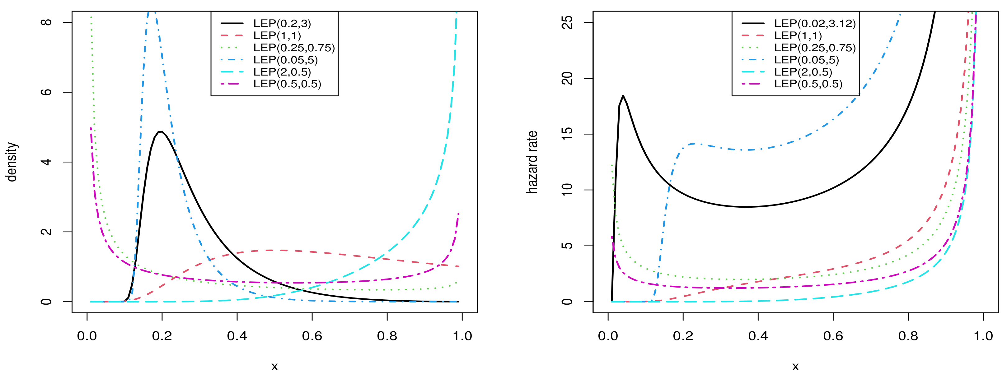
2. Some Distributional Properties of the LEP Distribution
2.1. Moments
2.2. Order Statistics
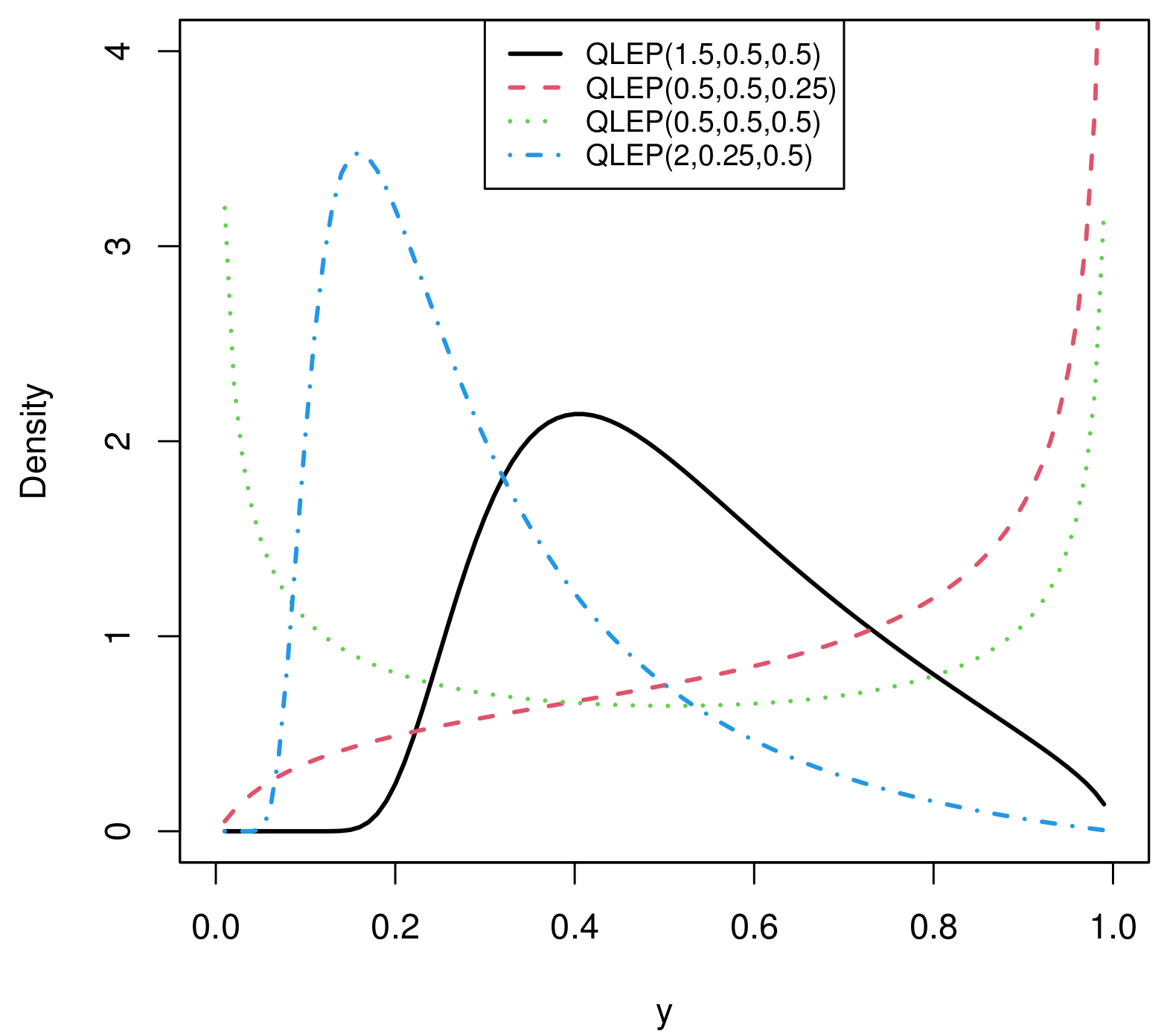
2.3. Quantile Function and Quantile LEP Distribution
2.4. Residual Entropy and Cumulative Residual Entropy
3. Procedure of the Maximum Likelihood for the Parameter Estimation
4. The New Quantile Regression Model Based on the QLEP Distribution for the Unit Response
4.1. The MLEs of the Model Parameters
4.2. Model Validity for the Fitting
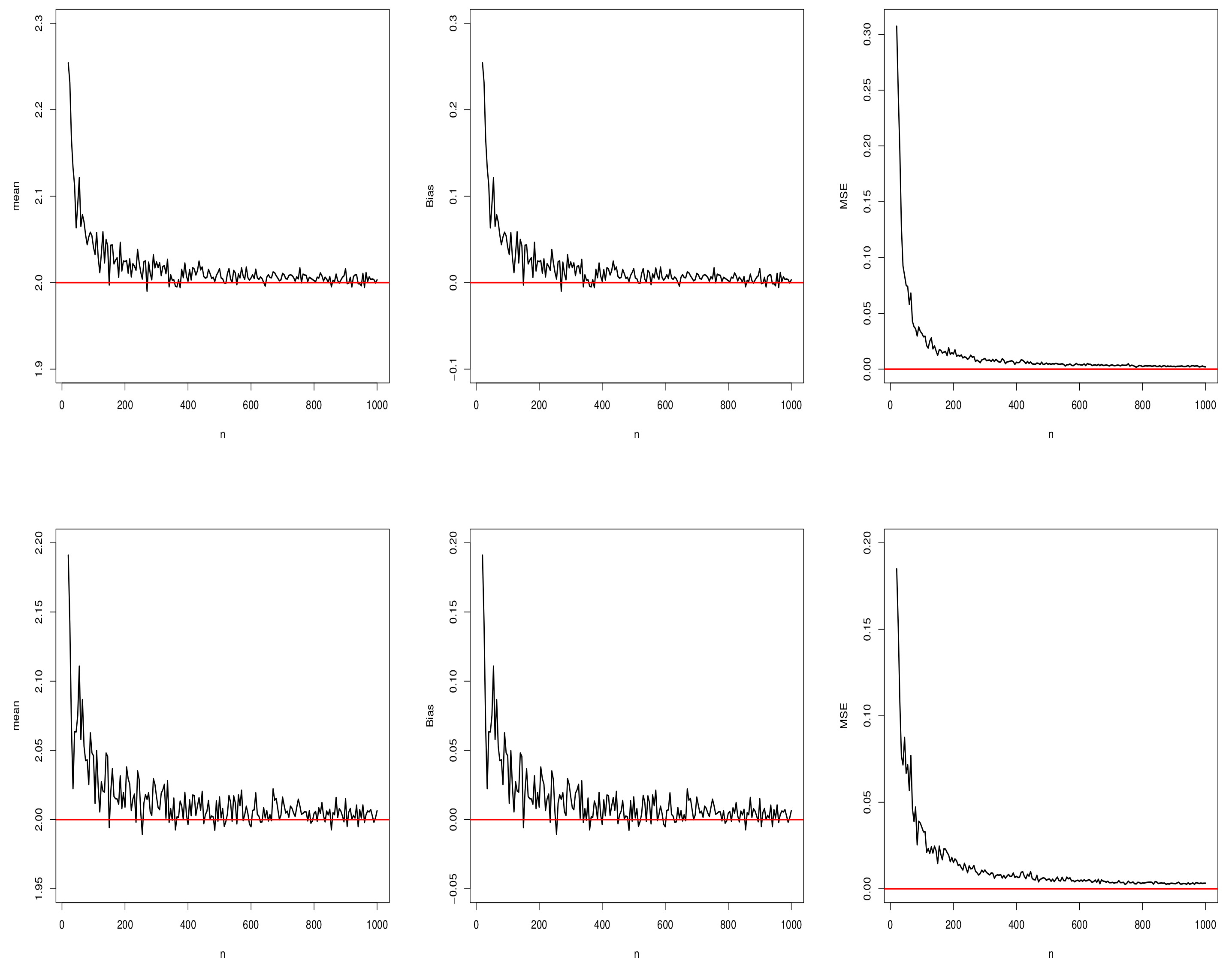
5. Simulation Studies
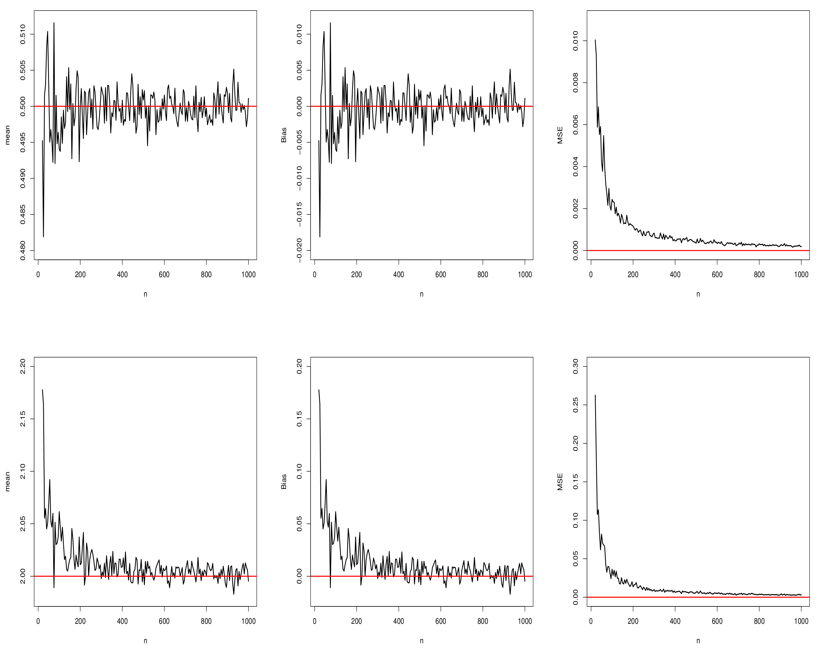
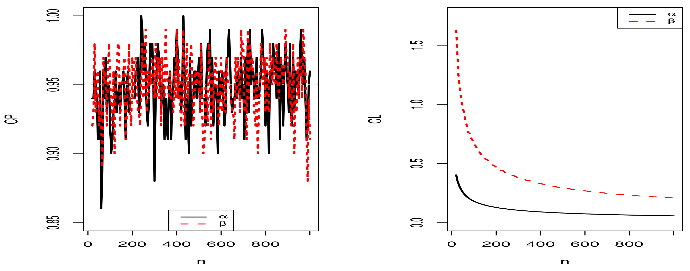
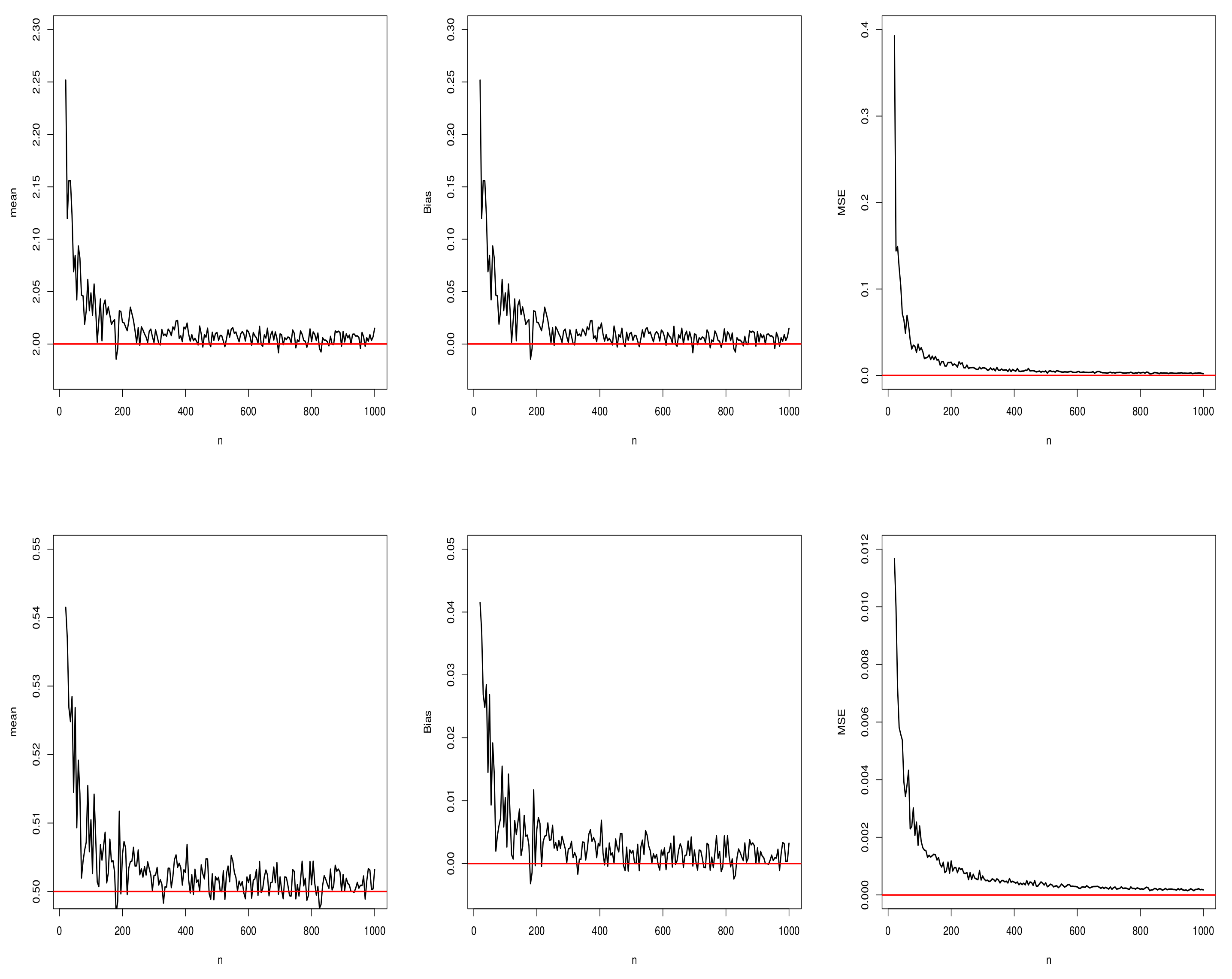
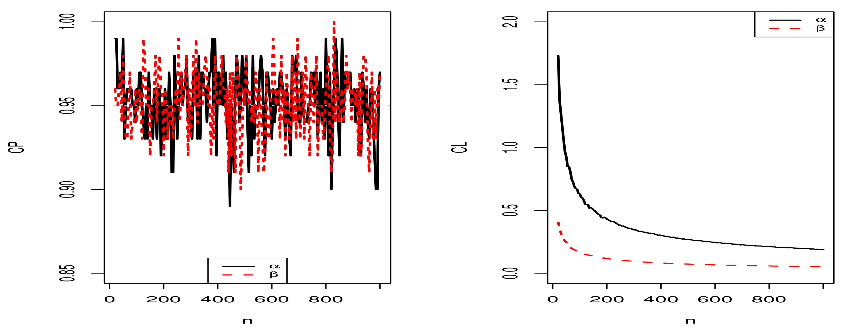
5.1. Simulation Results for the MLEs of the Proposed Distribution
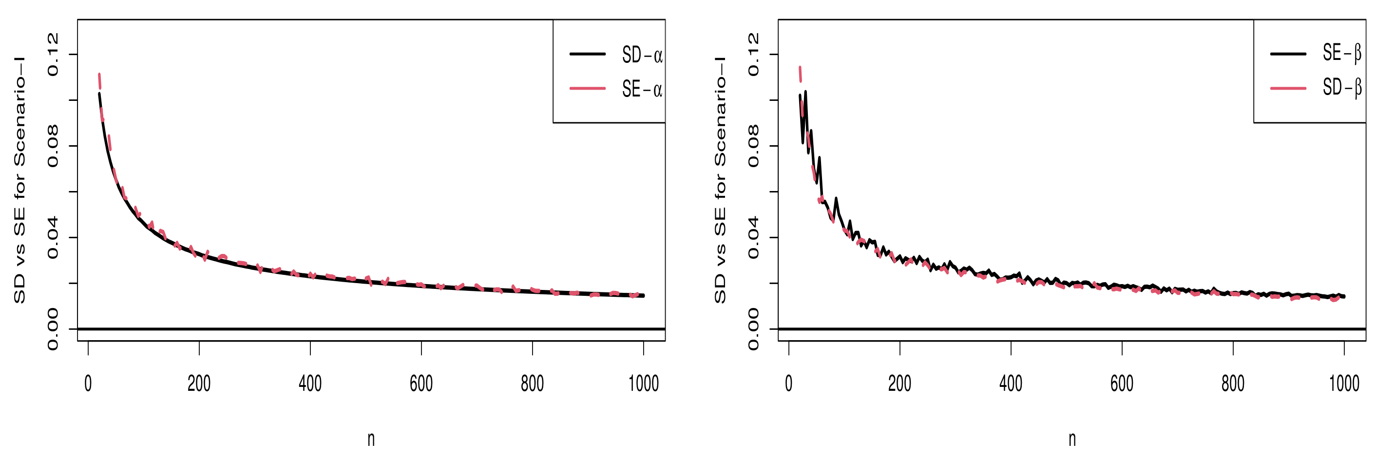
5.1.1. Scenario I
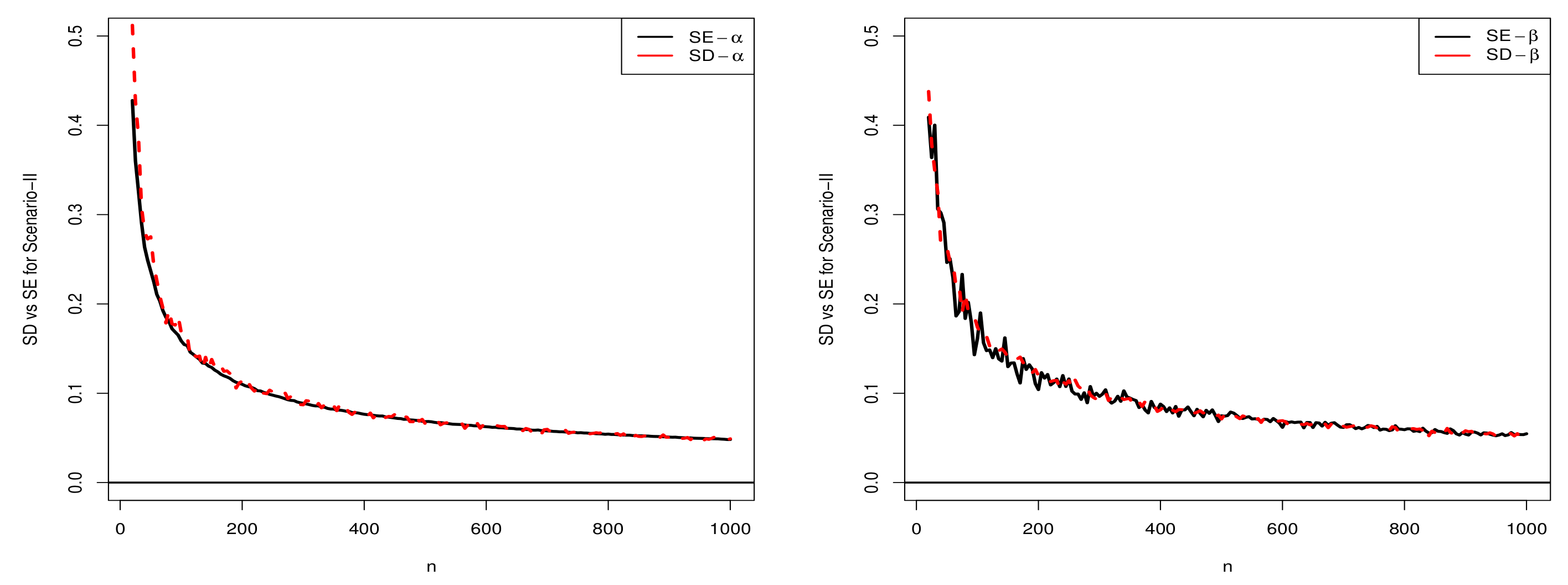
5.1.2. Scenario II
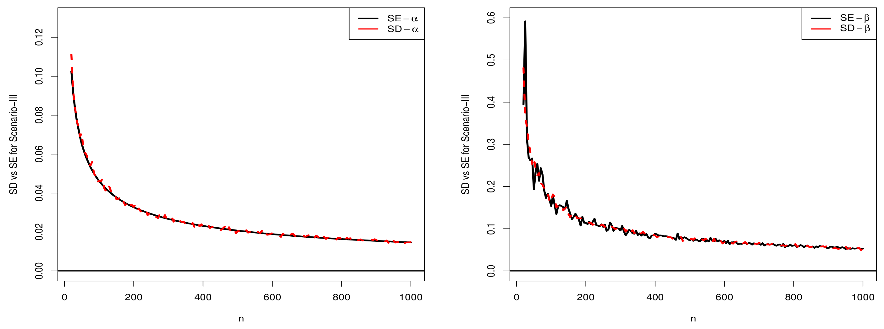
5.1.3. Scenario III
5.1.4. Scenario IV
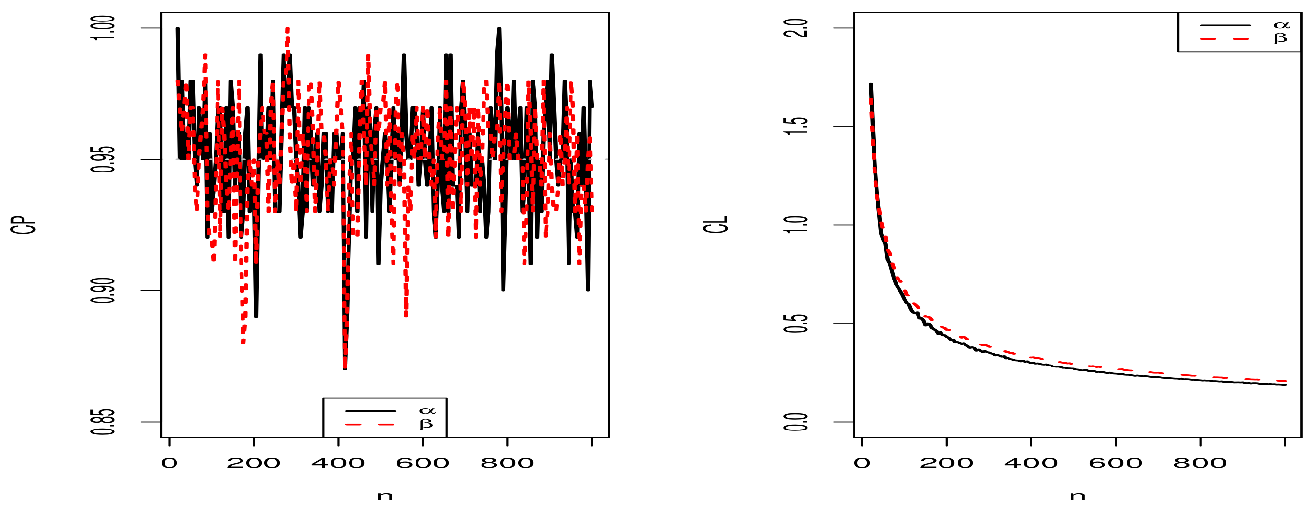
5.2. Comparison of SD and SE
5.3. Simulation Studies for the Proposed Regression Model
6. Applications
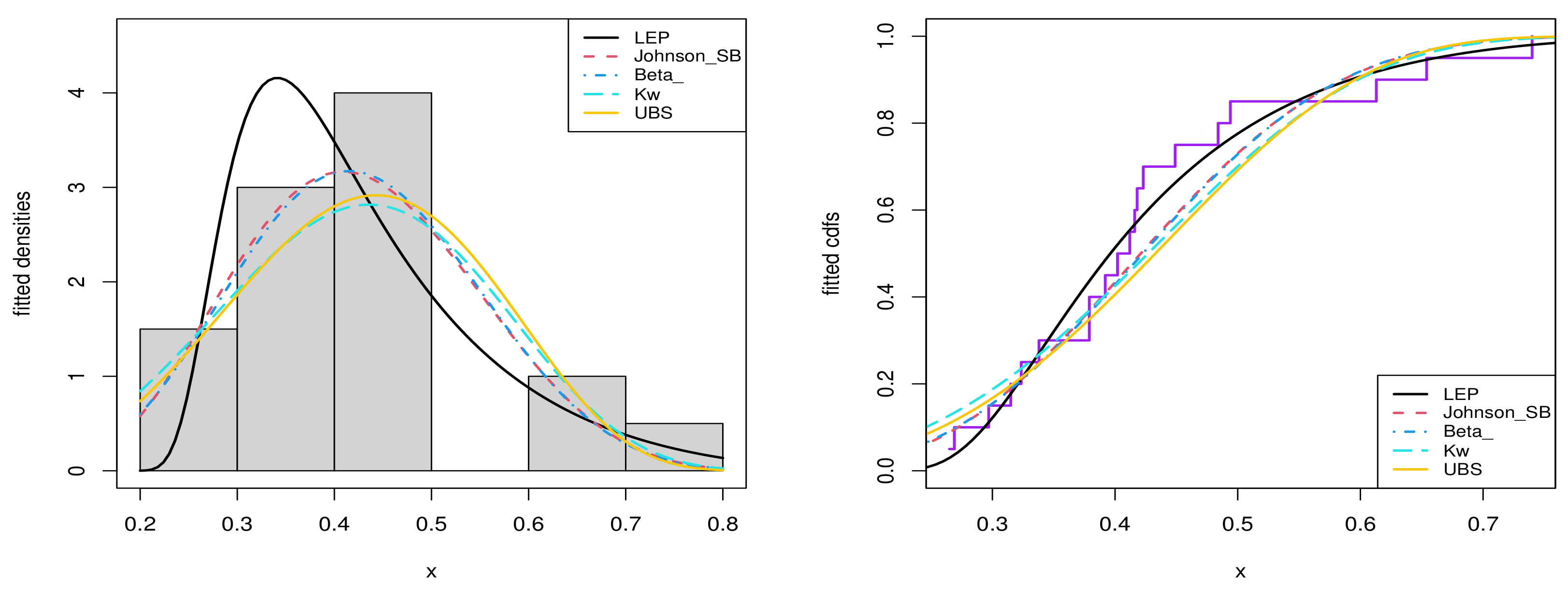
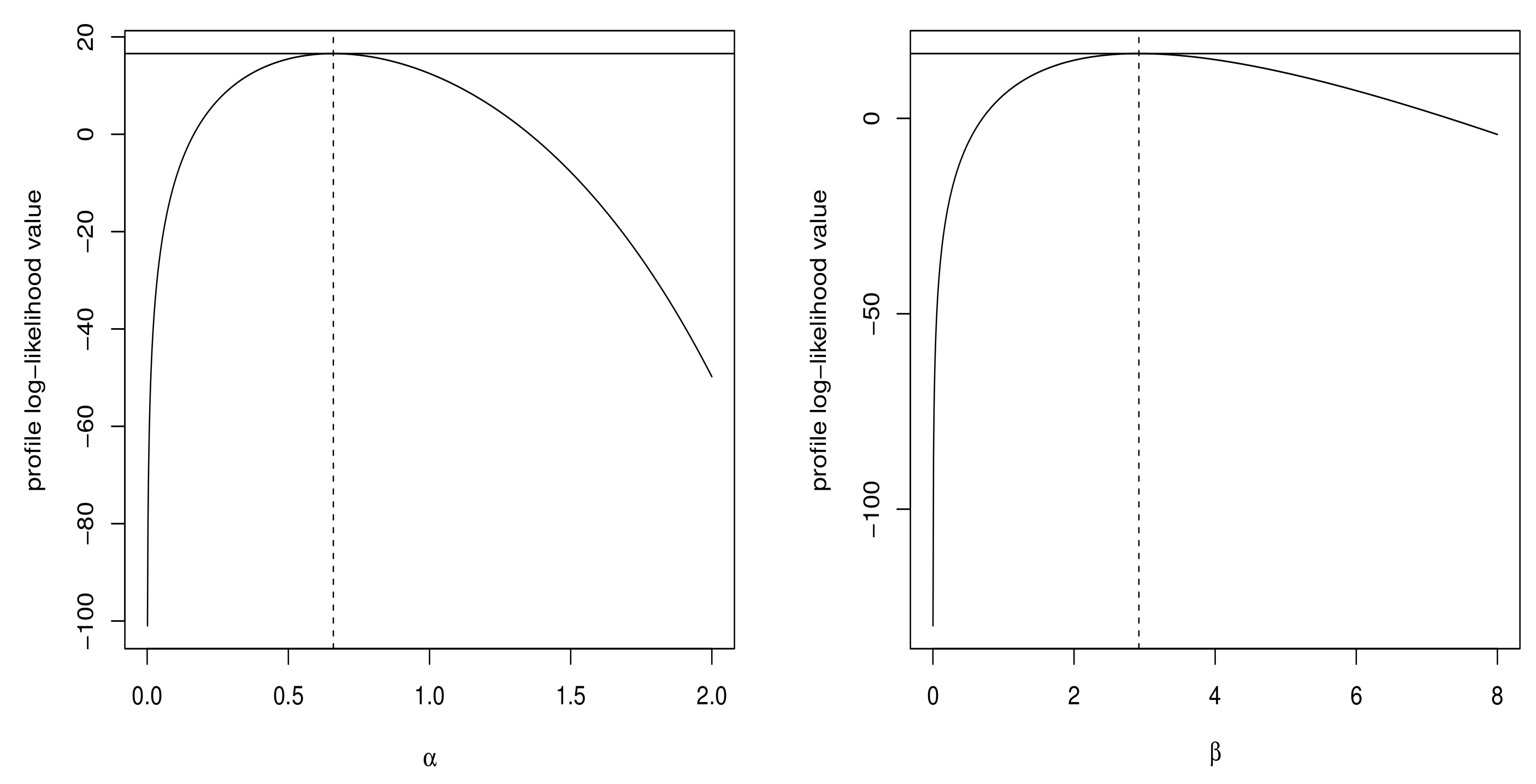
6.1. Real Data Application for the Univariate Data Modeling
- Beta distribution:and for , where , , and is the standard beta function.
- Kumaraswamy (Kw) distribution [34]:and for , where and .
- Johnson distribution [35]:and for , where , , and the is the pdf of the standard normal distribution.
- Unit Birnbaum Saunders () distribution [36]:and for , where and .
6.2. Quantile Regression Application
7. Conclusions
Author Contributions
Funding
Institutional Review Board Statement
Informed Consent Statement
Data Availability Statement
Conflicts of Interest
References
- Smith, R.M.; Bain, L.J. An exponential power life-testing distribution. Commun. Stat. Theory Methods 1975, 4, 469–481. [Google Scholar]
- Shakil, M.; Ahsanullah, M.; Kibria, B.G. On the Characterizations of Chen’s Two-Parameter Exponential Power Life-Testing Distribution. J. Stat. Theory Appl. 2018, 17, 393–407. [Google Scholar]
- Saraçoğlu, B.; Taniş, C. A new lifetime distribution: Transmuted exponential power distribution. Commun. Fac. Sci. Univ. Ank. Ser. Math. Stat. 2021, 70, 1–14. [Google Scholar]
- Taniş, C.; Saraçoğlu, B.; Coşkun, K.; Pekgör, A. Transmuted complementary exponential power distribution: Properties and applications. Cumhur. Sci. J. 2020, 41, 419–432. [Google Scholar] [CrossRef]
- Abd El-Monsef, M.; El-Awady, M. Generalized Exponential Power Distribution with Application to Complete and Censored Data. Asian J. Probab. Stat. 2021, 34–55. [Google Scholar] [CrossRef]
- Altun, E. The log-weighted exponential regression model: Alternative to the beta regression model. Commun. Stat. Theory Methods 2021, 50, 2306–2321. [Google Scholar] [CrossRef]
- Altun, E.; El-Morshedy, M.; Eliwa, M.S. A new regression model for bounded response variable: An alternative to the beta and unit-Lindley regression models. PLoS ONE 2021, 16, e0245627. [Google Scholar] [CrossRef]
- Altun, E.; Cordeiro, G.M. The unit-improved second-degree Lindley distribution: Inference and regression modeling. Comput. Stat. 2020, 35, 259–279. [Google Scholar] [CrossRef]
- Korkmaz, M.Ç.; Emrah, A.; Chesneau, C.; Yousof, H.M. On the unit-Chen distribution with associated quantile regression and applications. Math. Solovaca 2021. accepted paper. [Google Scholar]
- Altun, E.; Hamedani, G. The log-xgamma distribution with inference and application. J. Soc. Française Stat. 2018, 159, 40–55. [Google Scholar]
- Mazucheli, J.; Leiva, V.; Alves, B.; Menezes, A.F.B. A new quantile regression for modeling bounded data under a unit Birnbaum–Saunders distribution with applications in medicine and politics. Symmetry 2021, 13, 682. [Google Scholar] [CrossRef]
- Korkmaz, M.Ç.; Chesneau, C.; Korkmaz, Z.S. On the Arcsecant Hyperbolic Normal Distribution. Properties, Quantile Regression Modeling and Applications. Symmetry 2021, 13, 117. [Google Scholar] [CrossRef]
- Bakouch, H.S.; Nik, A.S.; Asgharzadeh, A.; Salinas, H.S. A flexible probability model for proportion data: Unit-Half-Normal distribution. Commun. Stat. Case Stud. Data Anal. Appl. 2021, 7, 271–288. [Google Scholar]
- Korkmaz, M.Ç.; Chesneau, C. On the unit Burr-XII distribution with the quantile regression modeling and applications. Comput. Appl. Math. 2021, 40, 29. [Google Scholar] [CrossRef]
- Korkmaz, M.Ç. The unit generalized half normal distribution: A new bounded distribution with inference and application. Appl. Math. Phys. 2020, 2, 133–140. [Google Scholar]
- Mazucheli, J.; Bapat, S.R.; Menezes, A.F.B. A new one-parameter unit-Lindley distribution. Chil. J. Stat. 2019, 11, 53–67. [Google Scholar]
- Gómez-Déniz, E.; Sordo, M.A.; Calderín-Ojeda, E. The Log-Lindley distribution as an alternative to the beta regression model with applications in insurance. Insur. Math. Econ. 2014, 54, 49–57. [Google Scholar] [CrossRef]
- Mazucheli, J.; Menezes, A.F.B.; Ghitany, M.E. The unit-Weibull Distribution and associated inference. J. Appl. Probab. Stat. 2018, 13, 1–22. [Google Scholar]
- Mazucheli, J.; Menezes, A.F.; Dey, S. Unit-Gompertz distribution with applications. Statistica 2019, 79, 25–43. [Google Scholar]
- MacDonald, I.L. Does Newton–Raphson really fail? Stat. Methods Med. Res. 2014, 23, 308–311. [Google Scholar] [CrossRef]
- Ferrari, S.; Cribari Neto, F. Beta regression for modelling rates and proportions. J. Appl. Stat. 2004, 31, 799–815. [Google Scholar] [CrossRef]
- Bayes, C.L.; Bazán, J.L.; García, C. A new robust regression model for proportions. Bayesian Anal. 2012, 7, 841–866. [Google Scholar] [CrossRef]
- Mazucheli, J.; Menezes, A.F.B.; Chakraborty, S. On the one parameter unit-Lindley distribution and its associated regression model for proportion data. J. Appl. Stat. 2019, 46, 700–714. [Google Scholar] [CrossRef] [Green Version]
- Koenker, R.; Bassett, G.J. Regression quantiles. Econ. J. Econ. Soc. 1978, 46, 33–50. [Google Scholar] [CrossRef]
- Mitnik, P.A.; Baek, S. The Kumaraswamy distribution: Median-dispersion re-parameterizations for regression modeling and simulation-based estimation. Stat. Pap. 2013, 54, 177–192. [Google Scholar] [CrossRef]
- Bayes, C.L.; Bazán, J.L.; Castro, M. A quantile parametric mixed regression model for bounded response variables. Stat. Its Interface 2017, 10, 483–493. [Google Scholar] [CrossRef]
- Mazucheli, J.; Menezes, A.F.B.; Fernandes, L.B.; de Oliveira, R.P.; Ghitany, M.E. The unit-Weibull distribution as an alternative to the Kumaraswamy distribution for the modeling of quantiles conditional on covariates. J. Appl. Stat. 2020, 47, 954–974. [Google Scholar] [CrossRef]
- Jodrá, P.; Jiménez-Gamero, M.D. A quantile regression model for bounded responses based on the Exponential-Geometric distribution. Revstat-Stat. J. 2020, 4, 415–436. [Google Scholar]
- Korkmaz, M.; Chesneau, C.; Korkmaz, Z. Transmuted unit Rayleigh quantile regression model: Alternative to beta and Kumaraswamy quantile regression models. Univ. Politeh. Buchar. Sci. Bull. Ser. Appl. Math. Phys. 2021, 83, 149–158. [Google Scholar]
- Dunn, P.K.; Smyth, G.K. Randomized quantile residuals. J. Comput. Graph. Stat. 1996, 5, 236–244. [Google Scholar]
- Cox, D.R.; Snell, E.J. A general definition of residuals. J. R. Stat. Soc. Ser. B (Methodol.) 1968, 30, 248–265. [Google Scholar] [CrossRef]
- Balakrishnan, N.; Cohen, A.C. Order Statistics & Inference: Estimation Methods; Elsevier: Amsterdam, The Netherlands, 2014. [Google Scholar]
- Alizadeh, M.; Altun, E.; Cordeiro, G.M.; Rasekhi, M. The odd power cauchy family of distributions: Properties, regression models and applications. J. Stat. Comput. Simul. 2018, 88, 785–807. [Google Scholar] [CrossRef]
- Kumaraswamy, P. A generalized probability density function for double-bounded random processes. J. Hydrol. 1980, 46, 79–88. [Google Scholar] [CrossRef]
- Johnson, N.L. Systems of frequency curves generated by methods of translation. Biometrika 1949, 36, 149–176. [Google Scholar] [CrossRef]
- Mazucheli, J.; Menezes, A.F.B.; Dey, S. The unit-Birnbaum-Saunders distribution with applications. Chil. J. Stat. 2018, 9, 47–57. [Google Scholar]
- Ouimet, M. A world of homicides: The effect of economic development, income inequality, and excess infant mortality on the homicide rate for 165 countries in 2010. Homicide Stud. 2012, 16, 238–258. [Google Scholar] [CrossRef]
- Mitra, D.; Kundu, D.; Balakrishnan, N. Likelihood analysis and stochastic EM algorithm for left truncated right censored data and associated model selection from the Lehmann family of life distributions. Jpn. J. Stat. Data Sci. 2021, 1–30. [Google Scholar]


| n | Bias- | Bias- | Bias- | MSE- | MSE- | MSE- | CL- | CL- | CL- | CP- | CP- | CP- |
| 25 | ||||||||||||
| 50 | ||||||||||||
| 100 | ||||||||||||
| 250 | ||||||||||||
| 500 | ||||||||||||
| n | Bias- | Bias- | Bias- | MSE- | MSE- | MSE- | CL- | CL- | CL- | CP- | CP- | CP- |
| 25 | ||||||||||||
| 50 | ||||||||||||
| 100 | - | |||||||||||
| 250 | - | |||||||||||
| 500 | ||||||||||||
| n | Bias- | Bias- | Bias- | MSE- | MSE- | MSE- | CL- | CL- | CL- | CP- | CP- | CP- |
| 25 | - | |||||||||||
| 50 | ||||||||||||
| 100 | − .0025 | |||||||||||
| 250 | − .0018 | |||||||||||
| 500 | ||||||||||||
| Model | ||||||||
|---|---|---|---|---|---|---|---|---|
| LEP | 0.6593 | 2.9194 | 16.5800 | −29.1593 | −28.4534 | 0.2923 | 0.0498 | 0.1366 |
| (0.1128) | (0.5537) | |||||||
| Johnson | 0.6143 | 1.9261 | 14.2629 | −24.5257 | −22.5342 | 0.6932 | 0.1154 | 0.1935 |
| (0.2438) | (0.3035) | |||||||
| Beta | 6.7568 | 9.1114 | 14.0622 | −24.1244 | −22.1330 | 0.7327 | 0.1236 | 0.1988 |
| (2.7299) | (3.4697) | |||||||
| 0.3783 | 0.8374 | 12.6784 | −21.3568 | −19.3653 | 1.0516 | 0.1898 | 0.2286 | |
| (0.0598) | 0.0696 | |||||||
| Kw | 3.3632 | 11.7892 | 12.8662 | −21.7324 | −19.7409 | 0.9322 | 0.1636 | 0.2109 |
| (0.6143) | (5.4906) |
| Parameters | QLEP | Kumaraswamy | Unit-Weibull | ||||||
|---|---|---|---|---|---|---|---|---|---|
| Estimates | SEs | p-Values | Estimates | SEs | p-Values | Estimates | SEs | p-Values | |
| −1.794 | 2.097 | 0.196 | 0.149 | 2.484 | 0.476 | -2.938 | 2.351 | 0.106 | |
| −0.025 | 0.031 | 0.208 | −0.034 | 0.035 | 0.167 | -0.004 | 0.034 | 0.456 | |
| −0.026 | 0.014 | 0.031 | −0.048 | 0.011 | <0.001 | -0.034 | 0.015 | 0.010 | |
| −0.004 | 0.040 | 0.463 | −0.048 | 0.051 | 0.174 | 0.015 | 0.046 | 0.369 | |
| 4.426 | 0.661 | - | 1.004 | 0.121 | - | 5.625 | 0.778 | - | |
| AIC | −223.970 | −209.571 | −219.351 | ||||||
| BIC | −215.782 | −201.383 | −211.163 | ||||||
| KS | QLEP | Kumaraswamy | Unit-Weibull |
|---|---|---|---|
| Test statistic | 0.097 | 0.148 | 0.102 |
| p-value | 0.824 | 0.335 | 0.782 |
Publisher’s Note: MDPI stays neutral with regard to jurisdictional claims in published maps and institutional affiliations. |
© 2021 by the authors. Licensee MDPI, Basel, Switzerland. This article is an open access article distributed under the terms and conditions of the Creative Commons Attribution (CC BY) license (https://creativecommons.org/licenses/by/4.0/).
Share and Cite
Korkmaz, M.Ç.; Altun, E.; Alizadeh, M.; El-Morshedy, M. The Log Exponential-Power Distribution: Properties, Estimations and Quantile Regression Model. Mathematics 2021, 9, 2634. https://doi.org/10.3390/math9212634
Korkmaz MÇ, Altun E, Alizadeh M, El-Morshedy M. The Log Exponential-Power Distribution: Properties, Estimations and Quantile Regression Model. Mathematics. 2021; 9(21):2634. https://doi.org/10.3390/math9212634
Chicago/Turabian StyleKorkmaz, Mustafa Ç., Emrah Altun, Morad Alizadeh, and M. El-Morshedy. 2021. "The Log Exponential-Power Distribution: Properties, Estimations and Quantile Regression Model" Mathematics 9, no. 21: 2634. https://doi.org/10.3390/math9212634
APA StyleKorkmaz, M. Ç., Altun, E., Alizadeh, M., & El-Morshedy, M. (2021). The Log Exponential-Power Distribution: Properties, Estimations and Quantile Regression Model. Mathematics, 9(21), 2634. https://doi.org/10.3390/math9212634